Abstract
Particle tracking velocimetry (PTV) forms the basis for many fluid dynamic experiments, in which individual particles are tracked across multiple successive images. However, when the experimental setup involves high-speed, high-density particles that are indistinguishable and follow complex or unknown flow fields, matching particles between images becomes significantly more challenging. Reliable PTV algorithms are crucial in such scenarios. Previous work has demonstrated that the Self-Organizing Map (SOM) machine learning approach offers superior outcomes on complex-plasma data compared with traditional methods, though its performance is sensitive to hyperparameter calibration, which requires optimization for specific flow scenarios. In this article, we describe how the dependence of the various hyperparameters on different flow scenarios was studied and the optimal settings for diverse flow conditions were identified. Based on these results, automatic hyperparameter calibration was implemented in the PTV framework. Furthermore, the SOM’s performance was directly compared with that of the preceding conventional PTV method, Trackpy, for complex plasmas using synthetic data. Finally, as a new approach to identifying incorrectly matched particle traces, a Long Short-Term Memory (LSTM) neural network was developed to sort out all inaccuracies to further improve the outcome. Combined with automatic hyperparameter calibration, outlier detection and additional computational speed optimization, this work delivers a robust, versatile and efficient framework for PTV analysis.
1. Introduction
When it comes to analyzing particle flows and other fluid dynamic experiments, knowledge about the position and movement of the particles to be observed is essential. Usually, particle movements are recorded in a stationary state at various points in time, for example, in recorded video files. This poses a challenge, since not only is the exact localization of particles at every time step crucial, but the correct matching of particles over the series of images is also of great importance, since this is needed to determine the particles’ velocity. The process of particle tracking velocimetry (PTV), therefore, has already been addressed before in various different ways. A good overview and comparison of PTV methodologies was presented by Dabiri and Pecora in [1]. One way to assess the suitability of a PTV technique for a certain experiment, where PTV is defined as the ratio of the mean particle displacement per image pair to the mean particle spacing (), is the achievable ratio of incorrectly matched particles to the total number of matchable particles (). Higher values mostly result in a larger number of tracking errors, , up to a point where the results are unusable.
Recent studies in complex plasmas investigating dust acoustic wave speed [2] and ion drag have introduced the challenge of high values. A complex plasma consists of a low-pressure noble gas which is ionized through the application of a high voltage and into which micron-sized monodisperse particles are injected. Due to the fast free electrons in the plasma, the particles are negatively charged, and long-range Coulomb forces arise in between the particles. When these microparticles are illuminated by a laser, they are visible to a camera that records the particles. Complex plasmas are often used to study physical fundamentals such as turbulent [3] or convective [4] flows and phase transitions between the liquid and crystalline states of matter [5] and to simulate many body systems due to the particle-wise visibility of this strongly coupled system. The studies discussed here were conducted in Plasmakristall-4 (PK-4), which is an experimental setup that provides a low-temperature plasma in an elongated glass tube with electrodes on each side [6], which allows the microparticles to be moved through the field of view of three cameras at different speeds and under various plasma conditions. The recorded particle image data are used for analysis. Current studies make use of microparticles at up to 30 pixels per image at densities of up to 0.002 particles per pixel (), resulting in an average minimum particle spacing of 22.36 px, which translates into a of roughly 1.34. At this point, the commonly used PTV framework Trackpy [7] reaches its limits and is not able to deliver sufficiently low error rates, , or even find correct particle matches.
The use of a Self-Organizing Map (SOM) has already proven to be a great alternative for PTV in complex-plasma applications [8], while its matching performance relies on correctly set hyperparameters. The SOM was, therefore, optimized to work in scenarios with such fast-moving particles. This was achieved by optimizing the SOM hyperparameters to different regions and additionally enlarging the possible application range by using artificial data. Also, the superiority of the SOM compared with Trackpy was quantified by using various artificially created flow fields. Lastly, a new approach to identifying outliers in particle traces is presented by using a Long Short-Term Memory (LSTM) neural network that reached 93.5% accuracy on artificial data.
Particle Tracking Velocimetry
To provide context, an initial comparison and overview of PTV methods is presented, offering insights into their capabilities and limitations. One very common technique is the multi-frame approach, where between two and four successive images are taken into account for analysis. The particles are matched by minimizing values such as the variance of the particle’s trajectory and velocity [9], change in acceleration [10] or the distance to a projected particle position [11] by using the information from preceding images. Therefore, this approach needs some degree of initialization to be used and is also prone to errors if the ratio of the mean particle displacement to the mean particle spacing () is larger than 0.2, since then the ratio of incorrectly matched particles to the total number of matchable particles () grows larger than 0.01 and rises quickly [11].
Another common PTV method that requires only two successive images is the use of cross-correlation. This approach is based on the nearly rigid movement of a particle and its nearest neighbors in a fluid. By using the positions and movement of the nearest neighbors, a sub-region is defined around the particle in which a matching particle is searched for. This is either performed by using binarized images [12,13] or directly using grayscale images [14]. This method works best for irrotational flows. However, if the velocity gradients become increasingly higher and the flow is rotational, the interrogation windows of the cross-correlation process need to be deformed according to the underlying flow [15].
The relaxation method, in contrast [16,17,18], is based on a match probability matrix that is initially populated by using particle displacement and subsequently updated iteratively by considering the motion and motion consistency of neighboring particles. This iterative process increases computational time, which can be reduced by incorporating cross-correlation techniques during initialization [19]. However, if the match probability updates fail to converge, tracking errors occur.
Trackpy, a widely used tool in complex-plasma research, combines particle displacement and trajectory consistency with predictive linking based on velocity [7]. The algorithm searches for the best particle match in the subsequent image within a user-defined search radius. If an estimated underlying velocity is available, it is also incorporated. As particle displacements increase, larger search radii are required, which increases the number of potential matches—a problem that is further exacerbated by high particle densities. Consequently, computational cost increases significantly, and matching accuracy deteriorates once the number of possible matches becomes too large. To mitigate this, Trackpy employs an adaptive linking feature that dynamically reduces the search radius when the candidate match set becomes excessively large. However, this also risks excluding valid matches in cases of high displacement or density. As a result, in the absence of known flow velocities, particle flows with large values cannot be reliably matched.
Other approaches using neural networks have been explored, starting with feedforward networks [20], which require pre-training before application, and later with the SOM, which does not require training and demonstrated improved matching performance [21,22]. The SOM approach also proved beneficial in the analysis of wind-blown sand flows [23] and was extended to include orientation characteristics for non-spherical particles [24]. Due to its promising matching performance, minimal initialization requirements, and customizability, the SOM has been successfully applied to complex-plasma data [8].
However, when applied to current high- plasma particle experiments, a decline in matching performance is observed due to uncalibrated hyperparameters. Earlier SOM implementations relied on manually selected hyperparameters, limiting their adaptability to varying flow conditions. In contrast, our work introduces an automated hyperparameter optimization framework that systematically adjusts key parameters based on flow characteristics by using synthetic, data-driven evaluation to maximize matching accuracy. By reducing the need for manual tuning and dynamically adapting to different values, our approach significantly improves the robustness and versatility of SOM-based tracking across diverse experimental settings. A detailed calibration of these hyperparameters is presented in this study. Furthermore, we introduce an LSTM-based outlier detection system—an innovation not previously applied in SOM-based PTV—which substantially enhances tracking accuracy in complex-plasma environments.
2. Methodology
2.1. Network Design
The SOM network architecture is based on the design proposed by Labonté [21]. It consists of two separate sub-networks, each comprising a single layer of neurons. The first network corresponds to the first of the two consecutive images, where each neuron represents a particle in that image. Similarly, the second network corresponds to the second image, with each neuron representing a particle therein.
Accordingly, the number of neurons in each network is determined by the number of particles in the respective images: the first network contains N neurons, and the second network contains M neurons, where N and M denote the number of particles in the first and second images, respectively. Each neuron is defined by a two-dimensional weight vector. Initially, the weight vector of each neuron is set to the x and y coordinates of the particle it represents. Therefore, the weight vectors of the first network and the second network are defined as
After initializing the two neural networks, particle matching is performed iteratively. The neurons’ weight vectors are repeatedly updated based on the corresponding neurons in the other network and their surrounding neighborhood. After a predefined number of iterations, the neurons self-organize such that corresponding neurons from the two sub-networks move into close proximity.
The process begins by identifying the best-matching unit (BMU) for each neuron in network 1 within network 2. The BMU is defined as the nearest neighbor in the other network, determined by the Euclidean distance:
This BMU neuron best represents the neuron from the first network within the second network and is therefore activated. To ensure that only neurons with sufficient similarity are activated, activation occurs only if the distance between the input neuron and the BMU is less than a predefined threshold distance . If this condition is not met, no activation is performed for the corresponding input neuron.
The activation of the BMU also affects its neighboring neurons in network 2. Activation involves adjusting the weight vectors of the affected neurons. The amount of adjustment is defined by the value of and the displacement between the best-matching weight vector and the input weight vector as follows:
To preserve the topological relationships within the data, activation should only influence neurons near the BMU. Therefore, depends on the distance between neuron and the BMU . It remains constant within a radius r and decays with the increase in distance beyond that, following a Gaussian function as proposed by [22]:
The activation process is repeated until every neuron in network 1 has been used as input for network 2. An illustration of the SOM activation process is shown in Figure 1. During this step, all weight vector adjustments are accumulated and applied only after all neurons have been processed. In the subsequent step, the process is reversed: all neurons in network 2 are used as input for network 1 in a similar manner as described above.
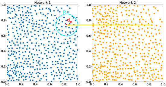
Figure 1.
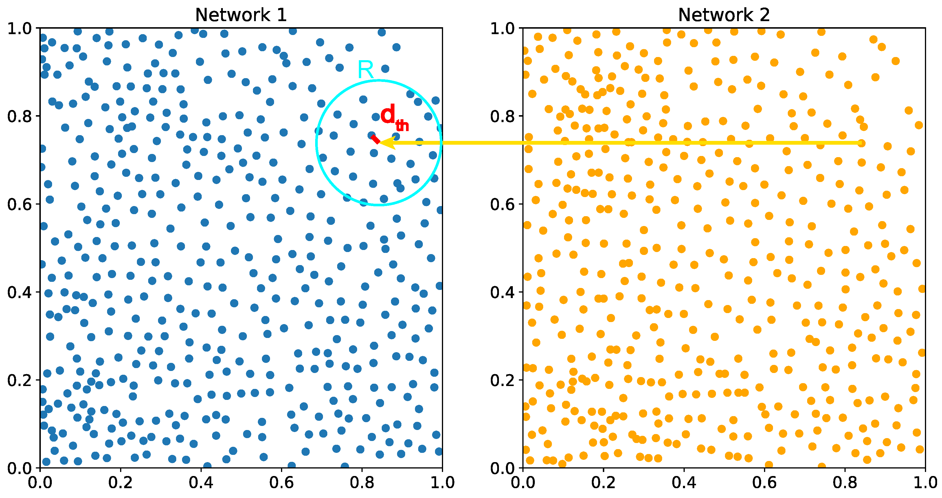
An illustration of the operating principle of the SOM. The two networks represent the particles of two consecutive images. Each neuron is input into the opposite network, and if a BMU is found within a threshold distance , all neurons within a radius R are activated, and their weights are updated accordingly. The blue dots represent the particles in network 1, while the orange dots correspond to particles in network 2. The activation radius R is shown in turquoise, and the threshold distance is visualized in red.
This entire procedure—alternating input from both networks—is repeated for a predefined number of iterations, after which the matching process is considered complete. With each iteration, the initially large radius r decreases linearly, until in the final iterations, only the weights of the BMU are adjusted, while neighboring neurons remain unaffected. This approach enables large-scale structural adaptations during early iterations and the fine-tuning of local matching accuracy in the final stages. Conversely, the adjustment factor increases over iterations by a factor , as described by
with .
At the end of the iterative process, the neurons in both networks have self-organized such that corresponding neurons are positioned topologically close to one another. The final matching is evaluated by comparing the distances between neurons in both networks. If two neurons are separated by less than a predefined threshold —measured by their Euclidean distance as defined in Equation (2)—they are considered a match, and the corresponding particles they represent are paired. If multiple candidate matches are identified, the closest one is selected.
Computational Optimization
The SOM matches particles by arranging representative neurons based on their mutual distances. Consequently, during the matching process, the Euclidean distance between all particle pairs must be computed. Since the SOM operates iteratively, this calculation is performed multiple times. As a result, the computational complexity increases exponentially with the number of particles and linearly with the number of iterations. This can lead to substantial computation times, which may limit the applicability of the SOM for real-time analysis.
To enhance performance, particle distances are computed only once at the beginning of each iteration. Neuron weight updates are then calculated and accumulated, with the final adjustments applied at the end of the iteration.
To address the challenge of high particle counts in large images, the image is divided into smaller sub-images with overlapping edges. The overlap should significantly exceed the typical particle displacement to ensure proper matching. Particles are matched within these smaller segments with considerably reduced computational effort, and the segments are merged upon completion. Special attention is required during merging to eliminate duplicate particles resulting from overlapping regions. If two duplicate particles are matched to different counterparts, the match with the smallest distance is retained.
With these improvements, the computation time for matching two consecutive 2048 × 2048 images containing over 17,000 particles was reduced from over four minutes to approximately five seconds by dividing the image into 16 smaller segments—without introducing matching errors at the segment boundaries.
2.2. Hyperparameter Optimization
The particle matching process described above operates without the need for prior initialization or training. The algorithm requires only the input data in the form of x and y coordinates of particles from two consecutive images, along with a set of predefined SOM hyperparameters: , , , , the number of iterations, and the initial and final radii and for the linear decrease. These hyperparameters are typically initialized with values that yield good overall performance. Based on previous SOM implementations [8,22,23,24], the typical parameter ranges are as follows: between 0.002 and 0.011, from 0.7 to 1, between 0.03 and 0.05, number of iterations between 5 and 100, from 60 to 40 and from 0.1 to 0.0001. The threshold distance should be larger than the average particle displacement between images. These hyperparameters directly affect the performance of the matching process. While these settings provide good results for simple and slow particle flows, careful initialization is essential to maintaining robust matching performance in high- flows. The influence of each parameter on the matching process is discussed below.
The initial radius may need to be adjusted when particle density varies. However, as long as it is large enough to encompass several neighboring neurons, its impact on performance remains limited. In contrast, the final radius and the minimum matching distance should remain small, regardless of particle density or displacement. This is because is intended to include only the BMU neuron and , as the matching criterion, strongly influences the risk of incorrect particle matches.
At higher particle displacements, other hyperparameters exert a more significant influence. For effective self-organization, the network must accommodate the displacement range, which depends on the values of , and , and the number of iterations. If any of these parameters are set too low, neurons may be unable to overcome large displacements, resulting in missed or incorrect matches. In cases where , this can lead to particle matches that falsely indicate movement in the opposite direction of the actual flow.
This phenomenon is observed when analyzing increasingly fast complex-plasma particle clouds using the SOM. As particle velocity increases while maintaining constant density, the matching performance deteriorates significantly, rendering reliable analysis infeasible. Trackpy [7], commonly used in complex-plasma experiments, also fails to accurately identify particle traces under these conditions, even when employing its adaptive linking feature. Therefore, the objective is to identify optimized hyperparameter regions that enable accurate particle tracking at high velocities using the SOM.
To achieve this, isotropic particle clouds are randomly generated at a fixed particle density of 0.002 , closely matching the actual complex-plasma densities observed in current experiments. An adjustable horizontal displacement is then applied to simulate particle motion. The cloud is constructed by continuously adding particles at random positions while maintaining a minimum distance between them until the target density is reached. To further align the synthetic data with experimental conditions, random noise is added in both the x and y directions.
Particles are displayed within a 512 × 512 pixel window, and 200 time steps of movement are generated. The SOM is initialized with various combinations of , and values, along with different iteration counts, before being applied to the synthetic dataset. After each run, the matching results are evaluated, and the matching performance is calculated as the percentage of correctly matched particles out of all possible matches. This procedure enables the systematic analysis of hyperparameter effects and the identification of optimal configurations.
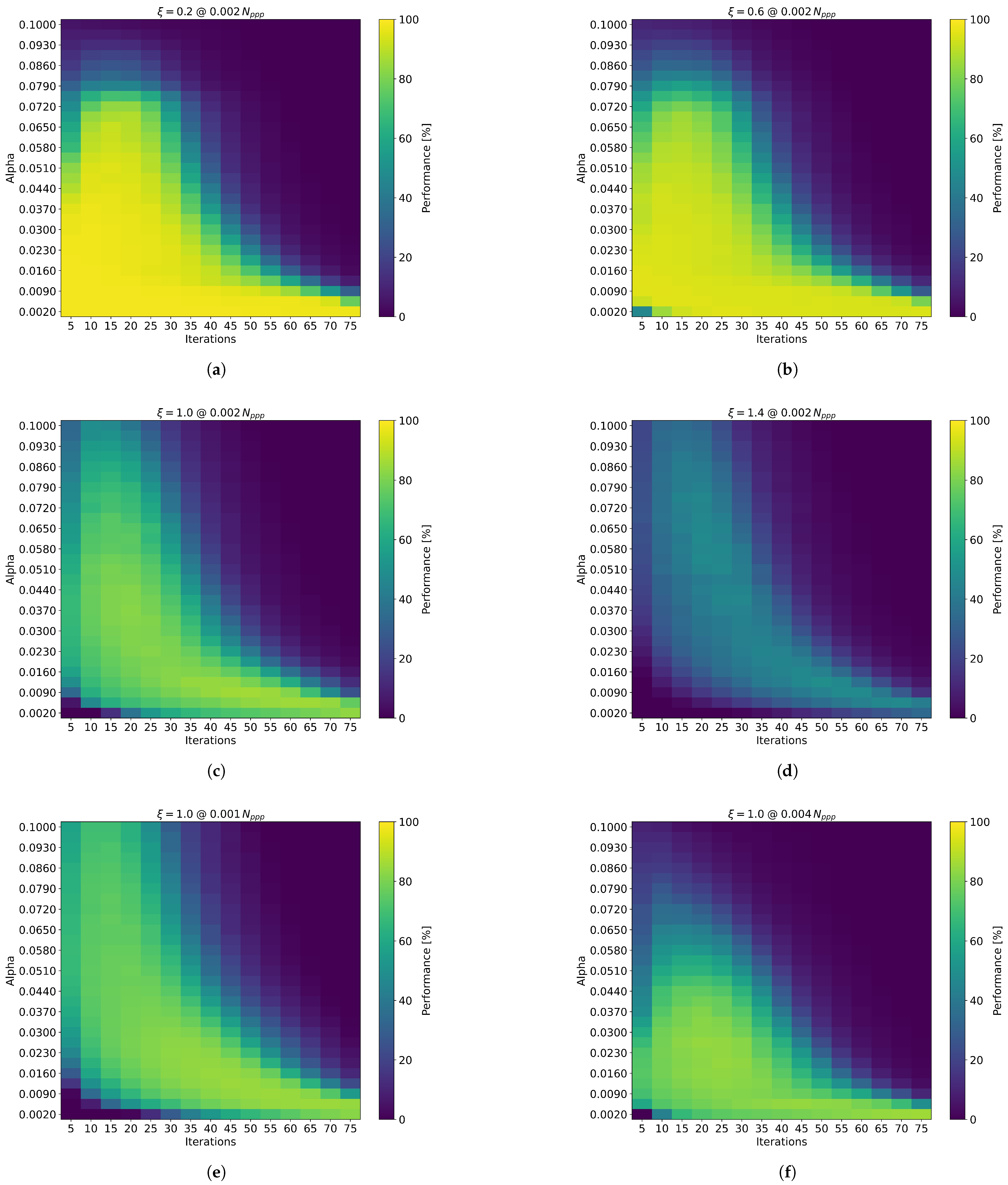
In our tests, the SOM consistently performed best with a value of 0.95 across all scenarios; therefore, this value was fixed for the sake of presentation. The threshold distance was automatically set to 1.3 times the particle displacement per time step in the artificial dataset. Consequently, the remaining parameters— and the number of iterations—were calibrated relative to the corresponding value of the synthetic data. Representative results are illustrated in Figure 2, and a comprehensive summary is provided in Table 1.
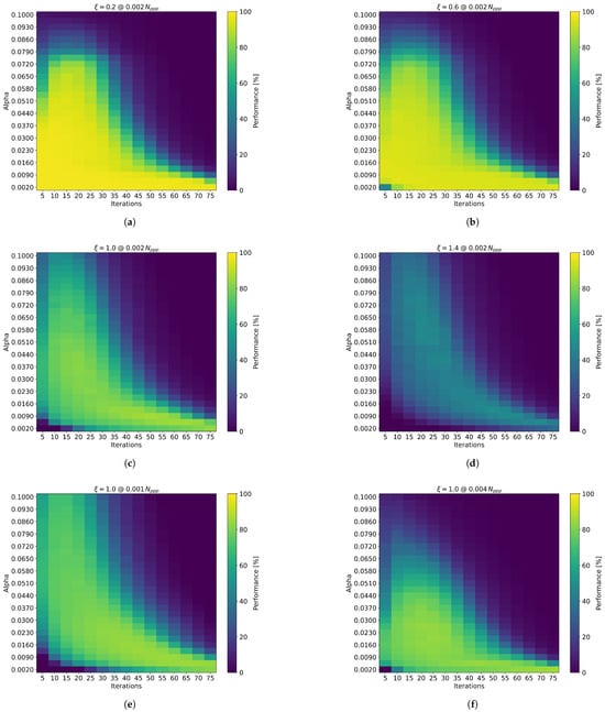
Figure 2.
Exemplary displays of particle matching results for varying and iteration settings across different values. (a) Results for , (b) , (c) and (d) . Subfigures (e) and (f) both depict at particle densities of 0.001 and 0.004 , respectively. The color scale represents the percentage of correctly matched particles relative to all possible matches.

Table 1.
Optimal and iteration values for flows with different values that maximize particle matching performance. The corresponding best performance is reported as the percentage of correctly matched particles relative to all possible matches.
It is expected that for flows with the same value but different particle densities—and thus different particle displacements over time steps—the SOM will yield similar overall matching performance. However, the optimal value and number of iterations may vary depending on the specific displacement characteristics. This behavior is analyzed for flows with a value of 1.0 at different particle densities.
3. Results
The results clearly demonstrate that the and iteration settings play a critical role in particle matching performance. As expected, higher values require a combination of increased and/or a greater number of iterations to achieve accurate particle matching. It is evident that for higher values, increasing the number of iterations is generally more effective than increasing . Figure 2 further illustrates that the range of hyperparameter values yielding good matching performance narrows as increases. Therefore, for high flow speeds, the careful tuning of SOM hyperparameters is essential. The optimal and iteration values are summarized in Table 1.
Notably, the matching performance drops significantly at values of 1.0 and above, and even more so beyond , where the SOM identifies only about half of the possible particle matches. Remarkably, these results are achieved solely by adjusting the hyperparameters to the flow conditions, without requiring prior knowledge of the flow direction. Nevertheless, to ensure optimal accuracy for subsequent data analysis, robust outlier detection and error assessment remain crucial—particularly in this challenging regime.
Direct comparisons with other SOM implementations are limited due to differences in particle flow characteristics and the scarcity of detailed documentation in published studies. However, our results qualitatively align with the hyperparameter configurations reported by Ji et al. [23], who used 100 iterations to achieve convergence in wind-blown sand flow analysis, emphasizing the necessity of extended training cycles in highly dynamic environments. In contrast, Hoseini et al. [24] observed convergence in just 12 iterations when tracking rod-like particles in dispersed two-phase flows, even under high- conditions (). Our empirical observations suggest that increasing the iteration count while lowering can yield measurable improvements in performance, supporting the idea of extended optimization even after apparent convergence. These findings underscore the importance of context-specific hyperparameter tuning in SOM-based PTV, especially when balancing computational efficiency and matching accuracy in complex flow regimes.
The hyperparameter optimization was conducted for a fixed particle density of 0.002 . Particle flows with the same value but varying particle densities and corresponding displacements are illustrated in Figure 2c,e,f. As a result, the SOM exhibits comparable performance for flows with higher densities and lower displacements, as well as for those with lower densities and higher displacements, provided that the value remains constant. Consequently, SOM matching performance primarily depends on the flow’s value. However, variations in particle density influence the optimal hyperparameter settings—particularly the value. In this study, the hyperparameters were fully calibrated for the specific case of 0.002 . For applications involving different particle densities, either the value must be scaled accordingly, or the particle coordinates should be rescaled to maintain consistent matching behavior.
To support broader applicability, an automated hyperparameter calibration feature has been integrated into the SOM implementation. This functionality streamlines the tuning process for key parameters, particularly and the number of iterations, by adapting them to the characteristics of the particle flow. The calibration involves matching particles between the first two images in the dataset while systematically varying the hyperparameters within predefined ranges. For each configuration, the algorithm evaluates performance by calculating the percentage of correctly matched particles relative to the total number of matchable particles. This quantitative assessment enables the identification of the hyperparameter combination that yields maximum matching accuracy. By automating this calibration step, the SOM becomes more adaptable to diverse flow conditions and significantly reduces the need for manual fine-tuning, thereby enhancing its robustness and practical utility across a wide range of applications.
In conclusion, the particle matching performance of the SOM in low- flows is very good, requiring only minor adjustments to the hyperparameters. In high- flows, characterized by elevated particle densities and velocities, careful hyperparameter tuning becomes essential to achieving accurate matching and reliable results. However, due to the increased likelihood of errors under such conditions, robust performance additionally depends on the availability of sufficient data and the implementation of effective outlier filtering techniques.
3.1. Validation on Experimental Complex-Plasma Data
To further validate the effectiveness of our hyperparameter-optimized SOM, we applied it to experimental complex-plasma data obtained from recent PK-4 experiments conducted on the International Space Station and during parabolic flights. The experimental data featured fast-moving plasma particle clouds with values reaching up to 1.34. The optimized SOM successfully tracked particles in these flows, demonstrating both robustness and accuracy under real-world conditions.
Due to the fact that the experimental data are unlabeled, it is not possible to provide an exact quantitative assessment of accuracy or matching performance. However, detailed results and a comprehensive analysis of this application have been published by Wimmer et al. [2]. These findings confirm that the proposed hyperparameter tuning framework enables reliable PTV even in highly challenging experimental scenarios.
3.2. Comparison Overview
With optimal hyperparameter settings for the SOM, a direct comparison to the conventional method Trackpy becomes feasible. This comparison is carried out using artificially generated complex particle flow data under various conditions to evaluate and verify matching performance. Artificial data are used to enable a controlled, qualitative comparison with definitive ground truth while maintaining similarity to real complex-plasma datasets.
In addition, a widely accepted method for validating particle tracking performance involves the use of VSJ PIV standard images [25], which is also employed here to provide a comprehensive assessment of particle matching performance.
3.2.1. Evaluation on Synthetic Data
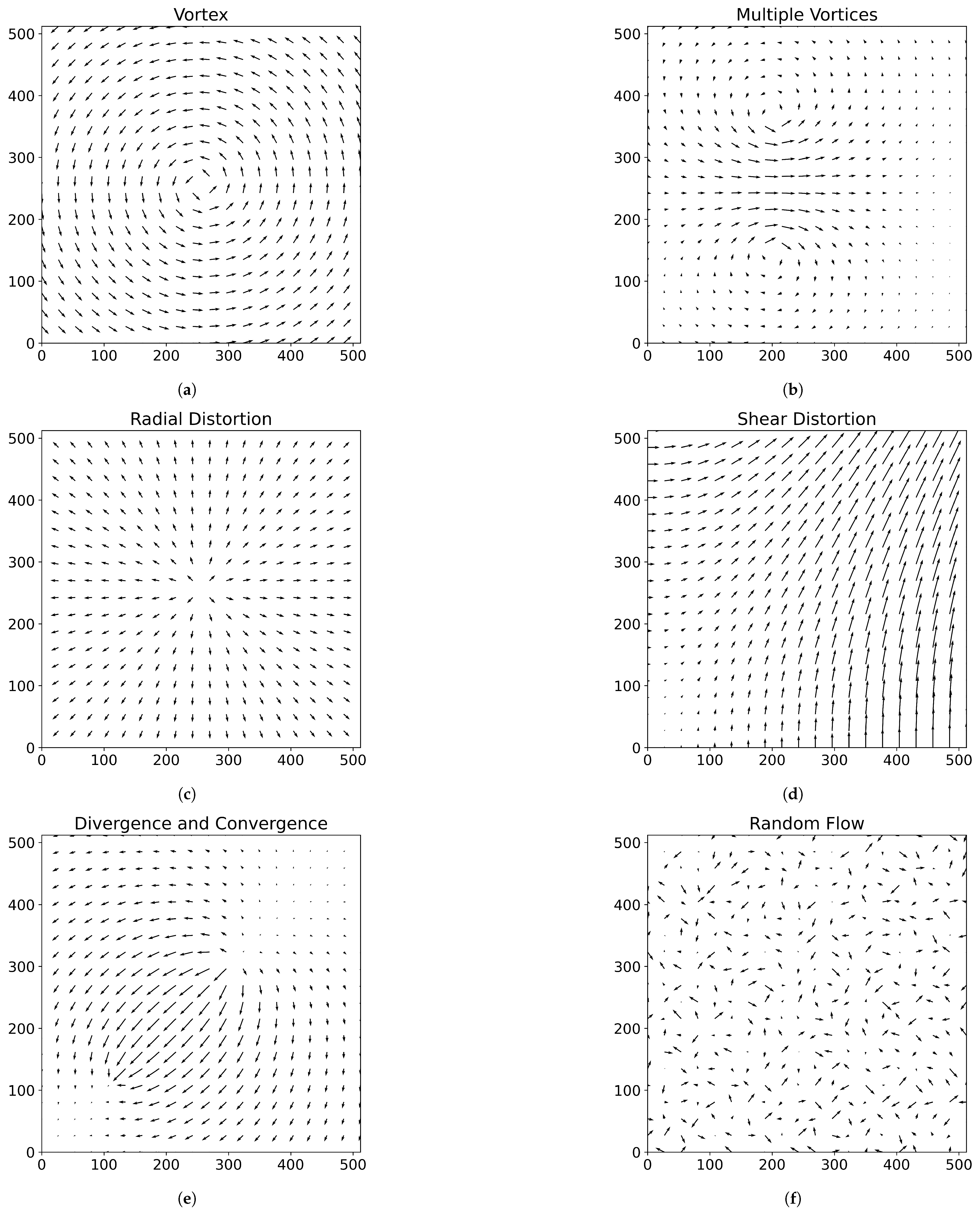
Similar to Section 2.2, isotropic particle distributions are generated and various flow fields are applied. These flow fields range from simple laminar flows to more complex scenarios, including multiple vortex flows, radial distortion, shear flows, divergent and convergent flows and random turbulent motion—designed to represent a wide range of possible flow situations. The schematics of the synthetic flow types are presented in Figure 3.
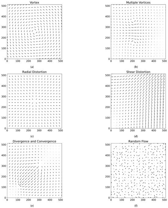
Figure 3.
Vector flow fields used to generate synthetic particle flow data for comparing the matching performance of the SOM and Trackpy algorithms. The length of each arrow indicates the flow speed of the corresponding particles. Subfigures depict the following flow types: (a) single vortex flow, (b) multiple vortex flow, (c) radial distortion flow, (d) shear distortion flow, (e) divergent and convergent flow and (f) random flow.
The laminar flow field is used to evaluate the impact of increasing particle displacement over time steps. The two vortex flow fields introduce the challenge of directional changes, one in a uniform and the other in a more irregular manner. The radial distortion flow tests the ability to detect non-coherent, omnidirectional motion. Shear, divergent and convergent flows introduce particle motion with strongly varying speeds and local densities. Finally, the random flow field simulates fully inconsistent and chaotic motion.
These synthetic flows are applied at varying intensities, and the matching performance of both algorithms is assessed. The corresponding value is calculated based on the mean particle displacement per time step and the mean particle density, which is fixed at 0.002 to closely replicate real complex-plasma data. For particle matching, the Trackpy algorithm is used with adaptive linking enabled. A comprehensive comparison of results is provided in Table 2, where matching performance is reported as the ratio of correctly matched particle pairs to all possible pairs.
Table 2.
Matching performance of SOM and Trackpy algorithms for different flow types and values. Performance is defined as the percentage of correctly matched particles relative to all possible particle matches.
It is clearly evident that the SOM consistently outperforms Trackpy under high- flow conditions. Beginning with the laminar flow case, the SOM maintains strong performance even at high particle displacements over successive time steps, whereas Trackpy’s performance rapidly declines below 50% for values exceeding 0.6. Similar trends are observed in the vortex flow scenarios: while Trackpy delivers acceptable results only at very low displacements, the SOM maintains high accuracy. In the single vortex case, the SOM’s performance remains nearly constant up to , with only a slight drop being observed for multiple vortices. In contrast, Trackpy becomes ineffective as particle velocities increase.
Comparable results are found for the radial distortion and divergent/convergent flows, where the SOM significantly outperforms Trackpy across the tested values. An exception is observed in the shear flow, where Trackpy shows marginally better performance relative to other cases. This can be attributed to the presence of very slow-moving particles in the lower region of the image, which remain easily matchable. Since the value is calculated based on the mean particle speed, the impact of these nearly stationary particles skews the apparent difficulty of the scenario.
The only case where Trackpy consistently outperforms the SOM is the random flow field. In this highly chaotic regime, both algorithms experience a marked decline in performance, but Trackpy maintains a slight advantage. This is likely due to the rapidly and unpredictably changing flow directions, which present a particular challenge for the SOM. While both methods struggle under these conditions, the SOM exhibits a more pronounced drop in accuracy.
3.2.2. Evaluation on VSJ PIV Images
To further quantify the particle matching performance of the SOM and Trackpy algorithms, both methods were applied to VSJ PIV standard image #301 [25]. A similar evaluation has previously been conducted for a SOM implementation [22], although in that case, particle positions were identified by using dynamic binary thresholding prior to matching. This approach detected only a subset of the particles, thereby significantly reducing the effective particle density in the image. In contrast, our analysis considers all known particle positions.
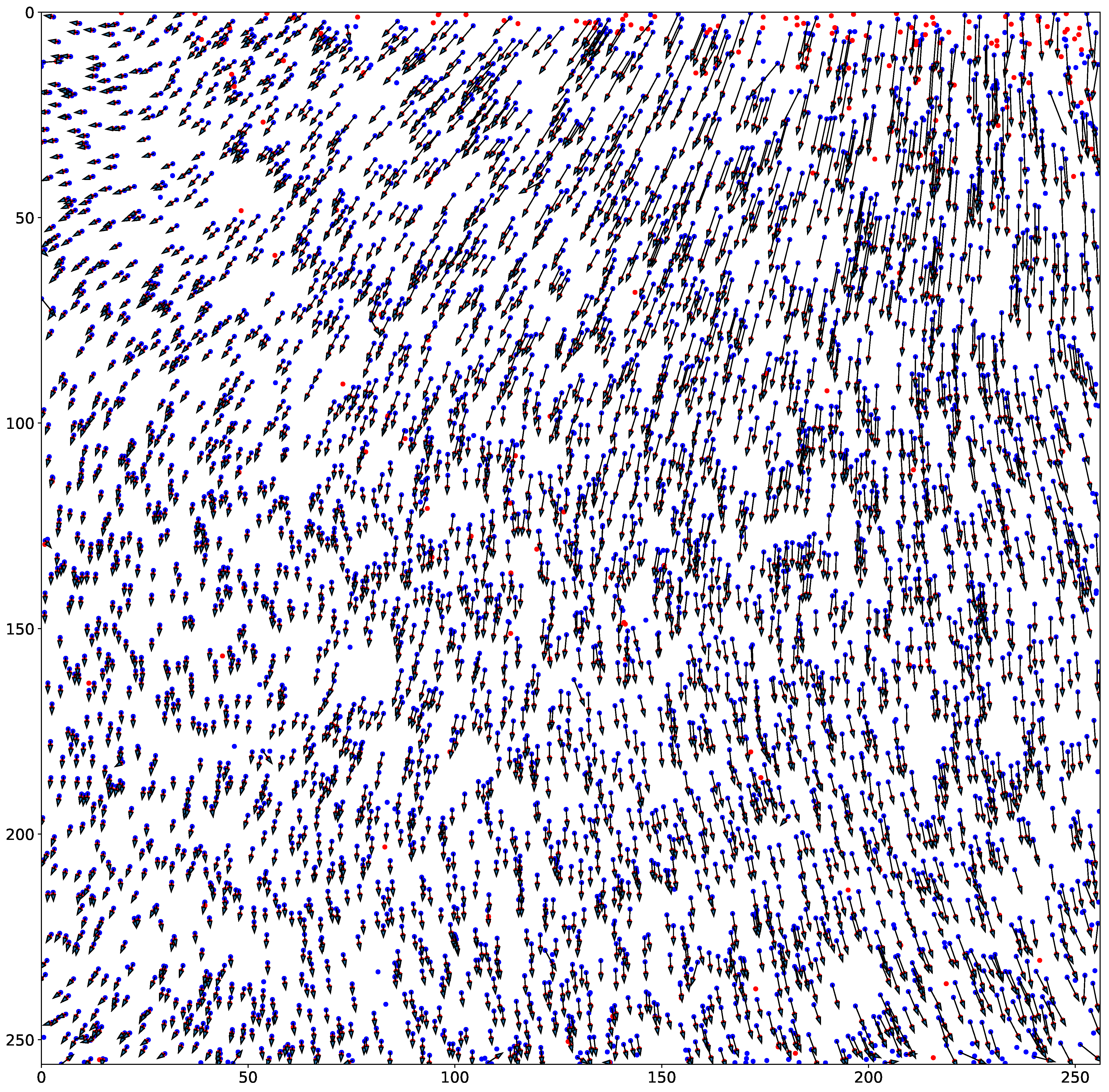
Among the 4042 matchable particles in the #301 image, the SOM successfully identified 3959 matches, of which 3829 were correct. This corresponds to a matching yield of 97.95% and a reliability of 96.72%. The test was performed by using an value of 0.002 and 15 iterations, which yielded the best results for this dataset. The hyperparameters were optimized by using the same method described in Section 2.2, though lower values were optimal in this case due to the higher particle density of the image, measured at 0.061 . The matching performance across different hyperparameter settings is visualized in the heatmap in Figure 4, and the matched particle pairs are illustrated in Figure 5.
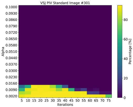
Figure 4.
Particle matching results for varying and iteration settings on the VSJ PIV standard image #301 [25]. The color scale represents the percentage of correctly matched particles relative to all possible particle matches.
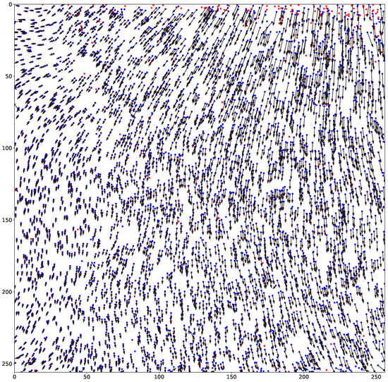
Figure 5.
Visualization of all particles in the first two VSJ PIV standard images, #301 [25]. Particles from the first image are shown in blue, and particles from the second image are shown in red. Arrows indicate the particle matches identified by the SOM.
In comparison, Trackpy produced only 3337 matches, of which just 1160 were correct. This corresponds to a matching yield of 28.7% and a match reliability of 34.76%.
The SOM demonstrates impressive performance across a wide range of flow speeds, particle densities and values, underscoring its versatility in particle matching tasks. These results highlight the SOM’s potential not only for complex-plasma experiments but also for a broad range of other applications. Furthermore, the SOM significantly outperforms Trackpy, as evidenced by its substantially higher matching yield and reliability in the evaluation using the VSJ PIV standard image.
3.3. Outlier Detection Using LSTM Network
When it comes to detecting outliers, multiple approaches are available, ranging from simple velocity and/or directional filters [26] to continuity-based evaluations [27] and more advanced methods such as fuzzy logic, which enables more nuanced decision making for individual particles [28]. While these algorithms can yield excellent results, they generally require calibration to a specific dataset. When filter ranges and fuzzy logic rules are appropriately configured, outlier filtering is straightforward. However, in chaotic or poorly characterized flows, these approaches may fall short.
To address this limitation, we introduce a novel outlier detection method based on a Long Short-Term Memory (LSTM) neural network, which analyzes particle trajectories to identify and remove defective traces.
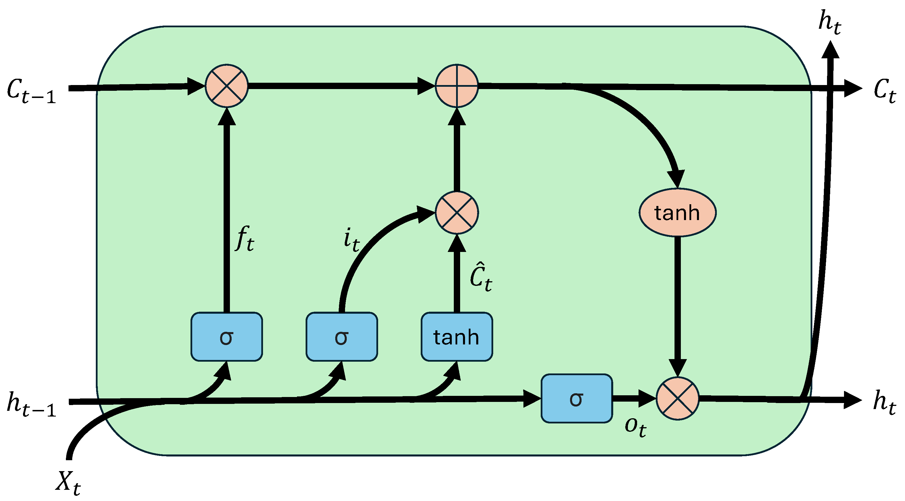
The LSTM network is a type of recurrent neural network (RNN) characterized by a memory cell that retains past information, making them particularly effective for sequential data analysis. In contrast to traditional neural networks, where the output depends solely on the current input and fixed weights, LSTM maintains both a cell state and a hidden state , which—together with the current input —are used to compute the next states and output.
An LSTM cell comprises three gates: the forget gate , the input gate and the output gate . The forget gate determines which information from the previous cell state should be discarded; the input gate controls how much new information is stored; and the output gate governs the contribution of the cell state to the final output. These operations utilize nonlinear activation functions, primarily the sigmoid function , which produces gating values between 0 and 1, and the tanh function, which maps values to the range for smooth, bounded transformations.
A schematic of the LSTM cell is presented in Figure 6. The ability of LSTMs to model temporal dependencies is particularly advantageous for analyzing sequential datasets such as particle trajectories. Their memory structure allows them to extract meaningful patterns across sequences of varying length and complexity, making them well suited for robust outlier detection in particle tracking applications.

Figure 6.
Schematic of LSTM cell. The previous cell state , hidden state and current input are processed through the forget gate , input gate and output gate , as indicated by the arrows. The blue boxes represent the sigmoid and tanh activation functions, while the red circles denote the corresponding arithmetic operations. The updated cell state and the output of the LSTM cell are shown on the right.
LSTM networks are particularly well suited for outlier detection in sequential data due to their ability to model long-range temporal dependencies. Previous studies have demonstrated their effectiveness in identifying anomalies across various domains. For example, Chen et al. [29] employed LSTM autoencoders to detect anomalies in particle accelerator systems, achieving high accuracy in identifying orbit lock anomalies. Similarly, Ergen and Kozat [30] proposed an LSTM-based framework that integrates One-Class Support Vector Machines (OC-SVMs) and Support Vector Data Description (SVDD) for unsupervised anomaly detection in variable-length sequences. Saha et al. [31] introduced a Quantile LSTM for detecting anomalies in industrial time-series data, while Park et al. [32] utilized an ensemble of LSTM autoencoders to identify outliers in indoor air quality monitoring.
Beyond anomaly detection, LSTMs have also been applied to predict and filter trajectory-based motion patterns. Hug et al. [33] developed a Long Short-Term Memory with Minimum Description Length (LSTM-MDL) model for pedestrian path prediction, demonstrating the LSTM’s capability to filter anomalous movement patterns and optimize trajectory representations in sequential data.
Inspired by these developments, we propose an LSTM-based method to detect incorrect particle traces in PTV. Our approach analyzes sequential particle displacements and directional changes to identify and filter trajectories that significantly deviate from expected motion patterns. Unlike prior applications focused on accelerator monitoring, industrial fault detection or pedestrian tracking, our method is specifically designed for tracking particle motion in complex-plasma flows, representing a novel adaptation of LSTM networks within this context.
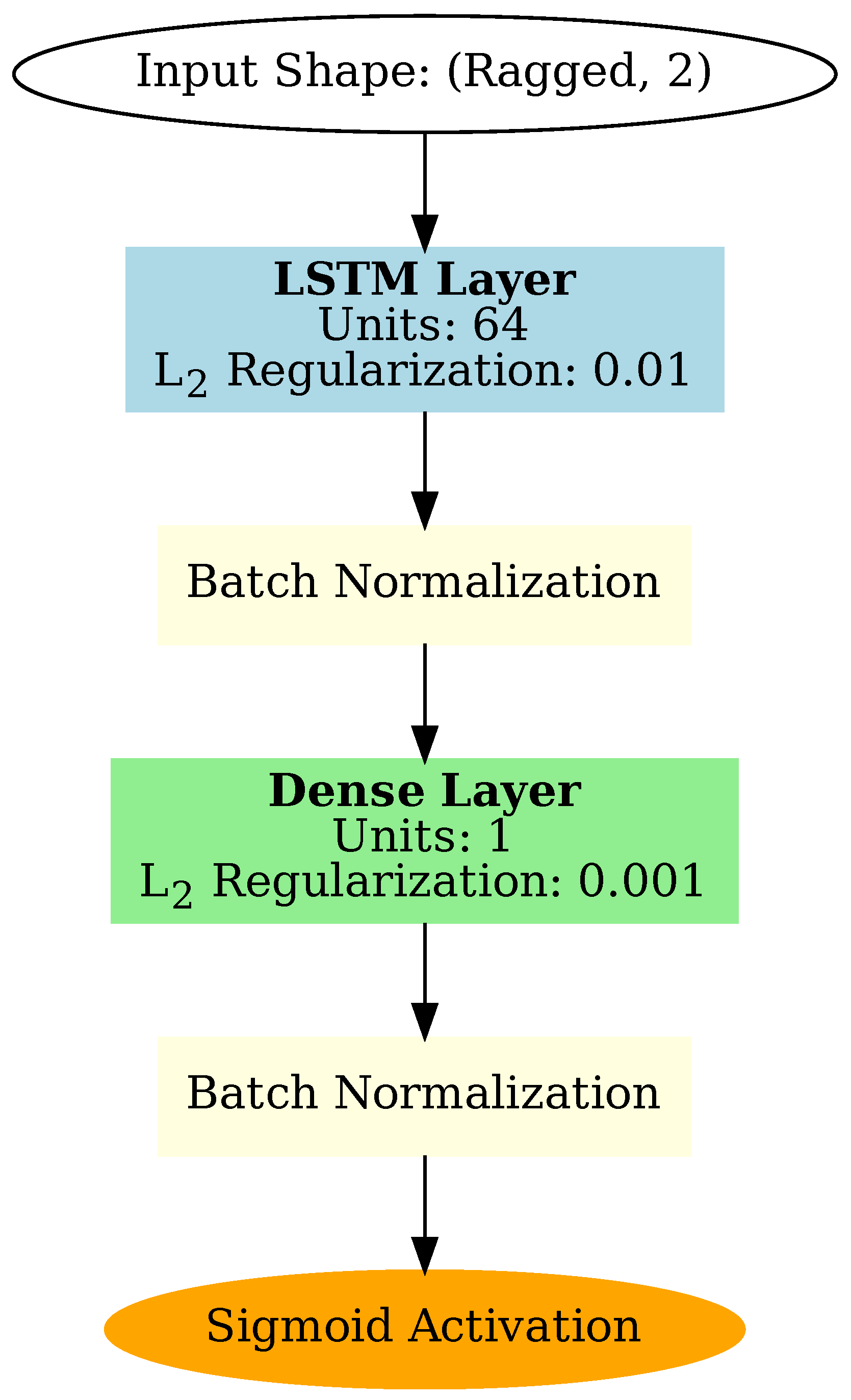
An LSTM neural network is constructed, beginning with a ragged input layer that accepts sequences of variable lengths, each containing two features. This is followed by an LSTM layer with 64 units and L2 regularization (0.01) to reduce the risk of overfitting. A batch normalization layer is applied after the LSTM layer to stabilize and accelerate training. The output layer consists of a dense layer with a single neuron, also employing L2 regularization (0.001), followed by another batch normalization layer and a sigmoid activation function to produce the final output. A schematic of the network architecture is shown in Figure 7. The sigmoid output determines whether the input particle trace is classified as correct (output = 1) or faulty (output = 0).
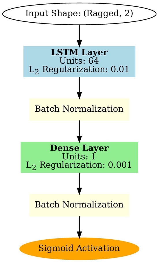
Figure 7.
A schematic of the LSTM network used for filtering defective particle traces. The input layer accepts sequences of variable length, enabling the analysis of particle traces with differing durations. The output is passed through a sigmoid activation function to classify each trace as valid or faulty.
Synthetic particle trace data are used for training. Following the approach described in Section 2.2, isotropic particle clouds are randomly generated at various densities, and flow fields are applied to produce labeled particle positions over successive time steps. A combination of laminar and vortex flow fields with varying directions and intensities is used to simulate diverse motion patterns. These flows are also superimposed with random fluctuations to enhance realism. Correct particle traces are extracted from the labeled dataset. To simulate faulty traces, half of the correct trajectories are modified by replacing one or two matched particles with incorrect neighbors at random positions, thereby imitating common tracking errors. The resulting traces are labeled accordingly, with correct traces assigned a label of 1 and incorrect traces assigned a label of 0.
Prior to training, each particle trace—comprising a sequence of particle coordinates—is transformed into a sequence of features representing the distance and angle between successive matched particles. These features are then converted into relative values by expressing each distance and angle in relation to those of the preceding step. This results in a two-dimensional vector sequence representing relative distances and angles.
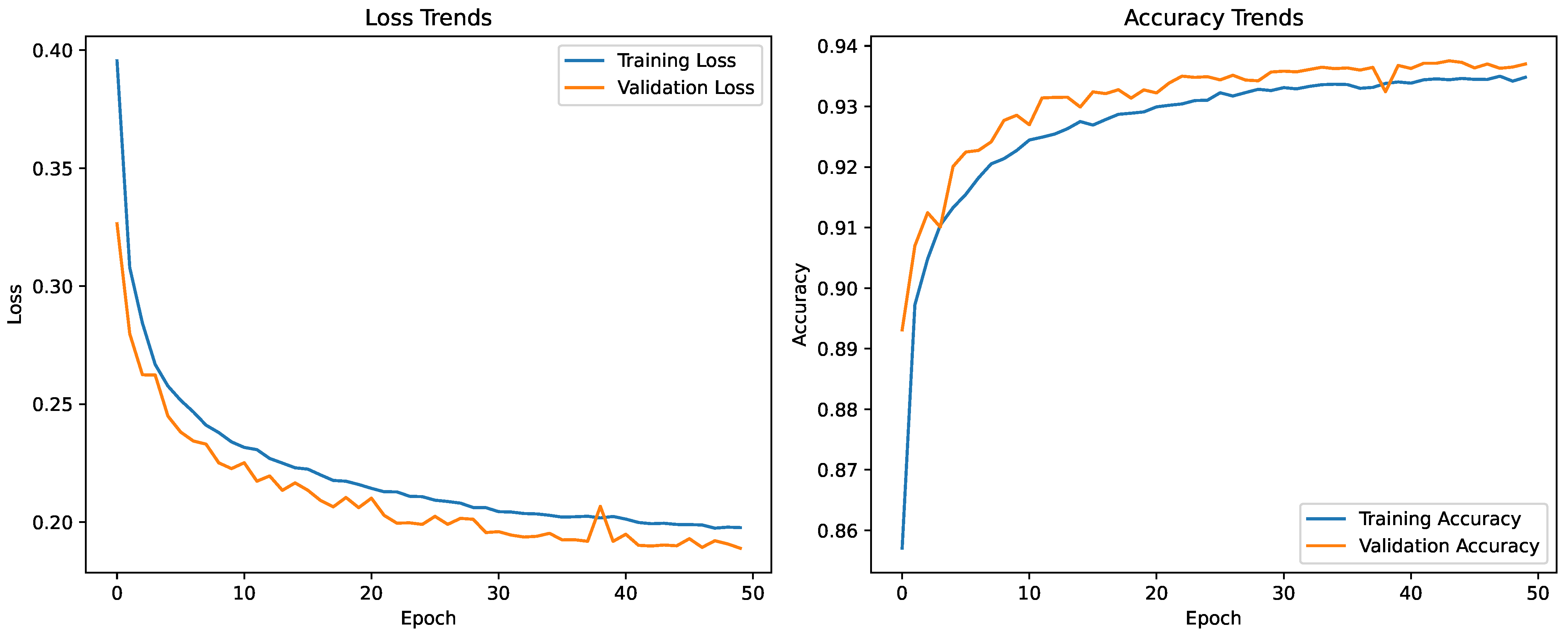
A total of 170,000 traces are generated for training, equally divided between correct and incorrect cases. The dataset is split, with 20% used for validation during training. Approximately 67% of the traces are derived from laminar flow data and 33% from vortex flow data. The model is trained by using the Adam optimizer [34] with an initial learning rate of 0.0001. The learning rate is reduced by a factor of 0.5 after three consecutive epochs without improvement, with a final minimum learning rate of 0.0000125. Binary cross-entropy (BCE) is used as the loss function to quantify the discrepancy between predicted probabilities and true labels. Early stopping is employed to prevent overfitting, terminating the training process after five consecutive epochs without improvement. Training concludes after 48 epochs, achieving a final accuracy of 93.5%.
Figure 8 shows the training history, including loss and accuracy over all epochs, to illustrate model performance. After training, the model achieves a recall of 97.6% and a precision of 90.4%, indicating that it successfully detects nearly all outliers, though it may occasionally misclassify correct traces as outliers.
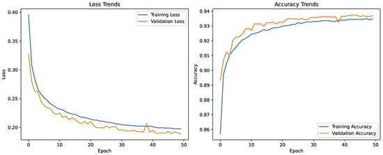
Figure 8.
Training and validation loss and accuracy trends during the training of the LSTM-based outlier detection model.
To validate the performance of the LSTM-based outlier detection method, we conducted a comparative evaluation against three additional outlier detection algorithms applied to various particle flow scenarios. The first algorithm was a simple threshold-based approach, which filters particles exhibiting abrupt changes in velocity magnitude or angular displacement. The second method employed a continuity filter that evaluates the temporal consistency of individual particle trajectories. The third was a fuzzy logic-based algorithm that assigns an outlier probability to each particle match based on predefined rules and parameter ranges; this probability determines whether a match is classified as correct or incorrect. All four algorithms, including the LSTM method, were tested on three distinct particle flow datasets to assess their performance under different conditions.
The first two datasets consisted of synthetic particle flows designed to simulate laminar and vortex flow patterns. In both cases, particles were randomly distributed across the domain with a minimum inter-particle distance enforced to ensure isotropic spacing. A laminar flow field was applied to the first dataset, while the second incorporated a vortex velocity field. To introduce additional complexity and realism, random noise was added to the particle motion in both datasets, simulating deviations from idealized flow and increasing the difficulty of outlier detection.
The third dataset consisted of VSJ PIV standard image set #301 [25], a widely used benchmark for validating particle image velocimetry (PIV) methods. To evaluate algorithm robustness, artificial outliers were introduced into all three datasets at contamination levels of 5%, 10% and 15%. These outliers were created by randomly selecting particle trajectories and replacing segments with sections from neighboring trajectories—effectively mimicking realistic tracking errors without relying on overly simplified anomalies such as large, easily detectable jumps.
Prior to outlier detection, all datasets were preprocessed by using the SOM for particle trajectory matching. To simulate challenging conditions, SOM parameters were left unoptimized, resulting in an initial outlier density of approximately 50%. This setup provides a rigorous testing environment for the algorithms.
In the evaluation, a particle trace is classified as incorrect if it contains at least one outlier, regardless of whether the algorithm analyzes complete trajectories or individual particles. For algorithms that flag individual particle-level outliers, the corresponding full trace is marked as incorrect. This standardized evaluation protocol ensures a consistent and fair comparison across all algorithmic approaches.
The performance of each outlier detection algorithm depends heavily on both the characteristics of the data and the specific parameter settings of the algorithms. In this study, algorithm parameters were coarsely tuned to each particle flow scenario but were not subjected to detailed optimization for maximum performance. This approach was chosen to ensure a fair comparison with the LSTM-based method, which benefits from end-to-end learning and does not require explicit parameter tuning. While this lack of optimization leaves room for potential improvements in the results of the traditional algorithms, the chosen configurations still provide meaningful benchmarks for evaluating the LSTM’s performance.
The datasets used in this study pose substantial challenges for outlier detection, given their high noise levels, realistic particle densities and carefully constructed outliers that are not trivially identifiable. Despite these complexities, the LSTM-based algorithm demonstrated strong and consistent performance without the need for manual parameter adjustment. In contrast, traditional methods relied on heuristic thresholds and rules that required manual tuning for each dataset.
The full results of the comparative analysis are presented in Table 3. Two key performance metrics are reported: the total number of detected outliers and the percentage of correctly identified outliers among those detected. These metrics offer insights into the sensitivity of each method and the reliability (precision) of outlier detection.
Table 3.
Detection rates and reliability of outlier detection algorithms in laminar, vortex and VSJ PIV flows across varying outlier contamination levels.
The performance comparison of the four outlier detection methods across different flow regimes and outlier density levels reveals several key insights. The LSTM-based approach consistently demonstrated high reliability—exceeding 74%—in detecting outliers without requiring parameter tuning, particularly excelling in complex scenarios such as vortex flows. In contrast, the threshold-based method exhibited variable performance, with a high rate of false positives at low contamination levels but improved reliability under extreme outlier densities. Notably, the LSTM network’s ability to recognize temporal patterns enabled it to outperform other methods in vortex flows, achieving perfect reliability at a 15% outlier contamination level. However, at very high outlier levels (around 50%), the LSTM network’s detection rate declined significantly, indicating limitations in handling extreme contamination. This performance crossover suggests that LSTM is particularly well suited for moderate contamination levels in complex flows, while traditional methods may be more effective in severely corrupted datasets.
Although traditional outlier detection algorithms may achieve improved results when carefully calibrated to specific particle flow conditions, the LSTM network’s performance is remarkable—especially considering its applicability to previously unseen flow fields. Furthermore, when the underlying flow characteristics are known, the training data can be augmented with synthetic traces tailored to that flow type, enhancing model performance in targeted applications. In this study, the first 30 frames of the VSJ PIV standard image sequence were isolated and used as training data, while the remaining images were reserved for evaluation. After 20 additional epochs of retraining on these data, the LSTM detected 16.34% of outliers with a reliability of 83.57%, demonstrating substantial performance gains through targeted fine-tuning.
It is important to note that due to the sequential nature of the LSTM model, outlier detection is not feasible when only two consecutive images are available. A minimum of three or more time steps is required to construct analyzable particle traces. Beyond outlier detection, this type of neural network holds potential for broader applications. For instance, it could be trained to classify particle trace characteristics, such as distinguishing between turbulent and laminar flows, provided that appropriate labeled training data are available. In this way, particle traces could be analyzed for dynamic properties previously inaccessible through traditional methods.
In combination with the SOM, the LSTM outlier detection model expands the particle tracking framework, offering robust and adaptive analysis capabilities for complex and unknown flow conditions.
4. Discussion
In conclusion, this study presents the comprehensive hyperparameter optimization of the SOM, enabling its effective application to high- flow scenarios—particularly relevant for fast complex-plasma experiments. While traditional methods such as Trackpy perform well under lower-density and simpler-flow conditions, they encounter substantial limitations in high-density, high-velocity and rotational flow environments typical of complex plasmas. This work demonstrates that the SOM algorithm, with its adaptability and minimal initialization requirements, provides a more reliable and robust approach to accurately tracking particles across a wide range of flow conditions.
A central factor contributing to the SOM’s success is the fine-tuning of hyperparameters to optimize particle matching performance across various values, representing different flow intensities and particle displacements. By evaluating SOM performance on artificially generated particle flows with controlled velocity profiles, this study identified optimal ranges for parameters such as and the number of iterations. Such optimization significantly improved matching accuracy, including in regimes with . The enhanced SOM configuration facilitates its application in high-speed complex-plasma experiments, where traditional algorithms often suffer from high error rates. An integrated automated hyperparameter optimization function further supports efficient deployment in unknown flow scenarios.
Beyond SOM calibration, this study introduces a novel outlier detection method using an LSTM neural network to refine particle trajectory accuracy. The LSTM’s ability to model temporal dependencies allowed it to achieve an accuracy of 93.5% in identifying and filtering incorrect particle matches. This significantly reduced false positives and improved the overall reliability of the particle tracking process. Particularly in flows with unpredictable directional changes, this data-driven approach enables a more automated and less manually intensive analysis pipeline. The combination of SOM for particle matching and LSTM for outlier detection thus provides a unified and powerful framework for PTV in complex-plasma research.
Comparative analyses against Trackpy further confirmed the superior performance of the SOM-based framework. The SOM consistently outperformed Trackpy across a diverse set of synthetic flow patterns—including vortices, radial distortions, shear flows and divergent/convergent flows—maintaining high reliability even in regimes with significant rotational, velocity and density gradients. While Trackpy remained effective for simpler laminar flows, its accuracy declined rapidly with the increase in and trajectory complexity. The SOM’s adaptability, combined with computational enhancements such as image segmentation and parallelized weight updates, not only preserved accuracy but also reduced processing time substantially, supporting the feasibility of real-time applications and automated workflows in plasma diagnostics.
Overall, this research study establishes the SOM, augmented by LSTM-based error detection, as a versatile and high-performance solution for PTV in dynamic and complex environments. The insights into optimal hyperparameter ranges and computational efficiency render this approach highly suitable for complex-plasma studies and transferable to other fields involving dense particle flows, such as atmospheric physics and fluid dynamics. Future work may further extend this framework by integrating additional machine learning models to capture specific flow features. Moreover, the LSTM-based network could be adapted for advanced particle trace analysis, such as turbulence classification or flow regime identification, unlocking new capabilities for understanding complex fluid behaviors.
Author Contributions
Conceptualization, M.K. and N.D.; methodology, M.K.; software, M.K.; validation, M.K.; formal analysis, M.K.; investigation, M.K. and N.D; resources, M.K.; data curation, M.K., N.D. and L.W.; writing—original draft preparation, M.K.; writing—review and editing, M.K., N.D., L.W., M.H.T. and M.S.; visualization, M.K.; supervision, M.K.; project administration, M.H.T. and M.S.; funding acquisition, M.H.T. and M.S. All authors have read and agreed to the published version of the manuscript.
Funding
This research study was funded by the German Federal Ministry of Economic Affairs and Climate Action under grant number 50WK2270B.
Institutional Review Board Statement
Not applicable.
Data Availability Statement
The original contributions presented in this study are included in the article. Further inquiries can be directed to the corresponding author.
Acknowledgments
This work was supported by the German Aerospace Agency (DLR). We thank the research group of Markus H. Thoma at Justus Liebig University Giessen for providing the data used in this study and the German Aerospace Society for providing powerful PCs in accordance with the funding decision, which facilitated the studies.
Conflicts of Interest
The funders had no role in the design of the study; in the collection, analyses, or interpretation of data; in the writing of the manuscript; or in the decision to publish the results.
Abbreviations
The following abbreviations are used in this manuscript:
| PTV | particle tracking velocimetry |
| SOM | Self-Organizing Map |
| LSTM | Long Short-Term Memory |
| PK-4 | Plasmakristallexperiment 4 |
| BMU | best-matching unit |
| BCE | binary cross-entropy |
| OC-SVM | One-Class Support Vector Machine |
| SVDD | Support Vector Data Description |
| LSTM-MDL | Long Short-Term Memory with Minimum Description Length |
References
- Dabiri, D.; Pecora, C. Particle tracking techniques. In Particle Tracking Velocimetry; IOP Publishing: Bristol, UK, 2019; pp. 5-1–5-60. [Google Scholar] [CrossRef]
- Wimmer, L.; Dormagen, N.; Klein, M.; Kretschmer, M.; Lipaev, A.M.; Schwarz, M.; Usachev, A.D.; Petrov, O.F.; Zobnin, A.; Thoma, M. Impact of particle charge and electrorheology-effects on dust-acoustic waves in low pressure complex plasma under microgravity. New J. Phys. 2025, 27, 033001. [Google Scholar] [CrossRef]
- Schwabe, M.; Zhdanov, S.; Räth, C. Turbulence in an auto-oscillating complex plasma. IEEE Trans. Plasma Sci. 2017, 46, 684–687. [Google Scholar] [CrossRef]
- Schmitz, A.S.; Schulz, I.; Kretschmer, M.; Thoma, M.H. Dust cloud convections in inhomogeneously heated plasmas in microgravity. Microgravity Sci. Technol. 2023, 35, 13. [Google Scholar] [CrossRef]
- Thomas, H.M.; Morfill, G.E. Melting dynamics of a plasma crystal. Nature 1996, 379, 806–809. [Google Scholar] [CrossRef]
- Pustylnik, M.; Fink, M.; Nosenko, V.; Antonova, T.; Hagl, T.; Thomas, H.; Zobnin, A.; Lipaev, A.; Usachev, A.; Molotkov, V.; et al. Plasmakristall-4: New complex (dusty) plasma laboratory on board the International Space Station. Rev. Sci. Instrum. 2016, 87, 093505. [Google Scholar] [CrossRef]
- Allan, D.B.; Caswell, T.; Keim, N.C.; van der Wel, C.M.; Verweij, R.W. Soft-Matter/Trackpy, v0.6.1; Zenodo: Geneva, Switzerland, 2023. [Google Scholar] [CrossRef]
- Klein, M.; Dormagen, N.; Schmitz, A.S.; Thoma, M.H.; Schwarz, M. Machine Learning Approach for Particle Matching, Tracing and Velocimetry with Self-Organizing Map: Application to Complex Plasmas. In Proceedings of the 2023 International Conference on Machine Learning and Applications (ICMLA), Jacksonville, FL, USA, 15–17 December 2023; pp. 839–844. [Google Scholar]
- Hassan, Y.; Canaan, R. Full-field bubbly flow velocity measurements using a multiframe particle tracking technique. Exp. Fluids 1991, 12, 49–60. [Google Scholar] [CrossRef]
- Malik, N.; Dracos, T.; Papantoniou, D. Particle tracking velocimetry in three-dimensional flows: Part II: Particle tracking. Exp. Fluids 1993, 15, 279–294. [Google Scholar] [CrossRef]
- Ouellette, N.T.; Xu, H.; Bodenschatz, E. A quantitative study of three-dimensional Lagrangian particle tracking algorithms. Exp. Fluids 2006, 40, 301–313. [Google Scholar] [CrossRef]
- Yamamoto, F.; Uemura, T.; Tian, Z.H.; Ohmi, K. Three-Dimensional PTV Based on Binary Cross-Correlation Method: Algorithm of Particle Identification. JSME Int. J. Ser. Fluids Therm. Eng. 1993, 36, 279–284. [Google Scholar] [CrossRef]
- Hassan, Y.; Blanchat, T.; Seeley, C., Jr. PIV flow visualisation using particle tracking techniques. Meas. Sci. Technol. 1992, 3, 633. [Google Scholar] [CrossRef]
- Saga, T.; Kobayashi, T.; Segawa, S.; Hu, H. Development and evaluation of an improved correlation based PTV method. J. Vis. 2001, 4, 29–37. [Google Scholar] [CrossRef]
- Jambunathan, K.; Ju, X.; Dobbins, B.; Ashforth-Frost, S. An improved cross correlation technique for particle image velocimetry. Meas. Sci. Technol. 1995, 6, 507. [Google Scholar] [CrossRef]
- Wu, Q.X.; Pairman, D. A relaxation labeling technique for computing sea surface velocities from sea surface temperature. IEEE Trans. Geosci. Remote Sens. 1995, 33, 216–220. [Google Scholar] [CrossRef]
- Baek, S.; Lee, S. A new two-frame particle tracking algorithm using match probability. Exp. Fluids 1996, 22, 23–32. [Google Scholar] [CrossRef]
- Ohmi, K.; Li, H.Y. Particle-tracking velocimetry with new algorithms. Meas. Sci. Technol. 2000, 11, 603. [Google Scholar] [CrossRef]
- Brevis, W.; Niño, Y.; Jirka, G. Integrating cross-correlation and relaxation algorithms for particle tracking velocimetry. Exp. Fluids 2011, 50, 135–147. [Google Scholar] [CrossRef]
- Grant, I.; Pan, X. An investigation of the performance of multi layer, neural networks applied to the analysis of PIV images. Exp. Fluids 1995, 19, 159–166. [Google Scholar] [CrossRef]
- Labonté, G. A new neural network for particle-tracking velocimetry. Exp. Fluids 1999, 26, 340–346. [Google Scholar] [CrossRef]
- Ohmi, K. SOM-based particle matching algorithm for 3D particle tracking velocimetry. Appl. Math. Comput. 2008, 205, 890–898. [Google Scholar] [CrossRef]
- Ji, L.; Yang, F.; Guan, M. The Application of SOM Network to Particle Tracking Velocimetry in a Wind-Blown Sand Flow. In Proceedings of the 2015 2nd International Conference on Information Science and Control Engineering, Shanghai, China, 24–26 April 2015; pp. 493–496. [Google Scholar]
- Abbasi Hoseini, A.; Zavareh, Z.; Lundell, F.; Anderson, H.I. Rod-like particles matching algorithm based on SOM neural network in dispersed two-phase flow measurements. Exp. Fluids 2014, 55, 1705. [Google Scholar] [CrossRef]
- Okamoto, K.; Nishio, S.; Saga, T.; Kobayashi, T. Standard images for particle-image velocimetry. Meas. Sci. Technol. 2000, 11, 685. [Google Scholar] [CrossRef]
- Sun, J.; Yates, D.; Winterbone, D. Measurement of the flow field in a diesel engine combustion chamber after combustion by cross-correlation of high-speed photographs. Exp. Fluids 1996, 20, 335–345. [Google Scholar] [CrossRef]
- Song, X.; Yamamoto, F.; Iguchi, M.; Murai, Y. A new tracking algorithm of PIV and removal of spurious vectors using Delaunay tessellation. Exp. Fluids 1999, 26, 371–380. [Google Scholar] [CrossRef]
- Sapkota, A.; Ohmi, K. Error detection and performance analysis scheme for particle tracking velocimetry results using fuzzy logic. Int. J. Innov. Comput. Inf. Control 2009, 5, 4927–4934. [Google Scholar]
- Chen, Z.; Lu, W.; Bhong, R.; Hu, Y.; Freeman, B.; Carpenter, A. Anomaly Detection of Particle Orbit in Accelerator using LSTM Deep Learning Technology. arXiv 2024, arXiv:2401.15543. [Google Scholar]
- Ergen, T.; Kozat, S.S. Unsupervised anomaly detection with LSTM neural networks. IEEE Trans. Neural Netw. Learn. Syst. 2019, 31, 3127–3141. [Google Scholar] [CrossRef]
- Saha, S.; Sarkar, J.; Dhavala, S.; Sarkar, S.; Mota, P. Quantile LSTM: A Robust LSTM for Anomaly Detection In Time Series Data. arXiv 2023, arXiv:2302.08712. [Google Scholar]
- Park, J.; Seo, Y.; Cho, J. Unsupervised outlier detection for time-series data of indoor air quality using LSTM autoencoder with ensemble method. J. Big Data 2023, 10, 66. [Google Scholar] [CrossRef]
- Hug, R.; Becker, S.; Hübner, W.; Arens, M. Particle-based pedestrian path prediction using LSTM-MDL models. In Proceedings of the 2018 21st International Conference on Intelligent Transportation Systems (ITSC), Gold Coast, QLD, Australia, 18–21 November 2018; pp. 2684–2691. [Google Scholar]
- Kingma, D.P. Adam: A method for stochastic optimization. arXiv 2014, arXiv:1412.6980. [Google Scholar]

Disclaimer/Publisher’s Note: The statements, opinions and data contained in all publications are solely those of the individual author(s) and contributor(s) and not of MDPI and/or the editor(s). MDPI and/or the editor(s) disclaim responsibility for any injury to people or property resulting from any ideas, methods, instructions or products referred to in the content. |
© 2025 by the authors. Licensee MDPI, Basel, Switzerland. This article is an open access article distributed under the terms and conditions of the Creative Commons Attribution (CC BY) license (https://creativecommons.org/licenses/by/4.0/).