Abstract
This article advances the research on the intelligent monitoring and control of helicopter turboshaft engines in onboard conditions. The proposed neural network system for anomaly prediction functions as a module within the helicopter turboshaft engine monitoring and control expert system. A SARIMAX-based preprocessor model was developed to determine autocorrelation and partial autocorrelation in training data, accounting for dynamic changes and external factors, achieving a prediction accuracy of up to 97.9%. A modified LSTM-based predictor model with Dropout and Dense layers predicted sensor data, with a tested error margin of 0.218% for predicting the TV3-117 aircraft engine gas temperature values before the compressor turbine during one minute of helicopter flight. A reconstructor model restored missing time series values and replaced outliers with synthetic values, achieving up to 98.73% accuracy. An anomaly detector model using the concept of dissonance successfully identified two anomalies: a sensor malfunction and a sharp temperature drop within two minutes of sensor activity, with type I and II errors below 1.12 and 1.01% and a detection time under 1.611 s. The system’s AUC-ROC value of 0.818 confirms its strong ability to differentiate between normal and anomalous data, ensuring reliable and accurate anomaly detection. The limitations involve the dependency on the quality of data from onboard sensors, affected by malfunctions or noise, with the LSTM network’s accuracy (up to 97.9%) varying with helicopter conditions, and the model’s high computational demand potentially limiting real-time use in resource-constrained environments.
1. Introduction
1.1. Relevance of the Research
In the context of rapid technological development and the increasing amounts of data collected by sensor systems [1], there is a need to develop methods for detecting anomalous data. Predicting anomalous data in sensor systems is vital in critical areas such as aviation [2,3], medicine [4,5], energy [6], and industrial production [7,8]. Sensor systems collect and analyze large amounts of data in real time, enabling the control and monitoring of various processes and conditions [9]. Due to equipment wear, interference, or calibration errors, data anomalies can occur, indicating potential failures or malfunctions that lead to economic losses or safety threats [10]. Therefore, developing methods for effectively predicting and detecting anomalous data is crucial for ensuring the reliability and safety of sensor systems.
Modern approaches to anomaly prediction use machine learning methods [11,12] and artificial intelligence [13,14] to identify the hidden patterns and trends in large amounts of data. These methods adapt to changing conditions and provide timely warnings of potential issues, allowing for preventive measures and risk minimization. This article’s scientific relevance stems from the need to improve algorithms’ accuracy and speed, necessitating research on model optimization and data-processing enhancement. In the context of the increasing digitization and reliance on automated systems, anomaly prediction is becoming a key element in maintaining their stable and efficient operation.
1.2. State of the Art
In recent years, researchers have actively applied machine learning and artificial intelligence methods, such as neural networks, clustering, and outlier detection techniques. Machine learning [11,12] and artificial intelligence [13,14] play a key role in predicting anomalous data. Deep learning algorithms, including recurrent [15,16] and convolutional neural networks [17,18], have been proven effective in processing time series data from sensors. Studies [15,16,17,18] show that combining different neural network architectures can enhance anomaly prediction accuracy and reliability. For example, using autoencoders to identify hidden patterns in data ensures high accuracy in detecting anomalies in complex systems, such as aviation and industrial installations [19,20].
Alongside machine learning methods, statistical methods [21,22] and clustering techniques [22,23] are widely used for predicting anomalous data. Statistical approaches, such as probability density estimation and principal component analysis, identify deviations from normal data behavior. Clustering methods, like k-means and hierarchical clustering, group data and detect anomalies based on differences between clusters. These methods are often combined with machine learning to enhance prediction quality.
Research also focuses on the practical integration of anomaly prediction methods into industrial applications [24]. Implementing such systems significantly improves equipment monitoring and diagnostics, preventing failures and reducing downtime. For example, in aviation, anomaly prediction systems help detect potential faults in engines and other critical components, ensuring higher levels of safety and reliability [25]. Similarly, in the energy sector, these systems optimize control processes and reduce the risk of emergencies [26].
The application of neural networks for predicting anomalous data in sensor systems is scientifically justified due to their ability to efficiently process large amounts of data and identify complex, nonlinear dependencies [27,28] that are difficult to detect using traditional methods [29,30]. Their capability to train from historical data enables adaptive prediction [31], which is crucial in changing, dynamic systems, such as aviation and industrial applications. Moreover, the ability to automatically extract features from data makes neural networks a powerful tool for anomaly detection, minimizing the need for manual tuning and data preprocessing [32]. This enhances anomaly detection accuracy and reliability, which is critical for ensuring the safety and resilience of sensor systems.
1.3. Main Attributes of the Research
The object of the research is the sensor data.
The subject of the research includes the neural network system for predicting anomalous data in sensor systems.
The research aim is to develop a neural network system for predicting anomalous data in sensor systems, which will provide enhanced accuracy and speed in detecting data deviations, allowing for timely responses to potential failures and malfunctions.
To achieve this aim, the following scientific and practical tasks were solved:
- Development of the proposed neural network system for predicting anomalous data in sensor systems.
- Development of the preprocessor model.
- Development of the predictor model.
- Development of the reconstructor model.
- Development of the anomaly detector model.
- Conducting a computational experiment involving the simulation of predictive anomalies for a sensor in a helicopter turboshaft engine (TE).
The main contribution of this research lies in developing a neural network system for predicting anomalous data in sensor systems, which will, in turn, enhance the reliability and safety of critical systems, minimize economic losses by preventing emergencies, and optimize maintenance and operation processes. The developed system will be capable of adapting to changing conditions and system dynamics, providing more effective real-time control and monitoring.
2. Materials and Methods
2.1. Development of the Proposed Neural Network System for Predicting Anomalous Data in Sensor Systems
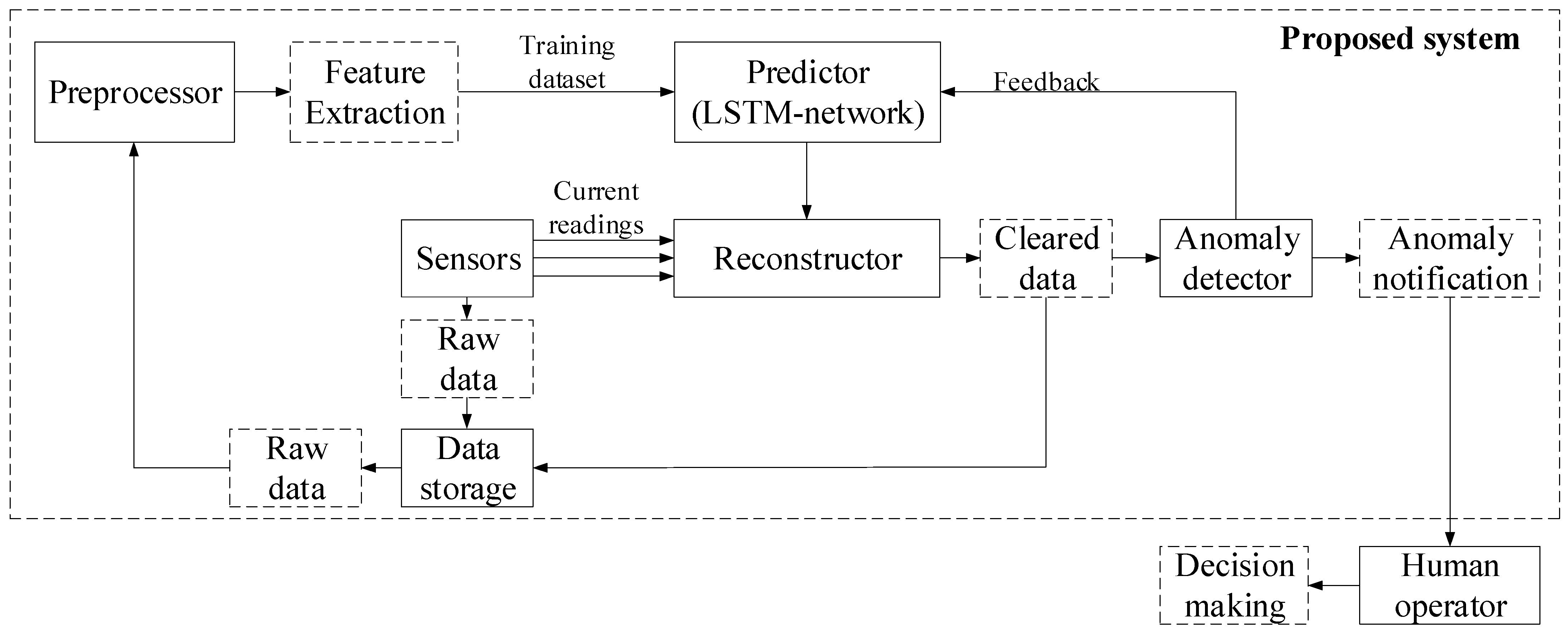
The block diagram of the proposed neural network system for predicting anomalous data in sensor systems (hereinafter referred to as the “system”) is shown in Figure 1. The system is created for each sensor of the sensor system under research and includes a preprocessor, predictor, reconstructor, and anomaly detector.
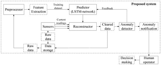
Figure 1.
Block diagram of the proposed neural network system for predicting anomalous data in sensor systems.
The preprocessor prepares sensor data for subsequent processing. The predictor uses a neural network to predict the next sensor value based on historical data. The reconstructor checks if the current value is an outlier and replaces it with the predicted value from the predictor if necessary. The anomaly detector identifies anomalous sequences in the data to alert the operator. The working cycle of the sensor data cleaning module is as follows. The preprocessor operates at a frequency set by the operator, extracting raw data from storage and forming a training dataset for the predictor’s neural network. The predictor runs according to the data acquisition frequency, predicting the current value. If the sensor returns an empty value, it is replaced with the predicted one. Otherwise, the reconstructor classifies the value as either an outlier or normal. If an anomalous value is recognized, it is replaced with the predicted one. The system then transmits this value for storage. At the end of the cycle, the anomaly detector determines if an anomalous sequence is ending and notifies the operator if necessary.
When the predicting system detects anomalous data, it performs a series of actions to ensure accurate reporting and system integrity. Upon identifying an anomaly, the system initially replaces the anomalous data with the predicted value from the neural network. Following this replacement, the anomaly detector assesses whether the anomalous sequence is concluding. If the sequence is deemed significant, the system generates a notification for the operator, providing a detailed analysis of the detected anomalies. This analysis includes information on the anomalies and the nature of the potential impacts on the sensor system, enabling the operator to make informed decisions regarding further actions or adjustments. Thus, the system not only corrects the data but also actively informs the operator about potential issues, enhancing overall system reliability and response capability.
2.2. Development of the Preprocessor Model
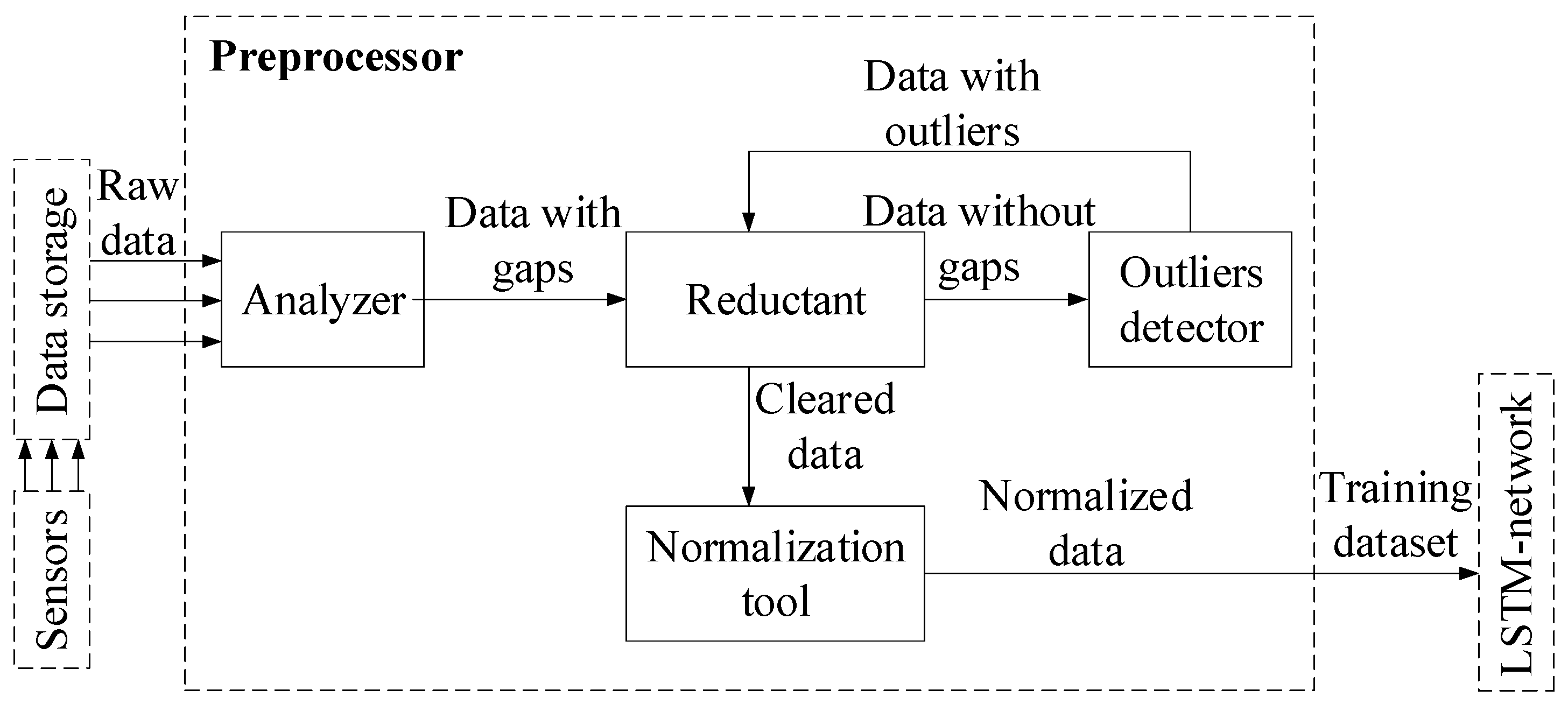
The preprocessor (Figure 2) prepares the training dataset for the neural network in the predictor subsystem and consists of the following components: an analyzer, restorer, outlier detector, and normalizer. The analyzer extracts sensor data from storage and converts it into a format suitable for further processing. The restorer then replaces missing values with synthetic ones. The outlier detector identifies anomalous points and replaces them with NULL. The processed data passes through the restorer again for outlier replacement. The normalizer forms normalized subsequences, which become the training dataset for the neural network.

Figure 2.
Block diagram of the preprocessor model.
The restorer uses the SARIMAX model to predict missing values and replace them with synthetic ones [33,34]. The SARIMAX model is defined by the equation:
where c is a constant, φ1, …, φp are the autoregressive coefficients, θ1, …, θq are the moving average coefficients, εt is the white noise, and Xt are the exogenous regressors. If ti = NULL, then
where is the predicted value obtained using the SARIMAX model. To check stationarity, the Dickey–Fuller and KPSS tests are used [35,36]. If the series is not stationary, transformations such as logarithms are applied to prepare the data for analysis.
The analyzer retrieves the time series T from the data store, where T = (t1, t2, …, tm), and each value ti belongs to the real numbers ℝ set or is empty (equal to NULL), that is
The normalizer then creates a training dataset consisting of “readings sequence” and “predicted value” pairs. The first element of a pair is the fixed-length sensor readings normalized subsequence, and the second element is a single normalized sensor reading following this subsequence. The normalizer transforms the time series into a set of normalized subsequences using min–max normalization. The sequence Ti,n of the time series T with length n is defined as
Ti,n = (ti, …, ti+n−1), 1 ≤ i ≤ m − n + 1.
Using min–max normalization, for a subsequence Ti,n, its normalized version is calculated as
where
where tmin and tmax are the minimum and maximum values in Ti,n.
For a normalized subsequence , the element is considered as its predicted value. The training sample is formed from pairs (subsequence, predicted value):
The subsequence length n (n << m) is the Cleanup Module parameter and is calculated as
where fsensor is the sensor frequency and horizon is the historical horizon (the time interval length in the past) used by the predictor and selected by the human operator.
n = fsensor · horizon,
2.3. Development of the Predictor Model
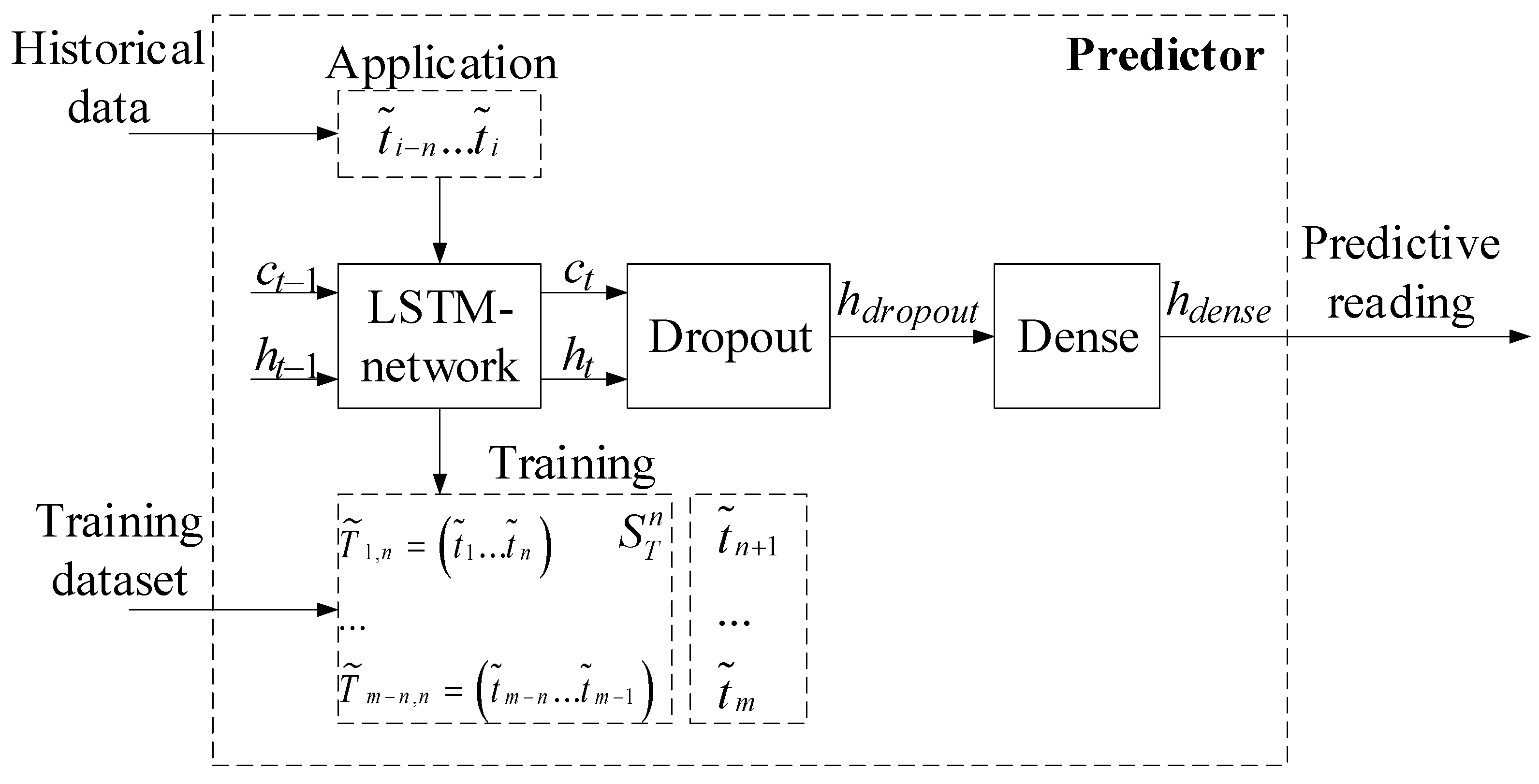
The predictor is a recurrent neural network (RNN) with a long short-term memory (LSTM) layer [37,38] (Figure 3). The RNN training is carried out on the dataset prepared by the preprocessor. During use, the neural network takes a subsequence of actual sensor values preceding the current value as input and outputs a predicted value.
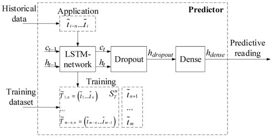
Figure 3.
Block diagram of the predictor model.
The LSTM layer consists of identical LSTM blocks (Figure 4), whose number matches the subsequence length n defined during preprocessing. These blocks collectively form a hidden state vector h, with its length set by the system operator. A Dropout layer randomly deactivates a specified neuron fraction in vector h to prevent overfitting, typically deactivating 20%, though this parameter can be adjusted by the operator. The Dense layer applies the modified (special) rectified linear unit (ReLU) activation function (Appendix A) to transform the data and obtain the predicted value ii+1.
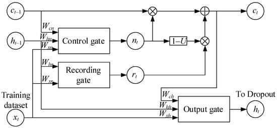
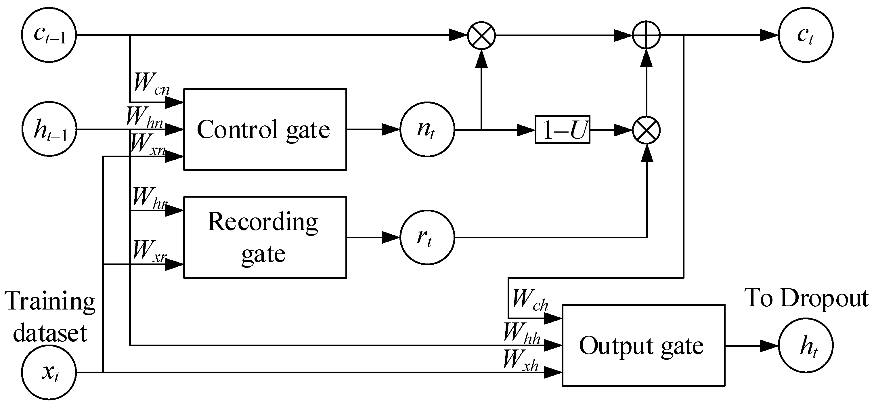
Figure 4.
Diagram of the variable memory LSTM network [37].
Each LSTM block comprises a block state and several filter layers. The block state is a vector carrying information from previous time steps and propagates through the entire chain of LSTM blocks. An LSTM block contains three types of filters (“gates”), an input gate, a forget gate, and an output gate, which regulate the data amount to be saved, forgotten, and output, respectively.
Figure 4 illustrates the following notations: the “Control gate” is a control unit with a sigmoidal activation function; the “Recording gate” is a recording unit with a tangential activation function; the “Output gate” is an output unit with a sigmoidal activation function; ct−1 is the memory tensor at the previous time step; ct is the memory tensor at the current time step; ht−1 is the network output tensor at the previous time step; ht is the network output tensor at the current time step; xt is the input tensor at the current time step; nt is the tensor at the control unit output; rt is the tensor at the recording unit output; and Wcn, Whn, Wxn, Whr, Wxr, Wch, Whh, and Wxh are the weight coefficients connecting inputs to units.
The LSTM mechanism addresses the vanishing gradient problem by regulating the flow of new information into the state vector ct, as well as the network’s output state ht, and updating its state ct. The vector filters are determined by the following expressions:
where σ is the sigmoid function; x is the input sequence; h is the network cell hidden state vector; and Ui, Uf, Uo, Ug, Wi, Wf, Wo, Wg are the network filter weight matrices for the training sequence element indices i, f, o, g, t.
Based on the network filter values, its internal state (internal memory) and hidden state vectors are determined as follows:
where ct represents the network cell state vector, ht denotes the hidden state vector, and “∘” indicates element-wise multiplication.
In the Dropout layer, certain elements of the activation vector are randomly set to zero to prevent overfitting. For an input activation vector h of size t and a mask vector m, where mask elements are either 0 or 1, the Dropout is expressed as
where “⊙” denotes element-wise multiplication, and m is the mask vector created randomly with probability p (the deactivated neuron proportion):
where p is the probability that the element will be deactivated, and is the scaling factor for maintaining the activation level during training.
After applying Dropout during training, the output vector hdropout is scaled by to preserve the expected output activation:
The Dense layer (or fully connected layer) transforms the input data through a linear combination followed by an activation function. An input activation vector hdropout of size n is transformed into an output activation vector hdense of size m using a weight matrix W and a bias b. The linear transformation is expressed as follows:
where W is an m × n weight matrix, b is a displacement vector of size m, and z is an intermediate output vector of size m.
z = W · hdropout + b,
The modified (special) ReLU activation function is applied to the intermediate output z to obtain the final output vector hdense:
that is
and
hdense = ReLU(z),
hdense = ReLU(z1), ReLU(z2), …, ReLU(zm),
ReLU(zi) = max(0, zi).
Thus, for each element zi in vector z, if zi > 0, it remains unchanged, and if zi ≤ 0, then it is replaced by 0.
2.4. Development of the Reconstructor Model
The reconstructor receives the current sensor reading and checks whether it is significantly different from the denormalized synthetic value received from the predictor. If the difference is significant, the real value is replaced with a synthetic one, which is then stored in the database. The reconstructor implementation is based on the prediction error probability distribution use [39]. In accordance with this approach, the difference threshold ε > 0 between the real sensor reading ti+1 and the predicted synthetic sensor value is determined. The prediction error at step i + 1 is defined as
The difference threshold ϵ is calculated as
where μ is the predicting error average value calculated from historical data; δ is the predicting error standard deviation calculated from historical data; and k is a parameter determined by the system operator (for example, k = 3).
ϵ = μ + k · δ,
If the prediction error ei+1 exceeds the threshold ϵ, then the current reading ti+1 is considered an outlier, that is
If ei+1 ≥ ϵ, then ti+1 is an outlier.
If ti+1 is an outlier, then it is replaced with the predicted value , which is then stored in the data store, that is
2.5. Development of the Anomaly Detector Model
The anomaly detector assesses whether a sensor reading subsequence, ending with the current value, constitutes an anomaly. If it is identified as such, the detector generates a notification for the monitoring sensor system operator. The specified subsequence length is defined by values corresponding to significant time intervals, which are calculated based on the sensor’s sampling frequency. The implementation of the anomaly detector uses the concept of dissonance [40]. Dissonance, unlike most anomaly detection algorithms, requires only one intuitive parameter, the anomalous subsequence length, and is formally defined as follows: Let T be the sensor reading time series; is the set of all possible subsequences of length n in T; Ti,n is the subsequence of length n starting at position i; D is the subsequence under investigation for anomalies; MD is the set of all subsequences that are not trivial matches with D; and k is the parameter defined by the system operator indicating the significance level. The Euclidean distance between the two subsequences Ti,n and Tj,n is defined as
where Tj,n is the subsequence of length n starting at position j.
Subsequences Ti,n and Tj,n are not trivial matches if there exists a subsequence (where i < p < j) such that
ED(Ti,n, Tj,n) < ED(Ti,n, Tp,n).
Subsequence is called dissonance if
where MC is the set of all subsequences that are not trivial matches to C.
Subsequence is called the most significant k-th dissonance in T if
where is the set of the k-th closest subsequence that is not a trivial match to D.
Let ti+1 be the current sensor reading considering a subsequence of length n ending with ti+1. It is determined whether this subsequence D is a dissonance with a significance degree of at least k if
then a notification is generated for the human operator that the subsequence is an anomaly. If the condition for dissonance is satisfied, then
Notice: The subsequence is an anomaly.
3. Results
3.1. Experiment Description
The research object in this study is the TV3-117 aircraft engine, which belongs to the helicopter TE class. The sensor in the sensory system consists of 14 T-101 thermocouples, which record the gas temperature before the compressor turbine value on board the helicopter (1 value per second) (Table 1) [41]. The preprocessor is implemented using Python libraries as follows. The analyzer uses the standard libraries “openpyxl” and “pandas”. The outlier detector is based on algorithms from the “adtk” (Anomaly Detection Toolkit) library [42]. The SARIMAX model, used by the restorer, is implemented in the standard “statsmodels” library. The normalizer is implemented using the standard “sklearn” library. The predictor is implemented based on the Keras library [43] and the TensorFlow framework [44]. For training the recurrent neural network, subsequences of length n = 256 were used, corresponding to 256 s of sensor operation. The RNN hidden state was taken as a column vector of length ∣h∣ = 32. The following commonly accepted parameters were used for network training: the loss function was MSE (Mean Square Error), the optimizer was Adam, and the epochs and batch size number were 20 and 32, respectively. The anomaly detector was implemented using the “MatrixProfile library” for the Python 3.12.4 programming language [45].

Table 1.
Fragment of the training dataset (readings of the TV3-117 aircraft engine gas temperature in front of the compressor turbine sensor) (author’s research).
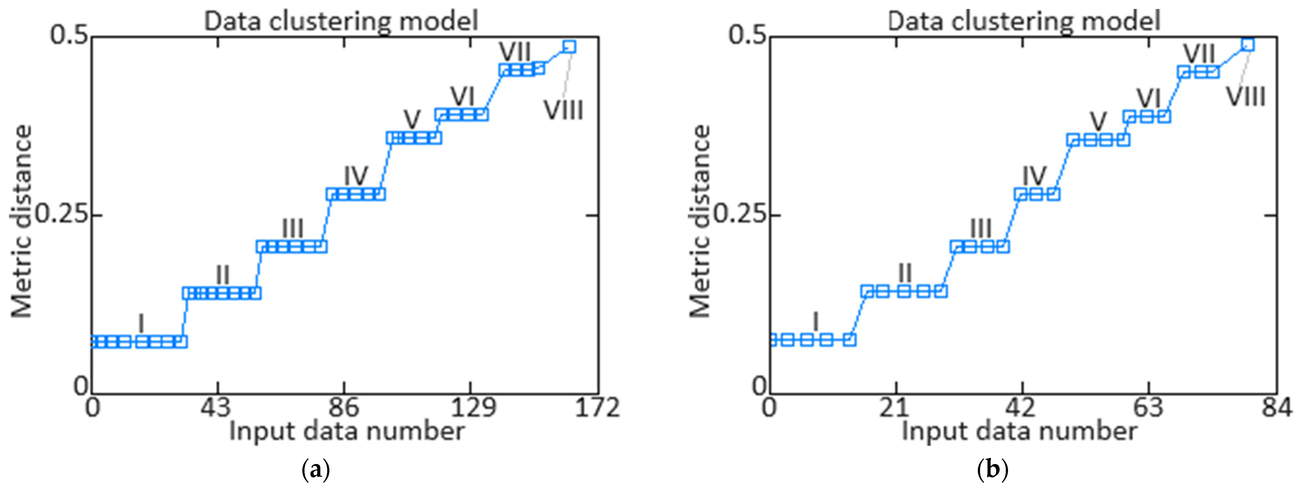
The training dataset (Table 1) homogeneity evaluation using Fisher–Pearson [46] and Fisher–Snedecor [47] criteria is detailed in [41]. According to these criteria, the training dataset of gas temperature readings before the compressor turbine for the TV3-117 aircraft engine is homogeneous, as the calculated values for the Fisher–Pearson and Fisher–Snedecor criteria are below their critical values, i.e., и . To assess the representativeness of the training dataset, ref. [41] employed cluster analysis (k-means [48,49]). Using random sampling, the training and test datasets were divided in a 2:1 ratio (67% and 33%, corresponding to 172 and 84 elements, respectively). The cluster analysis results for the training dataset (Table 1) identified eight classes (classes I …VIII), indicating the presence of eight groups and demonstrating the similarity between the training and test datasets (Figure 5).

Figure 5.
Cluster analysis results: (a) the parameter training sample, (b) the parameter test sample (author’s research, published in [41]).
These results enabled the optimal sample sizes for the determination of gas temperature before the compressor turbine for the TV3-117 aircraft engine: the training dataset comprises256 elements (100%), the validation dataset comprises 172 elements (67% of the training dataset), and the test dataset comprises84 elements (33% of the training dataset).
After the processing of data by the preprocessor, the first 172 values (67%) from the sensor (control dataset) were used in two roles: as a dataset for tuning the SARIMAX model parameters used by the reconstructor and as the training dataset for the recurrent neural network in the predictor subsystem. The remaining 84 values (33%) from the sensor (test dataset) were used for the data cleaning module operation simulated under normal conditions.
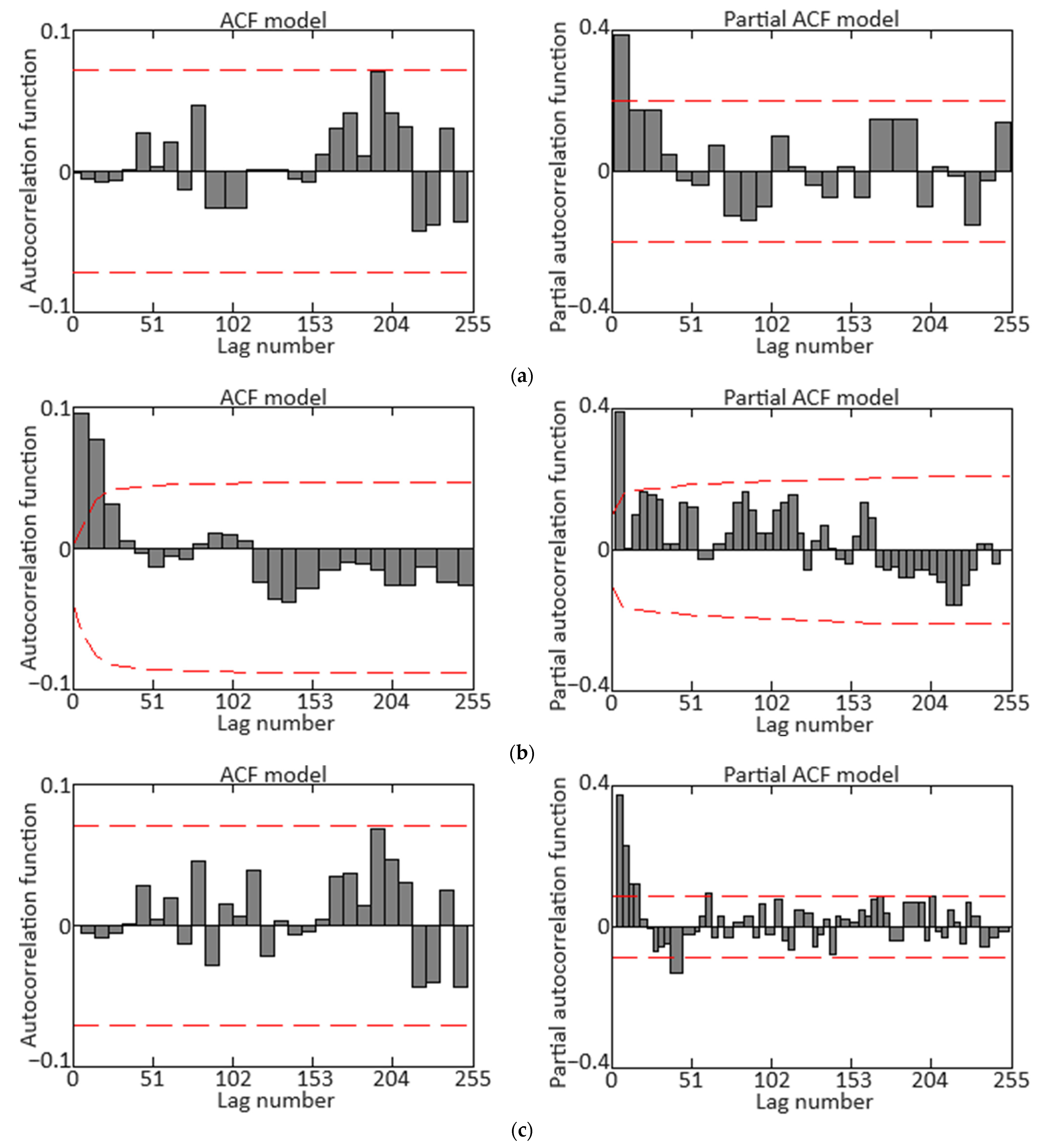
Testing the dataset with ADF and KPSS tests confirmed its non-stationarity. To achieve stationarity, techniques were sequentially applied, including first differencing to remove the trend and seasonal differencing to eliminate seasonality [50]. The corresponding autocorrelation function (ACF) and partial autocorrelation function (PACF) diagrams are shown in Figure 6. The final diagrams in Figure 6c allow for the SARIMAX model parameters’ following range selections: autoregressive order p ∈ [0, 7], differencing order d = 1, moving average order q ∈ [0, 7], seasonal autoregressive order P = 1, seasonal differencing order D = 1, seasonal moving average order Q = 0, and seasonal period s = 96.
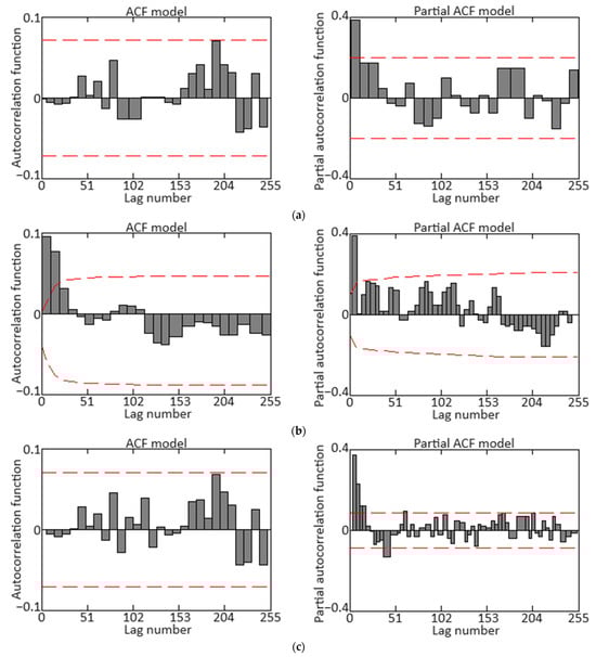
Figure 6.
Correlograms of the initial training sample readings of the gas temperature from the TV3-117 aircraft engine’s in front of the compressor turbine sensor: (a) ACF and PACF diagrams for the target time series; (b) ACF and PACF diagrams for the seasonal differences series; (c) ACF and PACF diagrams for the first differences series (author’s research).
Clarification: In the context of sensor data registration on board helicopters during flight, the term “seasonality” refers to regular and predictable changes in the data caused by time periods within the year (autumn–winter and spring–summer flights), which must be factored for accurate real-time interpretation and analysis. The impact on the sensor readings for gas temperatures before the compressor turbine in helicopter flight during the autumn–winter and spring–summer periods is linked to variations in the external temperature and pressure conditions, leading to changes in the thermodynamic properties of the air entering the engine [51,52,53]. In this research, the parameters have been adjusted for helicopter flight conditions during the spring–summer period.
In addition to accounting for “seasonality”, the calibration of the predicting system incorporates actual environmental conditions such as temperature, humidity, and atmospheric pressure. These factors significantly influence the sensor data interpretation accuracy, as they affect the engine’s thermodynamic properties and the sensor readings. By integrating these real-time environmental parameters into the calibration process, the system can more precisely adjust for variations and improve the reliability of its predictions under varying flight conditions.
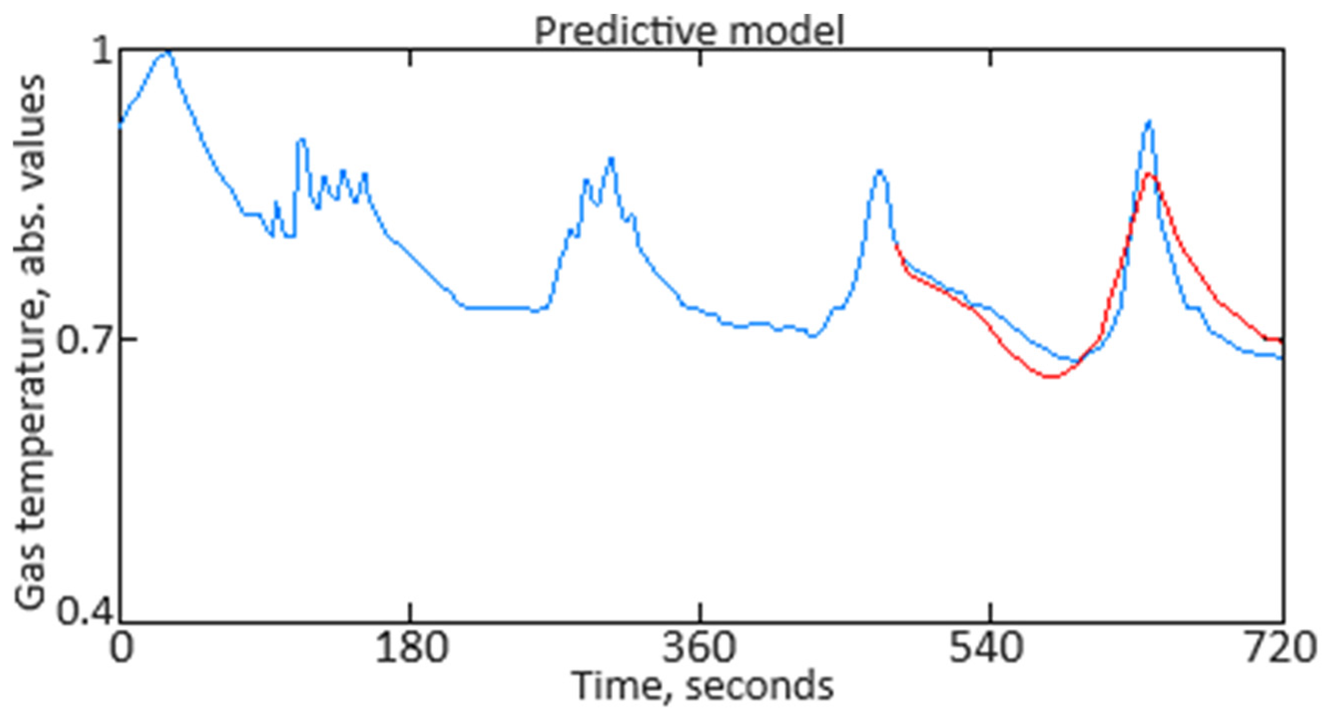
Among all the obtained models, the model with SARIMAX parameters s = 96, (p = 6, d = 1, q = 5) (P = 0, D = 1, Q = 1) was selected for the data cleaning module’s routine operation. This model was chosen due to its lowest values for the Akaike information criterion (AIC) [54] and Bayesian information criterion (BIC) [55] compared to other models, and the residual series (the difference between actual and predicted values) exhibits unbiasedness properties, stationarity, and a lack of autocorrelation. Figure 7 presents a 4 min prediction for helicopter flight, with the prediction error having an MSE = 0.218%. In Figure 7, the “blue curve” represents the actual data recorded by the sensor, and the “red curve” represents the predicted data.
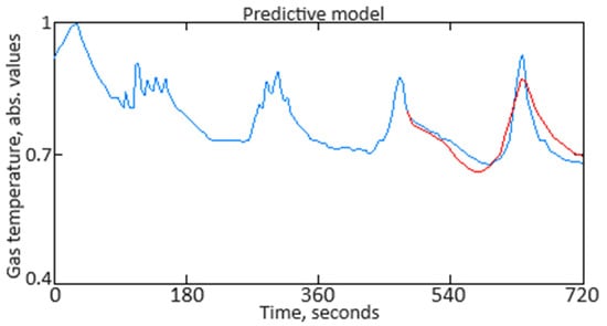
Figure 7.
The resulting diagram of the prediction readings of gas temperature from the TV3-117 aircraft engine’s in front of the compressor turbine sensor for one minute of helicopter flight, obtained using the SARIMAX model (author’s research).
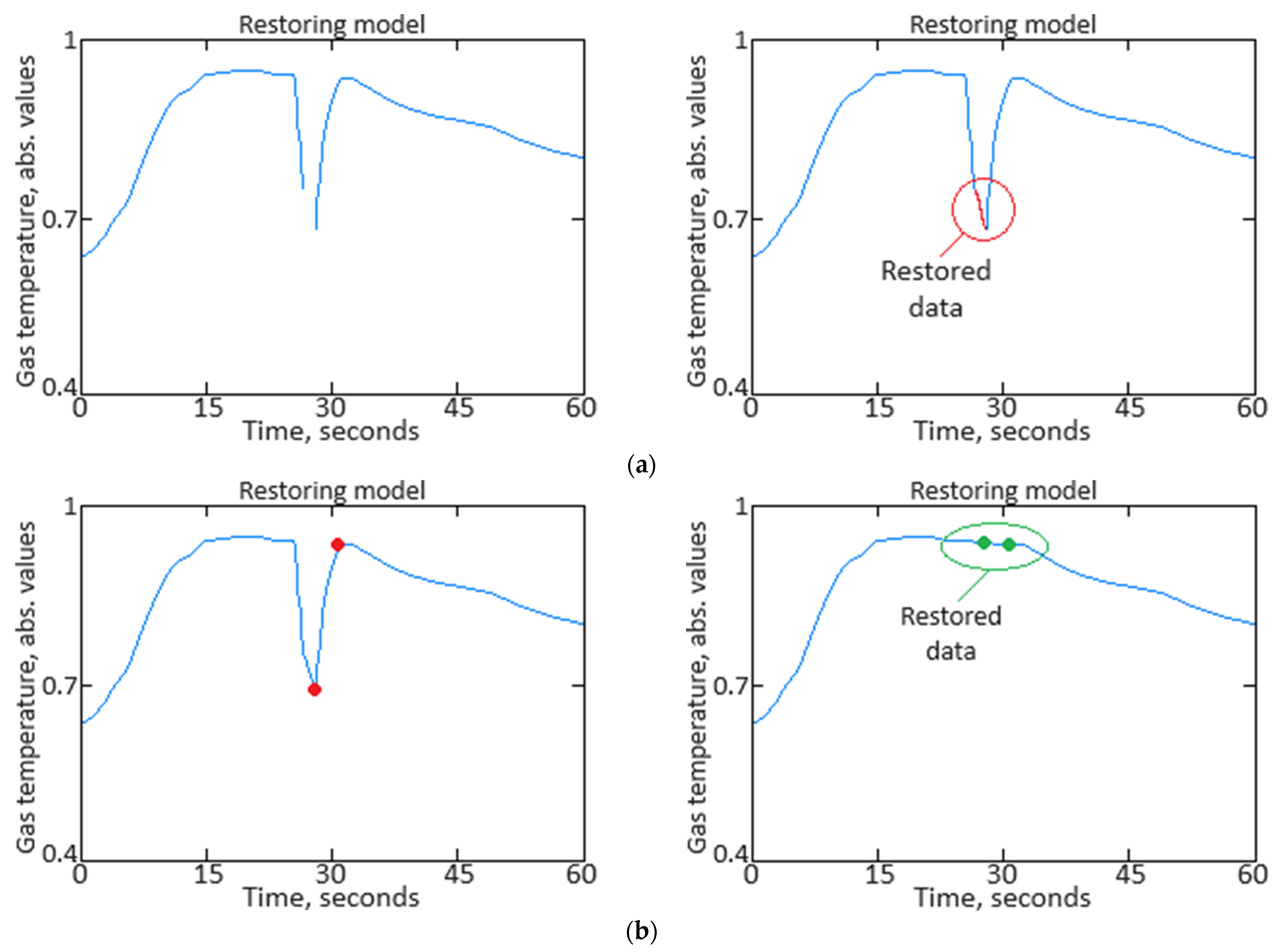
Since the proposed SARIMAX model predicts values for the gas temperature from the TV3-117 aircraft engine’s in front of the compressor turbine sensor with high accuracy, it can be used to replace missing values with plausible synthetic values. Examples of the reconstructor’s performance are shown in Figure 8. In Figure 8, the “blue curve” represents the actual data recorded by the sensor, the “red curve” represents restored data, the “red dots” indicate outliers, and the “green dots” represent imputed values.
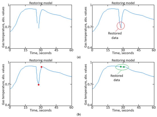
Figure 8.
The restorer’s work results based on the SARIMAX model: (a) diagram of the restoration of time series missing values; (b) diagram of the replacement of time series outliers with plausible synthetic values (author’s research).
3.2. Evaluation of Data Restoring Accuracy
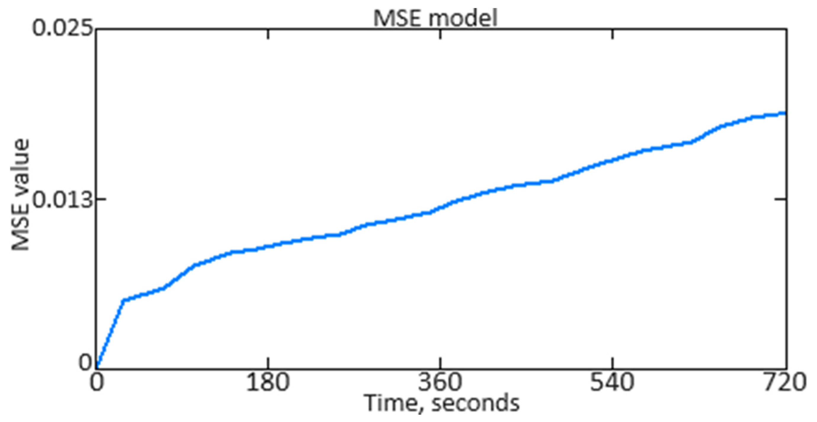
In the experiments, the TV3-117 aircraft engine gas temperature in front of the compressor turbine sensor readings, synthesized by the data cleaning module, were compared with the actual values obtained from the data repository to assess accuracy. The accuracy was measured using the MSE metric, defined as
where ti and are the actual and synthetic sensor values, respectively, and ∣B∣ denotes the sensor reading block length used for comparison. The experiments results, where the block length varied with helicopter flights from one to two minutes, are shown in Figure 9. As seen in Figure 9, the developed module ensures high and stable accuracy, with the MSE value not exceeding 0.025 (2.5%).
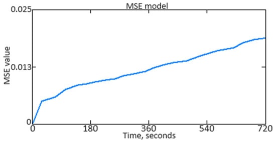
Figure 9.
Diagram of the accuracy of the data cleaner module (author’s research).
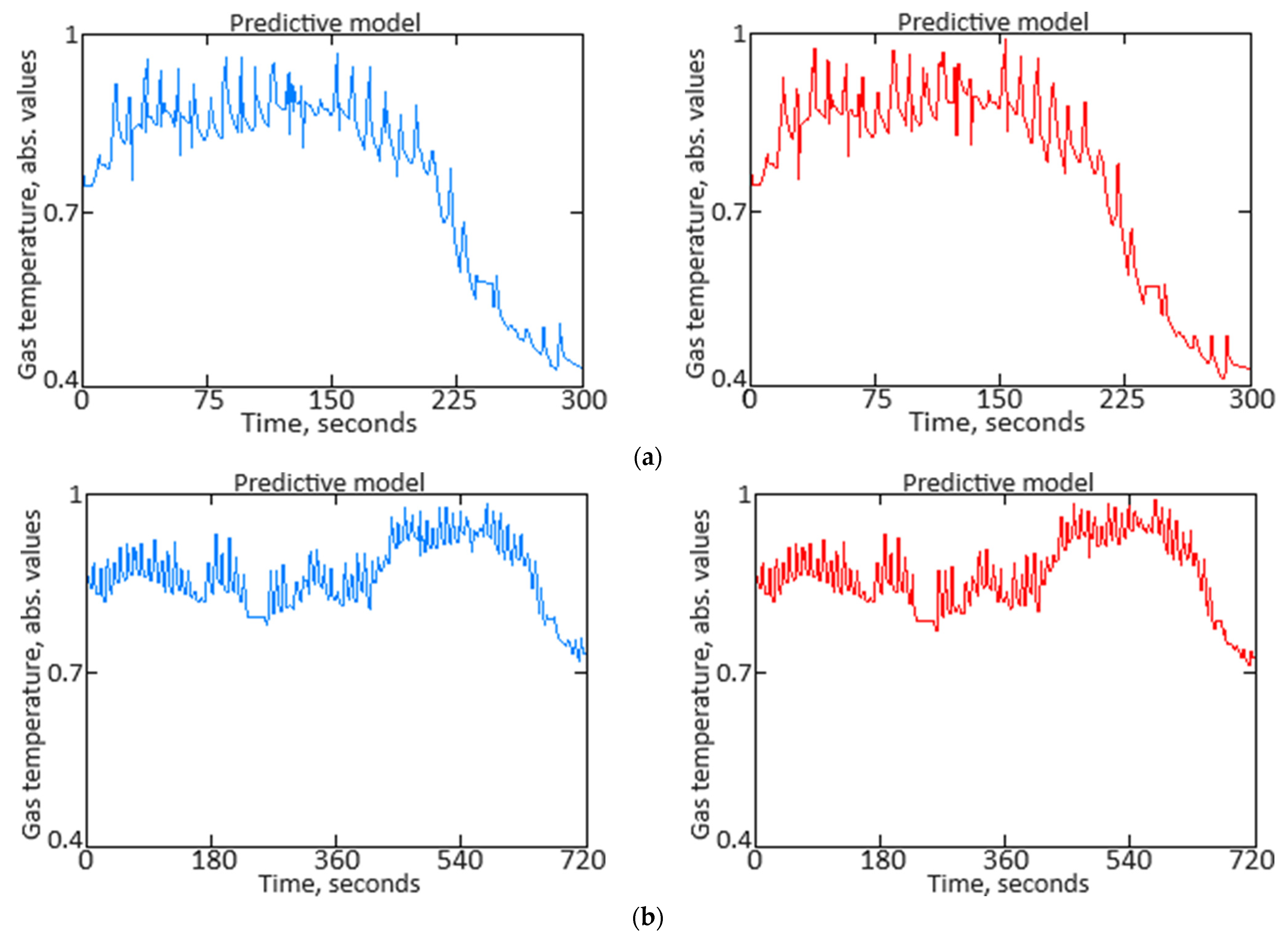
Figure 10 shows examples of the module’s operation simulation for different lengths of the sensor reading block. It can be seen from Figure 10 that the module adequately predicts normal values and detects point emissions in the data. In Figure 10, the “blue curve” represents the actual data recorded by the sensor, and the “red curve” represents the predicted data.
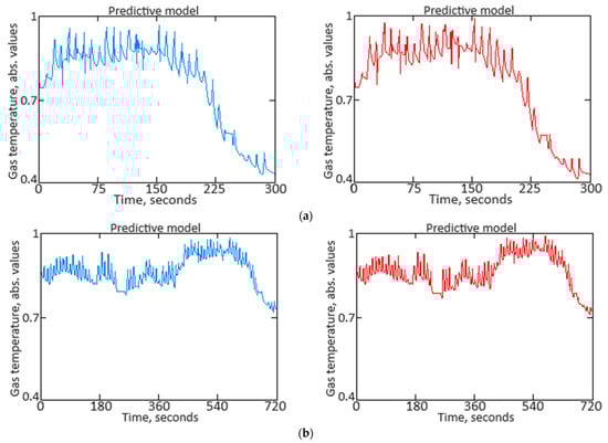
Figure 10.
Diagram of the data cleaner module’s simulation results: (a) ∣B∣ = 5 min; (b) ∣B∣ = 12 min (author’s research).
3.3. Results of Data Anomaly Prediction
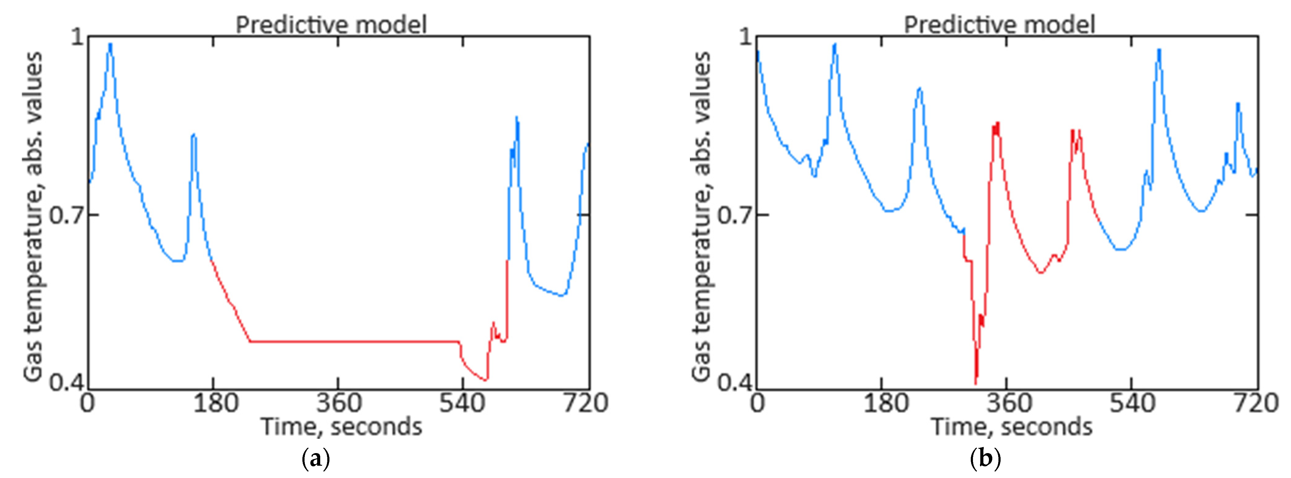
Figure 11 illustrates an example of two anomalies detected during the data cleaning module’s simulation, corresponding to two minutes of the TV3-117 aircraft engine gas temperature before the compressor turbine sensor activity under helicopter flight conditions. The first anomaly is a “Top 1 dissonance” found in the test dataset, indicating a temporary malfunction of the sensor. The second anomaly is a “Top 10 dissonance” and points to a rapid decrease in gas temperature before the compressor turbine due to increased airflow speed and changes in external air pressure. In both cases, the detected anomalies require a response from the helicopter’s flight commander (human operator). These anomalies prompt an immediate assessment by the flight commander to determine the appropriate corrective actions or adjustments needed. Such proactive responses help maintain optimal engine performance and ensure operational safety by addressing potential issues before they escalate. The system’s ability to accurately detect and classify anomalies in real time significantly enhances the reliability and responsiveness of the monitoring process.
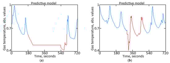
Figure 11.
Diagrams of anomalies detected during the data cleaning module’s simulation: (a) “Top 1 anomaly” (sensor activity over 12 min of helicopter flight); (b) “Top 10 anomaly” (sensor activity over 12 min of helicopter flight) (author’s research).
To better interpret the anomaly detection results, it is important to discuss both healthy and unhealthy conditions in detail. By examining the baseline or normal operational parameters alongside the detected anomalies, one can more accurately assess the system’s performance and sensitivity. Healthy conditions may include stable engine performance with consistent sensor readings and normal gas temperatures before the compressor turbine, indicative of optimal operation. Unhealthy conditions, on the other hand, might involve irregular sensor data, such as sudden temperature drops or fluctuating readings due to sensor malfunctions, increased airflow speeds, or changes in external air pressure.
To perform cross-validation (k-fold cross-validation), the training dataset is partitioned into k subsets (folds): D1, D2, …, Dk. For each i-th fold (i = 1, 2, …, k), one subset serves as the validation set while the remaining k − 1 folds are utilized for training. The model is trained on the k − 1 subsets and assessed on the remaining subset. In each i-th iteration, the model is trained on data (and evaluated on data ), where
Subsequently, the metric (in this research, MSE) is computed on the validation set for each i-th fold:
where M(i) represents a model trained on . Upon completion of all k iterations, the mean metric value is computed across all folds:
In assessing the effectiveness of the computational experiment, a cross-validation procedure (k-fold cross-validation) was performed. For this, k = 5 equal subsets (folds) of 51 elements each randomly chosen from the training sample. The following metric values were obtained: Metric(k1) = 0.224%, Metric(k2) = 0.228%, Metric(k3) = 0.227%, Metric(k4) = 0.226%, and Metric(k5) = 0.229%. The average metric was calculated as 0.227%, which differs from MSEmin = 0.218% by 3.96%. This indicates that the average value of the metric (mean square error) after cross-validation is close to the MSEmin obtained from one fold (in this case, k3). The 3.96% difference reflects how much the average metric deviates from the best individual result achieved during the cross-validation iterations. The results also suggest that the model demonstrates stability in its predictions across different data subsets (folds), as evidenced by the small difference between the average metric and MSEmin. However, it is crucial to note that the average metric offers a more generalized view of performance across the entire training set, while MSEmin highlights the optimal result obtained from a single data subset. Further analysis could investigate whether additional folds or variations in data distribution might further enhance the model’s accuracy.
3.4. Evaluation of the Effectiveness of the Results Obtained
To evaluate the effectiveness [56,57,58,59,60] of the proposed neural network system for predicting anomalous data in sensor systems (Figure 1), various metrics need to be considered, such as mean squared error (MSE) and mean absolute error (MAE), which reflect the accuracy in predicting sensor values. The determination coefficient (R2) shows how well the model explains data variations, while the correctly replaced outlier percentage and the false positive rate demonstrate the effectiveness of the reconstructor and anomaly detector. Additionally, the missed outlier rate and anomaly detection accuracy provide insight into the system’s ability to correctly identify and classify anomalies, while mean response time to anomalies assesses the system’s operational speed. In the context of a system for predicting anomalous data, Precision reflects the system’s ability to avoid false positives. This is crucial to prevent the operator from being overwhelmed by unnecessary notifications about anomalies that are actually normal data. Recall indicates how well the system can identify all existing anomalies. The F1-score is a combined metric that considers both Precision and Recall. The ROC curve displays the true positive rate (TPR) against the false positive rate (FPR) across various threshold values. These metrics enable a comprehensive evaluation, ensuring the accurate prediction and reliable detection of anomalies in sensor data. The results evaluating the effectiveness of the proposed neural network system for predicting anomalous data in sensor systems are presented in Table 2. Accordingly, the confusion matrix is given in Table 3.
Table 2.
Effectiveness evaluation results (author’s research).
Table 3.
The confusion matrix (author’s research).
True positive (TP) represents the number of cases where the system correctly identified an anomaly, that is, the system classified an event as an anomaly, and it was indeed an anomaly. True negative (TN) represents the number of cases where the system correctly identified data as normal (not an anomaly), that is, the system classified an event as normal, and it was indeed normal. False positive (FP) represents the number of false alarms where the system mistakenly classified normal data as anomalies, that is, the system identified an event as an anomaly, but it was actually not an anomaly. False negative (FN) represents the number of missed anomalies where the system did not recognize an anomaly, that is, the system classified an event as normal, but it was actually an anomaly.
A comparative analysis (Table 4) was conducted between the developed neural network system (Figure 1), a neural network system based on an autoassociative neural network (autoencoder) created by the same research team [2], and a hybrid mathematical model utilizing Runge–Kutta optimization and Bayesian hyperparameter optimization [31], according to the quality metrics presented in Table 2.
Table 4.
Comparative analysis results (author’s research).
As shown in Table 4, the quality metric values for the developed neural network system (Figure 1) and the neural network system based on the autoassociative neural network (autoencoder) [2] are approximately equal. This indicates that both systems are interchangeable and can serve as alternatives to one another. The quality metrics for the developed neural network system (Figure 1) are, on average, up to 20% higher than those of the hybrid mathematical model utilizing Runge–Kutta and Bayesian hyperparameter optimization.
For ROC analysis [57,58] across the three approaches (the developed neural network system, the neural network system based on an autoassociative neural network (autoencoder) [2], and the hybrid mathematical model utilizing Runge–Kutta optimization and Bayesian hyperparameter optimization [31]), true positive and false positive rates were calculated for each category and technique, followed by the creation of the respective ROC curves. This procedure involved defining a binary classification for each category, isolating it from the others. The ROC analysis results are presented in Table 5.
Table 5.
Comparative analysis results (author’s research).
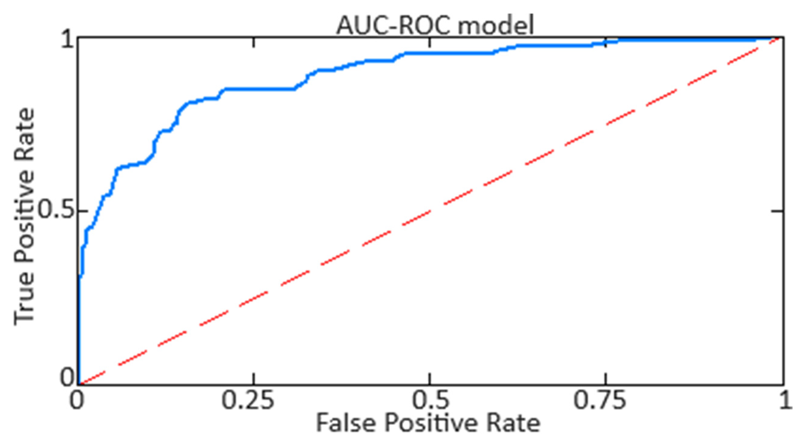
Figure 12 distinctly illustrates the variation in the regions beneath the AUC curve for the developed neural network system.
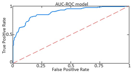
Figure 12.
AUC-ROC curve for the developed neural network system (author’s research).
Based on the obtained AUC-ROC metric values, it is noted that the developed neural network system (Figure 1) and the system based on an autoassociative neural network (autoencoder) [2] deliver high accuracy with a minimal false alarm rate. The use of the model employing Runge–Kutta and Bayesian hyperparameter optimization [31] results in lower accuracy and the highest number of false alarms.
4. Discussion
This article represents a continuation in the research field of the intelligent monitoring and operational control of helicopter TEs under onboard conditions. The proposed neural network system for anomaly prediction can function as a neural network module within the helicopter TE monitoring and operation control onboard expert system. It is well-known that predicting the helicopter TE thermogasdynamics parameters based on data obtained from standard sensors during flight is the critical aspect of helicopter flight performance. The developed system allows for real-time data analysis and decision making based on the predicted parameters, thereby enhancing the reliability and efficiency of helicopter operations. Implementing this neural network system into helicopter TE monitoring and control onboard expert systems can significantly improve the fault diagnosis and prediction quality.
By employing a modified LSTM network with a long short-term memory layer as the predictor, which also implements the reconstructor model, the developed system predicts the helicopter TE thermogasdynamics parameters with an accuracy of up to 97.9%. This allows the data cleaning module to accurately (98.2% accuracy achieved) predict normal values and detect outliers in the data. The mean squared error does not exceed 0.025 (2.5%). Although the achieved prediction accuracy of 97.9% is sufficient for asset maintenance planning, it may not be reliable enough for decision making in safety-critical operations, where higher precision and lower error margins are essential. Further refinement is needed to ensure the system’s robustness in scenarios requiring stringent operational safety [59,60] standards.
The application of the anomaly detector model in the developed system enabled the detection of two anomalies in the TV3-117 engine gas temperature before the compressor turbine sensor readings during helicopter flight, based on two minutes of sensor activity. The first anomaly (“Top 1 dissonance”) indicates a brief sensor malfunction, while the second (“Top 10 dissonance”) reflects a sharp drop in gas temperature before the compressor turbine due to increased airflow speed and changing external pressure. The false positive rate does not exceed 1.12%, the false negative rate does not exceed 1.01%, and the anomaly detection time does not exceed 1.611 s, which highlights the high efficiency of the developed system.
The AUC-ROC value of 0.818 suggests that the developed system has a strong ability to differentiate between normal and anomalous data, making it a reliable tool for accurate anomaly detection. This means the system effectively minimizes both false alarms and missed anomalies, confirming its high performance in real-world operational conditions.
The limitations related to the obtained results include the dependency on the accuracy in predicting and detecting anomalies, itself dependent on the quality of data provided by onboard sensors, which may be affected by technical malfunctions or data noise. The proposed system utilizes a modified LSTM network that demonstrates high accuracy (up to 97.9%); however, this accuracy may vary depending on helicopter operating conditions and sensor status. Additionally, the model requires significant computational resources for real-time data processing, which may limit its applicability in environments with restricted computational capacity.
The prospects for further research in the field of helicopter TE intelligent monitoring and operational control include optimizing and adapting the proposed neural network system to work with a wide range of aircraft and operational conditions. Particular interest lies in integrating various data processing methods and improving the reconstruction and prediction algorithms, which will enhance anomaly detection accuracy and speed. Additionally, exploring the potential of hybrid models that combine the strengths of the neural network and traditional approaches could lead to the creation of more robust and reliable diagnostic systems capable of operating effectively under limited computational resources and changing external factors.
Furthermore, future research prospects include conducting similar computational experiments with an expanded dataset size for generalizability and extending the on-board helicopter condition-monitoring experiment time to improve reliability.
5. Conclusions
The scientific novelty of the obtained results lies in the development of a neural network system for predicting anomalous data in sensor systems, which, through a preprocessor, predictor, reconstructor, and anomaly detector, enables anomaly prediction in sensor data with an accuracy of up to 98.2%. The scientific novelty in this article was achieved as follows:
- A preprocessor model based on the SARIMAX model was developed, allowing for the determination of autocorrelation and partial autocorrelation in the training dataset while accounting for dynamic changes (e.g., seasonal variations) and external regressors and trends, enabling time series prediction with an accuracy of up to 97.9%.
- A predictor model based on a modified LSTM network with additional Dropout and Dense layers was developed, enabling sensor-derived value prediction. An example of the prediction of TV3-117 aircraft engine gas temperature before the compressor turbine values for one minute of helicopter flight experimentally confirmed that the prediction error did not exceed 0.218%.
- A reconstructor model was developed, which, by utilizing the distribution of prediction errors, allowed for the restoration of missing time series values and outlier replacement with plausible synthetic values with an accuracy of up to 98.73%.
- An anomaly detector model was developed that, through the application of the concept of dissonance, allowed for sensor data anomaly prediction. This enabled the detection of two anomalies based on two minutes of activity from the TV3-117 aircraft engine gas temperature before the compressor turbine sensor during flight: a brief sensor malfunction and a sharp temperature drop due to changes in airflow, with type I and type II errors below 1.12 and 1.01%, respectively, and a detection time of less than 1.611 s, confirming the system’s high efficiency.
- An AUC-ROC value of 0.818 indicated that the developed system has a strong capability to distinguish between normal and anomalous data, making it a reliable tool for accurately detecting anomalies while effectively minimizing both false positives and missed detections.
Author Contributions
Conceptualization, S.V., V.V. and V.L.; methodology, S.V., M.N. and V.V.; software, V.V. and V.L.; validation, V.V. and V.L.; formal analysis, S.V.; investigation, M.N.; resources, M.N., V.S. and O.M.; data curation, S.V., M.N., V.V. and V.L.; writing—original draft preparation, S.V.; writing—review and editing, S.V.; visualization, V.V.; supervision, V.S. and O.M.; project administration, V.S. and O.M.; funding acquisition, M.N. All authors have read and agreed to the published version of the manuscript.
Funding
This research received no external funding.
Data Availability Statement
Data are contained within the article.
Acknowledgments
This research was supported by the Ministry of Internal Affairs of Ukraine as “Theoretical and applied aspects of the aviation sphere development” under Project No. 0123U104884 and by the Ministry of Education and Science of Ukraine “Methods and means of identification of combat vehicles based on deep learning technologies for automated control of target distribution” under Project No. 0124U000925.
Conflicts of Interest
The authors declare no conflict of interest.
Nomenclature
| c | is the constant; |
| φ1, …, φp | are the autoregressive coefficients; |
| θ1, …, θq | are the moving average coefficients; |
| εt | is the white noise; |
| Xt | are the exogenous regressors; |
| is the predicted value obtained using the SARIMAX model; | |
| tmin and tmax | are the minimum and maximum values in Ti,n; |
| fsensor | is the sensor frequency; |
| horizon | is the historical horizon (the time interval length in the past); |
| ct−1 | is the memory tensor at the previous time step; |
| ct | is the memory tensor at the current time step; |
| ht−1 | is the network output tensor at the previous time step; |
| ht | is the network output tensor at the current time step; |
| xt | is the input tensor at the current time step; |
| nt | is the tensor at the control unit output; |
| rt | is the tensor at the recording unit output; |
| Wcn, Whn, Wxn, Whr, Wxr, Wch, Whh, Wxh | are the weight coefficients connecting inputs to units; |
| σ | is the sigmoid function; |
| x | is the input sequence; |
| h | is the network cell hidden state vector; |
| Ui, Uf, Uo, Ug, Wi, Wf, Wo, Wg | are the network filter weight matrices for the training sequence element indices i, f, o, g, t; |
| ct | is the network cell state vector; |
| ht | is the hidden state vector; |
| m | is the mask vector created randomly with probability p; |
| p | is the probability that the element will be deactivated; |
| is the scaling factor for maintaining the activation level during training; | |
| W | is the m × n weight matrix; |
| b | is the displacement vector of size m; |
| z | is the intermediate output vector of size m; |
| μ | is the predicting error average value calculated from historical data; |
| δ | is the predicting error standard deviation calculated from historical data; |
| k | is the parameter determined by the system operator; |
| Tj,n | is the subsequence of length n starting at position j; |
| MC | is the set of all subsequences that are not trivial matches to C; |
| is the set of the k-th closest subsequence that is not a trivial match to D; | |
| is the real data average; | |
| N | is the total number of detected anomalies; |
| Tdetected,i | is the time when the i-th anomaly was detected by the system; |
| Toccurred,i | is the time when the i-th anomaly actually occurred; |
| TPreplaced | is the number of outliers that were correctly replaced by the reconstructor with predicted values; |
| FPreplaced | is the number of normal data incorrectly replaced by the reconstructor with predicted values. |
Appendix A
A modified function, mReLU(x), is proposed, which includes two parameters, α and β, that regulate sensitivity to negative and small positive values:
where α is a parameter regulating the linear relations for positive values x; β is a parameter controlling the nonlinear component for small positive values x; and γ is a parameter determining the leakage for negative values x. Parameters α, β, and γ are trained to adapt the function to specific sensor data.
The nonlinear element β · x2 in (A1) allows the function to be more sensitive to small deviations in positive values, which can be useful for detecting minor but important deviations that may indicate a potential anomaly. Considering that some anomalies may manifest in negative values, the parameter γ enables control over how much the negative values are reduced. It is assumed that anomalies are detected when the function’s values exceed the allowable range. In this case, an anomaly function A(x) can be introduced:
where T1 and T2 are the upper and lower thresholds for the normal values of the output function.
If sensor data x is fed into a neural network activated by the function mReLU(x), the output mReLU(x) can be compared to the thresholds T1 and T2 for real-time anomaly detection. Parameters α, β, and γ are adjusted during the network training to ensure the function optimally responds to specific anomalies in the data.
References
- Diao, H.; Yin, L.; Liang, B.; Chen, Y. An Intelligent System Control Method Based on Visual Sensor. Measurement. Sensors 2023, 29, 100857. [Google Scholar] [CrossRef]
- Vladov, S.; Yakovliev, R.; Vysotska, V.; Nazarkevych, M.; Lytvyn, V. The Method of Restoring Lost Information from Sensors Based on Auto-Associative Neural Networks. Appl. Syst. Innov. 2024, 7, 53. [Google Scholar] [CrossRef]
- Lyu, K.; Tan, X.; Liu, G.; Zhao, C. Sensor Selection of Helicopter Transmission Systems Based on Physical Model and Sensitivity Analysis. Chin. J. Aeronaut. 2014, 27, 643–654. [Google Scholar] [CrossRef]
- Selivanova, K.; Avrunin, O.; Tymkovych, M.; Manhora, T.; Bezverkhyi, O.; Omiotek, Z.; Kalizhanova, A.; Kozbakova, A. 3D Visualization of Human Body Internal Structures Surface during Stereo-Endoscopic Operations Using Computer Vision Techniques. Przegląd Elektrotechniczny 2021, 9, 32–35. [Google Scholar] [CrossRef]
- Avrunin, O.; Nosova, Y.; Younouss Abdelhamid, I.; Gryshkov, O.; Glasmacher, B. Using 3d printing technology to full-scale simulation of the upper respiratory tract. Inform. Autom. Pomiary W Gospod. I Ochr. Sr. 2019, 9, 60–63. [Google Scholar] [CrossRef]
- Zagirnyak, M.V.; Prus, V.V.; Somka, O.; Dolezel, I. Models of Reliability Prediction of Electric Machine Taking into Account the State of Major Structural Units. Adv. Electr. Electron. Eng. 2015, 13, 447–452. [Google Scholar] [CrossRef]
- Baranovskyi, D.; Myamlin, S. The Criterion of Development of Processes of the Self-Organization of Subsystems of the Second Level in Tribosystems of Diesel Engine. Sci. Rep. 2023, 13, 5736. [Google Scholar] [CrossRef]
- Andriushchenko, K.; Rudyk, V.; Riabchenko, O.; Kachynska, M.; Marynenko, N.; Shergina, L.; Kovtun, V.; Tepliuk, M.; Zhemba, A.; Kuchai, O. Processes of managing information infrastructure of a digital enterprise in the framework of the «Industry 4.0» concept. East.-Eur. J. Enterp. Technol. 2019, 1, 60–72. [Google Scholar] [CrossRef]
- Yang, L. Measurement of High Quality Development of Manufacturing Industry Empowered by Big Data Based on Intelligent Sensor Systems. Meas. Sens. 2024, 33, 101092. [Google Scholar] [CrossRef]
- Cui, W.; Chen, Y.; Xu, B. Application Research of Intelligent System Based on BIM and Sensors Monitoring Technology in Construction Management. Phys. Chem. Earth Parts A/B/C 2024, 134, 103546. [Google Scholar] [CrossRef]
- Vladov, S.; Shmelov, Y.; Yakovliev, R. Method for Forecasting of Helicopters Aircraft Engines Technical State in Flight Modes Using Neural Networks. CEUR Workshop Proc. 2022, 3171, 974–985. Available online: https://ceur-ws.org/Vol-3171/paper70.pdf (accessed on 12 July 2024).
- Keum, K.; Kwak, J.Y.; Rim, J.; Byeon, D.H.; Kim, I.; Moon, J.; Park, S.K.; Kim, Y.-H. Dual-Stream Deep Learning Integrated Multimodal Sensors for Complex Stimulus Detection in Intelligent Sensory Systems. Nano Energy 2024, 122, 109342. [Google Scholar] [CrossRef]
- Lai, L.; Gaohua, Z. Intelligent Speech Elderly Rehabilitation Learning Assistance System Based on Deep Learning and Sensor Networks. Meas. Sens. 2024, 33, 101191. [Google Scholar] [CrossRef]
- Cheng, K.; Wang, Y.; Yang, X.; Zhang, K.; Liu, F. An Intelligent Online Fault Diagnosis System for Gas Turbine Sensors Based on Unsupervised Learning Method LOF and KELM. Sens. Actuators A Phys. 2024, 365, 114872. [Google Scholar] [CrossRef]
- Kumar, S.R.; Devakumar, J. Recurrent Neural Network Based Sensor Fault Detection and Isolation for Nonlinear Systems: Application in PWR. Prog. Nucl. Energy 2023, 163, 104836. [Google Scholar] [CrossRef]
- Alghamdi, W.Y. A Novel Deep Learning Method for Predicting Athletes’ Health Using Wearable Sensors and Recurrent Neural Networks. Decis. Anal. J. 2023, 7, 100213. [Google Scholar] [CrossRef]
- Hrytsyk, V.; Medykovskyy, M.; Nazarkevych, M. Estimation of Symmetry in the Recognition System with Adaptive Application of Filters. Symmetry 2022, 14, 903. [Google Scholar] [CrossRef]
- Sok, R.; Jeyamoorthy, A.; Kusaka, J. Novel Virtual Sensors Development Based on Machine Learning Combined with Convolutional Neural-Network Image Processing-Translation for Feedback Control Systems of Internal Combustion Engines. Appl. Energy 2024, 365, 123224. [Google Scholar] [CrossRef]
- Sarwar, U.; Muhammad, M.; Mokhtar, A.A.; Khan, R.; Behrani, P.; Kaka, S. Hybrid Intelligence for Enhanced Fault Detection and Diagnosis for Industrial Gas Turbine Engine. Results Eng. 2024, 21, 101841. [Google Scholar] [CrossRef]
- Vladov, S.; Yakovliev, R.; Hubachov, O.; Rud, J.; Stushchanskyi, Y. Neural Network Modeling of Helicopters Turboshaft Engines at Flight Modes Using an Approach Based on “Black Box” Models. CEUR Workshop Proc. 2024, 3624, 116–135. Available online: https://ceur-ws.org/Vol-3624/Paper_11.pdf (accessed on 21 July 2024).
- Wang, G.; Zhao, J.; Yang, J.; Jiao, J.; Xie, J.; Feng, F. Multivariate Statistical Analysis Based Cross Voltage Correlation Method for Internal Short-Circuit and Sensor Faults Diagnosis of Lithium-Ion Battery System. J. Energy Storage 2023, 62, 106978. [Google Scholar] [CrossRef]
- Badura, M.; Szczurek, A.; Szecówka, P.M. Statistical Assessment of Quantification Methods Used in Gas Sensor System. Sens. Actuators B Chem. 2013, 188, 815–823. [Google Scholar] [CrossRef]
- Alwan, A.A.; Brimicombe, A.J.; Ciupala, M.A.; Ghorashi, S.A.; Baravalle, A.; Falcarin, P. Time-Series Clustering for Sensor Fault Detection in Large-Scale Cyber–Physical Systems. Comput. Netw. 2022, 218, 109384. [Google Scholar] [CrossRef]
- Boem, F.; Reci, R.; Cenedese, A.; Parisini, T. Distributed Clustering-Based Sensor Fault Diagnosis for HVAC Systems. IFAC-Pap. 2017, 50, 4197–4202. [Google Scholar] [CrossRef]
- Kayode Saheed, Y.; Harazeem Abdulganiyu, O.; Ait Tchakoucht, T. A Novel Hybrid Ensemble Learning for Anomaly Detection in Industrial Sensor Networks and SCADA Systems for Smart City Infrastructures. J. King Saud Univ.-Comput. Inf. Sci. 2023, 35, 101532. [Google Scholar] [CrossRef]
- Chang, V.; Martin, C. An Industrial IoT Sensor System for High-Temperature Measurement. Comput. Electr. Eng. 2021, 95, 107439. [Google Scholar] [CrossRef]
- Marakhimov, A.R.; Khudaybergenov, K.K. Approach to the synthesis of neural network structure during classification. Int. J. Comput. 2020, 19, 20–26. [Google Scholar] [CrossRef]
- Vladov, S.; Shmelov, Y.; Yakovliev, R.; Petchenko, M. Neural Network Method for Parametric Adaptation Helicopters Turboshaft Engines On-Board Automatic Control System Parameters. CEUR Workshop Proc. 2023, 3403, 179–195. Available online: https://ceur-ws.org/Vol-3403/paper15.pdf (accessed on 29 July 2024).
- Shabbir, W.; Aijun, L.; Yuwei, C. Neural Network-Based Sensor Fault Estimation and Active Fault-Tolerant Control for Uncertain Nonlinear Systems. J. Frankl. Inst. 2023, 360, 2678–2701. [Google Scholar] [CrossRef]
- Trapani, N.; Longo, L. Fault Detection and Diagnosis Methods for Sensors Systems: A Scientific Literature Review. IFAC-Pap. 2023, 56, 1253–1263. [Google Scholar] [CrossRef]
- Yu, Z.; Zhang, Z.; Jiang, Q.; Yan, X. Neural Network-Based Hybrid Modeling Approach Incorporating Bayesian Optimization with Industrial Soft Sensor Application. Knowl.-Based Syst. 2024, 301, 112341. [Google Scholar] [CrossRef]
- Li, C.; Yang, X. Neural Networks-Based Command Filtering Control for a Table-Mount Experimental Helicopter. J. Frankl. Inst. 2021, 358, 321–338. [Google Scholar] [CrossRef]
- Elamin, N.; Fukushige, M. Modeling and Forecasting Hourly Electricity Demand by SARIMAX with Interactions. Energy 2018, 165, 257–268. [Google Scholar] [CrossRef]
- Tarsitano, A.; Amerise, I.L. Short-Term Load Forecasting Using a Two-Stage Sarimax Model. Energy 2017, 133, 108–114. [Google Scholar] [CrossRef]
- Charemza, W.W.; Syczewska, E.M. Joint Application of the Dickey-Fuller and KPSS Tests. Econ. Lett. 1998, 61, 17–21. [Google Scholar] [CrossRef]
- Chen, Y.; Pun, C.S. A Bootstrap-Based KPSS Test for Functional Time Series. J. Multivar. Anal. 2019, 174, 104535. [Google Scholar] [CrossRef]
- Vladov, S.; Shmelov, Y.; Yakovliev, R. Methodology for Control of Helicopters Aircraft Engines Technical State in Flight Modes Using Neural Networks. CEUR Workshop Proc. 2022, 3137, 108–125. [Google Scholar] [CrossRef]
- Greff, K.; Srivastava, R.K.; Koutnik, J.; Steunebrink, B.R.; Schmidhuber, J. LSTM: A Search Space Odyssey. IEEE Trans. Neural Netw. Learn. Syst. 2017, 28, 2222–2232. [Google Scholar] [CrossRef]
- Sakata, A. Prediction Errors for Penalized Regressions Based on Generalized Approximate Message Passing. J. Phys. A Math. Theor. 2023, 56, 043001. [Google Scholar] [CrossRef]
- Zhao, X.; Fang, Y.; Min, H.; Wu, X.; Wang, W.; Teixeira, R. Potential Sources of Sensor Data Anomalies for Autonomous Vehicles: An Overview from Road Vehicle Safety Perspective. Expert Syst. Appl. 2024, 236, 121358. [Google Scholar] [CrossRef]
- Vladov, S.; Scislo, L.; Sokurenko, V.; Muzychuk, O.; Vysotska, V.; Osadchy, S.; Sachenko, A. Neural Network Signal Integration from Thermogas-Dynamic Parameter Sensors for Helicopters Turboshaft Engines at Flight Operation Conditions. Sensors 2024, 24, 4246. [Google Scholar] [CrossRef] [PubMed]
- Ferreira, L.; Moreira, G.; Hosseini, M.; Lage, M.; Ferreira, N.; Miranda, F. Assessing the Landscape of Toolkits, Frameworks, and Authoring Tools for Urban Visual Analytics Systems. Comput. Graph. 2024, 123, 104013. [Google Scholar] [CrossRef]
- Khan, A.Q.; El Jaouhari, S.; Tamani, N.; Mroueh, L. Knowledge-Based Anomaly Detection: Survey, Challenges, and Future Directions. Eng. Appl. Artif. Intell. 2024, 136, 108996. [Google Scholar] [CrossRef]
- Zare, F.; Mahmoudi-Nasr, P.; Yousefpour, R. A Real-Time Network Based Anomaly Detection in Industrial Control Systems. Int. J. Crit. Infrastruct. Prot. 2024, 45, 100676. [Google Scholar] [CrossRef]
- Amaral, M.; Signoretti, G.; Silva, M.; Silva, I. TAC: A Python Package for IoT-Focused Tiny Anomaly Compression. SoftwareX 2024, 26, 101747. [Google Scholar] [CrossRef]
- Balakrishnan, N.; Voinov, V.; Nikulin, M.S. Chapter 2—Pearson’s Sum and Pearson-Fisher Test. In Chi-Squared Goodness of Fit Tests with Applications; Balakrishnan, N., Voinov, V., Nikulin, M.S., Eds.; Academic Press: Waltham, MA, USA, 2013; pp. 11–26. [Google Scholar] [CrossRef]
- Avram, F.; Leonenko, N.N.; Šuvak, N. Hypothesis testing for Fisher–Snedecor diffusion. J. Stat. Plan. Inference 2012, 142, 2308–2321. [Google Scholar] [CrossRef]
- Hu, Z.; Kashyap, E.; Tyshchenko, O.K. GEOCLUS: A Fuzzy-Based Learning Algorithm for Clustering Expression Datasets. Lect. Notes Data Eng. Commun. Technol. 2022, 134, 337–349. [Google Scholar] [CrossRef]
- Babichev, S.; Krejci, J.; Bicanek, J.; Lytvynenko, V. Gene expression sequences clustering based on the internal and external clustering quality criteria. In Proceedings of the 2017 12th International Scientific and Technical Conference on Computer Sciences and Information Technologies (CSIT), Lviv, Ukraine, 5–8 September 2017. [Google Scholar] [CrossRef]
- Vladov, S.; Yakovliev, R.; Bulakh, M.; Vysotska, V. Neural Network Approximation of Helicopter Turboshaft Engine Parameters for Improved Efficiency. Energies 2024, 17, 2233. [Google Scholar] [CrossRef]
- Cherrat, E.M.; Alaoui, R.; Bouzahir, H. Score fusion of finger vein and face for human recognition based on convolutional neural network model. Int. J. Comput. 2020, 19, 11–19. [Google Scholar] [CrossRef]
- Hu, Z.; Dychka, I.; Potapova, K.; Meliukh, V. Augmenting Sentiment Analysis Prediction in Binary Text Classification through Advanced Natural Language Processing Models and Classifiers. Int. J. Inf. Technol. Comput. Sci. 2024, 16, 16–31. [Google Scholar] [CrossRef]
- Vladov, S.; Shmelov, Y.; Yakovliev, R. Optimization of Helicopters Aircraft Engine Working Process Using Neural Networks Technologies. CEUR Workshop Proc. 2022, 3171, 1639–1656. Available online: https://ceur-ws.org/Vol-3171/paper117.pdf (accessed on 10 August 2024).
- Morozov, V.V.; Kalnichenko, O.V.; Mezentseva, O.O. The method of interaction modeling on basis of deep learning the neural networks in complex IT-projects. Int. J. Comput. 2020, 19, 88–96. [Google Scholar] [CrossRef]
- Romanova, T.E.; Stetsyuk, P.I.; Chugay, A.M.; Shekhovtsov, S.B. Parallel Computing Technologies for Solving Optimization Problems of Geometric Design. Cybern. Syst. Anal. 2019, 55, 894–904. [Google Scholar] [CrossRef]
- Pasieka, M.; Grzesik, N.; Kuźma, K. Simulation modeling of fuzzy logic controller for aircraft engines. Int. J. Comput. 2017, 16, 27–33. [Google Scholar] [CrossRef]
- Vladov, S.; Yakovliev, R.; Hubachov, O.; Rud, J. Neuro-Fuzzy System for Detection Fuel Consumption of Helicopters Turboshaft Engines. CEUR Workshop Proc. 2022, 3628, 55–72. Available online: https://ceur-ws.org/Vol-3628/paper5.pdf (accessed on 12 September 2024).
- Lee, J.; van Es, N.; Takada, T.; Klok, F.A.; Geersing, G.-J.; Blume, J.; Bossuyt, P.M. Covariate-Specific ROC Curve Analysis Can Accommodate Differences between Covariate Subgroups in the Evaluation of Diagnostic Accuracy. J. Clin. Epidemiol. 2023, 160, 14–23. [Google Scholar] [CrossRef]
- Vladov, S.; Shmelov, Y.; Yakovliev, R.; Petchenko, M.; Drozdova, S. Neural Network Method for Helicopters Turboshaft Engines Working Process Parameters Identification at Flight Modes. In Proceedings of the 2022 IEEE 4th International Conference on Modern Electrical and Energy System (MEES), Kremenchuk, Ukraine, 20–22 October 2022. [Google Scholar] [CrossRef]
- Alozie, O.; Li, Y.-G.; Wu, X.; Shong, X.; Ren, W. An Adaptive Model-Based Framework for Prognostics of Gas Path Faults in Aircraft Gas Turbine Engines. Int. J. Progn. Health Manag. 2019, 10. [Google Scholar] [CrossRef]
Disclaimer/Publisher’s Note: The statements, opinions and data contained in all publications are solely those of the individual author(s) and contributor(s) and not of MDPI and/or the editor(s). MDPI and/or the editor(s) disclaim responsibility for any injury to people or property resulting from any ideas, methods, instructions or products referred to in the content. |
© 2024 by the authors. Published by MDPI on behalf of the International Institute of Knowledge Innovation and Invention. Licensee MDPI, Basel, Switzerland. This article is an open access article distributed under the terms and conditions of the Creative Commons Attribution (CC BY) license (https://creativecommons.org/licenses/by/4.0/).