Randomized Feature and Bootstrapped Naive Bayes Classification

Abstract

Naive Bayes (NB) classifiers are widely used for their simplicity, computational efficiency, and interpretability. However, their predictive performance can degrade significantly in real-world settings where the conditional independence assumption is often violated. More complex NB variants address this issue but typically introduce structural complexity or require explicit dependency modeling, limiting their scalability and transparency. This study proposes two lightweight ensemble-based extensions—randomized feature naive Bayes (RF-NB) and randomized feature bootstrapped naive Bayes (RFB-NB)—designed to enhance robustness and predictive stability without altering the underlying NB model. By integrating randomized feature selection and bootstrap resampling, these methods implicitly reduce feature dependence and noise-induced variance. Evaluation across twenty real-world datasets spanning medical, financial, and industrial domains demonstrates that RFB-NB consistently outperformed classical NB, RF-NB, and k-nearest neighbor in several cases. Although random forest achieved higher average accuracy overall, RFB-NB demonstrated comparable accuracy with notably lower variance and improved predictive stability specifically in datasets characterized by high noise levels, large dimensionality, or significant class imbalance. These findings underscore the practical and complementary advantages of RFB-NB in challenging classification scenarios.

1. Introduction

Machine learning has witnessed significant growth in recent decades, with the naive Bayes (NB) classifier remaining a fundamental method within probabilistic learning. Its simplicity, computational efficiency, and interpretability make NB particularly attractive for diverse applications, including text classification and medical diagnostics [1,2,3]. Despite these advantages and its solid theoretical foundations [4,5], the classifier’s assumption of conditional independence among features frequently constrains its performance in real-world settings, where this assumption seldom holds [6,7]. To address this limitation, numerous enhancements such as feature selection, parameter optimization, and hybrid modeling have been extensively explored [8,9,10,11].

Feature selection improves classification by using the most relevant features, reducing data dimensionality, and preventing model overfitting. Decision trees [8], correlation-based selection [12], and wrapper methods [10] are widely recognized techniques for this purpose. Ratanamahatana and Gunopulos [8] illustrated how decision trees effectively guide feature selection in NB classifiers, paving the way for subsequent advancements. Similarly, Kohavi and John [10] emphasized wrapper methods’ ability to directly assess subsets of features based on their predictive capabilities, establishing this as a robust selection strategy. Hall [12] demonstrated the efficacy of correlation-based selection in filtering redundant features from high-dimensional data. Extending these contributions, May et al. [13] successfully applied recursive feature elimination to NB in crime prediction contexts. Pujianto et al. [14] further compared NB and random forests, highlighting the relative strengths and limitations of these classifiers in practical news popularity prediction tasks. Additionally, Aridas et al. [15] integrated NB within random forests to enrich ensemble diversity and enhance predictive accuracy across heterogeneous datasets.

In parallel, bootstrap sampling methods have proven valuable for enhancing model robustness. Initially introduced by Efron and Tibshirani [16], bootstrap sampling offers a rigorous mechanism to estimate statistical accuracy and model variability. Integration into machine learning has inspired innovations such as bagging and ensemble learning approaches [17,18]. A notable example is the random forest (RF), proposed by Breiman [17], which merges bootstrap sampling with randomized feature selection to yield highly robust classifiers. Liaw and Wiener [19] illustrated RF’s practical efficacy, solidifying its role as a benchmark classifier. Similarly, ensemble techniques leveraging bootstrap methods, such as weighted and tree-augmented NB classifiers, have demonstrated improvements in predictive accuracy and stability [20]. Additionally, randomized kernel k-nearest neighbor (KNN) regression exemplifies the versatility of bootstrap-enhanced ensemble methods [21]. Furthermore, bootstrap methods facilitate the construction of confidence intervals for complex statistical models, including zero-truncated Poisson–Ishita distributions [22].

Another critical enhancement targets NB’s simplifying assumption of conditional feature independence. Prior studies [4,5] investigated scenarios wherein this assumption significantly undermines predictive accuracy. To alleviate such challenges, Jiang et al. [23] introduced hidden NB, employing latent variables to model dependencies among features more effectively. Similarly, other approaches [6] relaxed the independence assumption by explicitly incorporating feature correlations into NB, enhancing its adaptability. Additionally, sparse feature selection techniques [9] have been explored to improve NB performance within resource-constrained scenarios. A comprehensive review by Guyon and Elisseeff [24] further underscored the critical role of feature selection methodologies in optimizing model accuracy and interpretability.

Advanced Bayesian variants have also emerged to address NB’s independence assumption limitations, including tree-augmented naive Bayes (TAN), which explicitly models feature dependencies using Bayesian networks [25], and weighted naive Bayes (WNB), which assigns discriminative weights to features based on information gain or chi-squared metrics [26,27]. Although these methods improve classification performance, they incur increased computational complexity due to explicit dependency modeling or feature weight optimization.

Motivated by these methodological gaps, this study introduces randomized feature naive Bayes (RF-NB) and randomized feature bootstrapped naive Bayes (RFB-NB). These novel classifiers employ randomized feature selection and bootstrap aggregation, enhancing robustness and predictive stability without explicitly modeling feature dependencies or assigning fixed feature weights. Thus, our proposed methods offer computational efficiency and robust predictive performance, particularly advantageous in noisy, heterogeneous, or high-dimensional datasets. This research specifically aims to investigate whether randomized feature selection and bootstrap aggregation can significantly enhance NB classifier performance and to rigorously assess how these proposed methods compare to established classifiers across diverse real-world datasets.

The primary contributions of this study include introducing two ensemble-based naive Bayes classifiers—RF-NB and RFB-NB—that effectively mitigate the limitations imposed by the independence assumption without explicitly modeling feature dependencies and rigorously justifying their enhanced robustness and predictive stability through a theoretical explanation and focused empirical validation beyond traditional accuracy and F1-score evaluations. The manuscript is structured as follows: Section 2 reviews the relevant literature on enhancements to naive Bayes classifiers, feature selection methods, and bootstrap aggregation techniques. Section 3 details the proposed RF-NB and RFB-NB methodologies, covering theoretical formulation, algorithmic implementation, and computational considerations. Section 4 describes the datasets used for performance evaluation, emphasizing their characteristics and practical relevance. Section 5 systematically presents the empirical results, comparing RF-NB and RFB-NB performance against established benchmark classifiers. Finally, Section 6 concludes by summarizing the key findings of this research.

2. Related Theory

Naive Bayes is a probabilistic classifier that leverages Bayes’ theorem to assign a class label to an instance based on observed features. It assumes the conditional independence of features given the class label, which simplifies computation and enables efficient handling of high-dimensional data. Let $X=\left(X_1,X_2,\mathrm{\dots },X_n\right)$ represent the feature vector with n features and denote the feature vector, and let $Y\in \left\{y_1,y_2,\mathrm{\dots },y_K\right\}$ denote the target class variable with $K$ possible classes. Given a dataset of $N$ total observations, the naive Bayes classifier is trained using $N_{tr}$ observations and is tested on $N_{te}$ observations, where $N=N_{tr}+N_{te}$.

According to Bayes’ theorem, the posterior probability of a class $Y=y_k$ given the feature vector $X$ is expressed as

$$P(Y=y_k|X)={\displaystyle \frac{P(X|Y=y_k)P(Y=y_k)}{P(X)}},$$

(1)

where $P(Y=y_k)$ is the prior probability of class $y_k$, $P(X|Y=y_k)$ is the likelihood of observing $X$ given $Y=y_k,$ and $P(X)$ is the marginal likelihood of $X.$ Since $P(X)$ is constant for all classes during classification, it can be omitted.

To simplify computation, naive Bayes assumes that all features $X_i$ are conditionally independent given the class $Y.$ Thus, the likelihood $P(X|Y=y_k)$ can be factorized as

$$P(X|Y=y_k)={\displaystyle \prod _{i=1}^{n}P(X_i|Y=y_k)}.$$

(2)

This results in the posterior probability [7,28] are

$$P(Y=y_k|X)\propto P(Y=y_k){\displaystyle \prod _{i=1}^{n}P(X_i|Y=y_k)}.$$

(3)

The naive Bayes decision rule selects the class $y_k$ that maximizes the posterior probability:

$$Y=\arg \underset{y_k}{\max }P(Y=y_k){\displaystyle \prod _{i=1}^{n}P(X_i|Y=y_k)}.$$

(4)

In practice, logarithms are used to avoid numerical underflow when computing the product of probabilities:

$$\log P(Y=y_k|X)=\log P(Y=y_k)+{\displaystyle \sum _{i=1}^n\log P(X_i|Y=y_k)}.$$

(5)

2.1. Gaussian Naive Bayes

For continuous features, Gaussian naive Bayes assumes that each feature $X_i$ follows a normal (Gaussian) distribution conditional on the class $Y=y_k$. The likelihood $P(X_i|Y=y_k)$ is modeled as [29]

$$P(X_i|Y=y_k)={\displaystyle \frac{1}{\sqrt{2\pi {\sigma }_{ik}^2}}}\exp \left({\displaystyle \frac{-{\left(X_i-{\mu }_{ik}\right)}^2}{2{\sigma }_{ik}^2}}\right),$$

(6)

where ${\mu }_{ik}$ and ${\sigma }_{ik}^2$ are the mean and variance of feature $X_i$ for class $y_k$. These parameters are estimated from the training dataset, with the mean and variance computed as

$${\mu }_{ik}={\displaystyle \frac{1}{N_k}}{\displaystyle \sum _{j=1}^{N_k}{X}_i^{(j)}},\hspace{0.33em}\hspace{1em}{\sigma }_{ik}^2={\displaystyle \frac{1}{N_k}}{\displaystyle \sum _{j=1}^{N_k}{\left(X_i^{(j)}-{\mu }_{ik}\right)}^2},$$

(7)

where $N_k$ is the number of training samples in class $y_k$ and $X_i^{(j)}$ denotes the $i-$th feature value of the $j-$th training sample. The posterior probability for Gaussian naive Bayes becomes

$$P(Y=y_k|X)\propto P(Y=y_k){\displaystyle \prod _{i=1}^n\frac{1}{\sqrt{2\pi {\sigma }_{ik}^2}}\exp \left(\frac{-{\left(X_i-{\mu }_{ik}\right)}^2}{2{\sigma }_{ik}^2}\right)}.$$

(8)

Using logarithms, the posterior simplifies to

$$\log P(Y=y_k|X)=\log P(Y=y_k)-{\displaystyle \sum _{i=1}^n\left(\frac{1}{2}\log \left(2\pi {\sigma }_{ik}^2\right)+\frac{{\left(X_i-{\mu }_{ik}\right)}^2}{2{\sigma }_{ik}^2}\right)}.$$

(9)

2.2. Decision Boundary

For binary classification $\left(K=2\right),$ the decision boundary is defined as the set of points $X$ where the posterior probabilities of the two classes are equal:

$$P(Y=y_1|X)=P(Y=y_2|X).$$

(10)

By substituting the Gaussian likelihoods and simplifying, the boundary is defined by

$$\log P(Y=y_1)-\log P(Y=y_2)+{\displaystyle \sum _{i=1}^n\left[\frac{{\mu }_{i1}-{\mu }_{i2}}{{\sigma }_i^2}{X}_i+\frac{{\mu }_{i2}^2-{\mu }_{i1}^2}{2{\sigma }_i^2}\right]}=0,$$

(11)

assuming equal variances for each feature across classes $\left({\sigma }_{ik}^2={\sigma }_i^2\right)$.

For multi-class classification $\left(K>2\right),$ the decision boundary between two classes $y_k$ and $y_l$ is determined by equating their posterior probabilities:

$$P(Y=y_k|X)=P(Y=y_l|X).$$

(12)

Taking the logarithm and simplifying yields

$$\log P(Y=y_k)-\log P(Y=y_l)+{\displaystyle \sum _{i=1}^n\left[\frac{{\mu }_{ik}-{\mu }_{il}}{{\sigma }_{ik}^2}{X}_i+\frac{{\mu }_{il}^2-{\mu }_{ik}^2}{2{\sigma }_{ik}^2}\right]}=0,$$

(13)

This boundary partitions the feature space into regions associated with each class.

2.3. Parameter Estimation and Implementation

The naive Bayes model requires an estimation of the prior probabilities, means, and variances for each class and feature.

• Prior Probability: The proportion of training samples in class $y_k$ is used:

  $$P(Y=y_k)={\displaystyle \frac{N_k}{N_{\mathrm{tr}}}},$$

  (14)

  where $N_k$ is the number of training samples in class $y_k$ and $N_{\mathrm{tr}}$ is the total size of the training set.

• Conditional Probabilities $\left(P(X_i|Y=y_k)\right):$ For continuous features, the Gaussian likelihood is parameterized using the estimated means ${\mu }_{ik}$ and variances ${\sigma }_{ik}^2$.

The model is trained on $N_{\mathrm{tr}}$ samples, and predictions are made on $N_{\mathrm{test}}$ samples using the decision rule $\arg \underset{y_k}{\max }P(Y=y_k|X)$. Performance metrics such as accuracy, precision, and recall are computed to evaluate the model’s effectiveness [30].

Figure 1 illustrates the decision boundary of a Gaussian naive Bayes classifier applied to a three-class classification problem with two features. The dataset is divided into training and test sets, demonstrating how the model generalizes unseen data. The decision regions are formed based on Gaussian distributions fitted to each class, with contour lines marking the boundaries between them. The challenge in this classification task arises from overlapping distributions and non-linearly separable regions, which influence the model’s ability to assign correct class labels.

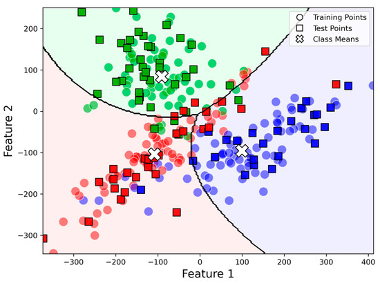
Figure 1. Decision boundaries of Gaussian naive Bayes for three classes, with green, red, and blue regions representing predicted class areas.

3. Proposed Methodology

This section presents two classifiers developed to enhance the traditional NB approach. Initially, we introduced randomized feature naive Bayes (RF-NB), a preliminary classifier intended to mitigate the restrictive assumption of conditional feature independence by incorporating randomized feature selection. Subsequently, building upon RF-NB, we propose the randomized feature and bootstrap sampling naive Bayes (RFB-NB) as our ultimate classifier.

3.1. Data Partitioning and Randomized Feature Selection

Consider a dataset represented by

$$S=\left\{\left.\left(x_i,y_i\right)\right|i=1,2,\mathrm{\dots },n\right\},$$

(15)

where each $x_i=(x_{i1},x_{i2},\mathrm{\dots },x_{id})\in {ℝ}^d$ is a feature vector of dimensionality $d$ and $y_i\in \left\{1,2,\mathrm{\dots },K\right\}$ denotes the corresponding class label. The dataset is randomly partitioned into a training set $S_{tr}$ and a test set $S_{te}$:

$$S_{tr}=\left\{\left.\left(x_i,y_i\right)\right|i=1,2,\mathrm{\dots },n_{tr}\right\},\hspace{1em}{S}_{te}=\left\{\left.\left(x_i,y_i\right)\right|i=n_{tr}+1,n_{tr}+2,\mathrm{\dots },n\right\}.$$

(16)

For each iteration $t$ of the proposed RFB-NB process, a random subset of features is selected. Let $m$ denote the number of selected features, where $m<d$. The indices of selected features are represented as

$$F_t\subset \left\{1,2,\mathrm{\dots },d\right\}, \mathrm{where} \left|F_t\right|=m.$$

(17)

This random feature selection introduces diversity at each iteration, mitigating feature dependency and enhancing robustness.

3.2. Bootstrap Sample Generation for Training

To further enhance model stability, bootstrap resampling is applied exclusively to the training set $S_{tr}$. For each iteration $t$, a bootstrap sample $S_t$ of size $n_{tr}$ is generated by sampling with a replacement from the original training set:

$$S_t=\left\{\left.\left(x_j,y_j\right)\right|j\in B_t,\hspace{1em}{B}_t~\mathrm{Multinomial}\left(n_{tr},{\displaystyle \frac{1}{n_{tr}}}\right)\right\}.$$

(18)

3.3. Gaussian Naive Bayes Training

For each iteration $t$, a Gaussian naive Bayes (GNB) classifier is trained using the bootstrap sample $S_t$ and selected feature subset $F_t$. Given class $Y=y_k$, the likelihood for each selected feature $X_j$, following a Gaussian distribution (as introduced in Section 2.1), is computed as

$$P(X_i|Y=y_k)={\displaystyle \frac{1}{\sqrt{2\pi {\sigma }_{jk}^2}}}\exp \left({\displaystyle \frac{-{\left(X_j-{\mu }_{ik}\right)}^2}{2{\sigma }_{jk}^2}}\right),$$

(19)

where the parameters ${\mu }_{jk}$ and ${\sigma }_{jk}^2$ are estimated from the training data according to (7).

3.4. Classification and Prediction Aggregation

After training, the Gaussian naive Bayes model is applied to classify instances in the test set $S_{te}$. For each test instance $x$, the posterior probability of class $y_k$ is computed as

$$P(Y=y_k|x)\propto \left({\displaystyle \frac{N_k}{N_{\mathrm{tr}}}}\right){\displaystyle \prod _{j\in F_t}\frac{1}{\sqrt{2\pi {\sigma }_{jk}^2}}\exp \left(\frac{-{\left(X_j-{\mu }_{ik}\right)}^2}{2{\sigma }_{jk}^2}\right)}.$$

(20)

The predicted class for iteration $t$ is determined by the maximum a posteriori estimate:

$${\widehat{y}}_t=\arg \underset{y_k}{\max }P\left(Y=y_k|x\right).$$

(21)

The final prediction, after running the classifier over $T$ iterations, is decided through majority voting:

$${\widehat{y}}_t=\arg \underset{y_k}{\max }{\displaystyle \sum _{t=1}^{T}I\left({\widehat{y}}_t=y_k\right)},$$

(22)

where $I\left(\cdot \right)$ is the indicator function.

3.5. Variance Reduction in RFB-NB

The predictive variance of the RFB-NB ensemble is reduced by averaging multiple independently trained classifiers. Formally, the variance for an ensemble classifier $f_{\mathrm{RFB}-\mathrm{NB}}(X)$ derived from $B$ classifiers, each trained on a bootstrap sample with randomly selected features, can be expressed as

$$Va{r}_D\left(f_{\mathrm{RFB}-\mathrm{NB}}(X)\right)={\displaystyle \frac{1}{B}}Va{r}_D\left(f_b(X)\right)+{\displaystyle \frac{B-1}{B}}Co{v}_D\left(f_b(X),f_{b^{\prime }}(X)\right),$$

(23)

where $Va{r}_D\left(\cdot \right)$ and $Co{v}_D\left(\cdot ,\cdot \right)$ denote the variance and covariance with respect to randomness introduced by bootstrap samples and feature subsets. The randomized selection of both data points and feature subsets ensures lower covariance between predictions of individual classifiers. Consequently, this approach effectively decreases overall ensemble variance, enhancing predictive stability and robustness, particularly beneficial for noisy or high-dimensional datasets.

3.6. Cross-Validation and Model Assessment

To objectively assess generalization capability and robustness, we employed 10-fold cross-validation. The complete dataset is systematically partitioned into ten mutually exclusive subsets (folds) of roughly equal size. Iteratively, each fold is treated as the validation set exactly once, with the remaining nine folds combined as the training set.

In each iteration, the RFB-NB classifier is trained according to the methodology described in Section 3.1, Section 3.2, Section 3.3 and Section 3.4 exclusively using the training subsets. The trained classifier is then assessed on the withheld validation subset. This process is repeated until every fold has served as the validation set exactly once. The predictive performance is evaluated through two primary metrics, namely accuracy and the weighted-average F1-score. The weighted-average F1-score is particularly useful as it accounts for potential class imbalance by computing the harmonic mean of precision and recall, weighted by class support. Formally, the weighted-average F1-score $({\mathrm{F}1}_{\mathrm{weighted}})$ is calculated as

$${\mathrm{F}1}_{\mathrm{weighted}}={\displaystyle {\sum }_{c=1}^C\frac{n_c}{N}}\cdot {\displaystyle \frac{2\cdot {\mathrm{Precision}}_c\cdot {\mathrm{Recall}}_c}{{\mathrm{Precision}}_c{+\mathrm{Recall}}_c}},$$

(24)

where $C$ is the total number of classes, $n_c$ represents the number of samples in class $c,$ $N$ is the total number of samples, and ${\mathrm{Precision}}_c$ and ${\mathrm{Recall}}_c$ denote precision and recall for class $c$, respectively.

Consequently, the final reported accuracy and weighted-average F1-score represent the average metrics computed across the ten validation iterations, providing reliable and unbiased estimates of predictive performance on unseen data. Formally, the 10-fold cross-validation accuracy ${(\mathrm{ACC}}_{CV})$ and weighted-average F1-score $({\mathrm{F}1}_{CV})$ are calculated as

$${\mathrm{ACC}}_{CV}={\displaystyle \frac{1}{10}}{\displaystyle \sum _{i=1}^{10}{\mathrm{ACC}}_i} \mathrm{and} {\mathrm{F}1}_{CV}={\displaystyle \frac{1}{10}}{\displaystyle \sum _{i=1}^{10}{\mathrm{F}1}_{\mathrm{weighted},\mathrm{i}}},$$

(25)

where ${\mathrm{ACC}}_i$ and ${\mathrm{F}1}_{\mathrm{weighted},\mathrm{i}}$ denote the accuracy and weighted-average F1-score obtained on the i-th validation fold, respectively.

3.7. Comparison of RFB-NB with TAN, WNB, and RF

It is important to acknowledge that the individual components of our proposed approaches—randomized feature selection and bootstrap aggregation—are established techniques widely used in ensemble learning frameworks. However, the novelty and contribution of the RF-NB and RFB-NB classifiers lie specifically in their integration of these ensemble strategies within the naive Bayes framework, which traditionally does not exploit such techniques. Unlike TAN [25], which explicitly models feature dependencies through a Bayesian network [26,27], or WNB, which assigns fixed feature weights, our methods implicitly handle feature interactions through randomization without additional structural complexity. Moreover, while inspired by random forests, our proposed methods maintain the probabilistic interpretable nature of NB rather than relying on decision trees, thus providing a distinct trade-off—an ensemble-enhanced naive Bayes classifier that achieves improved robustness and stability without sacrificing interpretability and computational simplicity.

4. Datasets

To evaluate the performance of the proposed RF-NB and RFB-NB models, we employed 20 publicly available datasets from diverse domains. These datasets vary in size, dimensionality, and response variable characteristics, allowing us to assess the model’s robustness and generalization capabilities across different scenarios.

4.1. Dataset Description

The datasets used in this study were sourced from the UCI Machine Learning Repository and Kaggle, covering diverse domains including medical diagnostics, finance, marketing analytics, telecommunications, agriculture, environmental studies, and product quality assessment. They encompass datasets with diverse feature spaces, including moderate-dimensional (e.g., Breast Cancer Wisconsin, Ionosphere) and low-dimensional (e.g., Zoo, Rice) data, featuring response variables that range from binary classifications (e.g., disease diagnosis, churn prediction), multi-class classifications (e.g., animal classification, waveform patterns, car quality), to ordinal and continuous outcomes (e.g., wine quality scores, occupancy estimation, bike demand levels). This diverse selection ensured a rigorous and robust evaluation of the proposed methodology across multiple real-world scenarios (Table 1).

Table 1. An overview of these datasets.

Reference	Dataset	n	p	Response	Distribution Percentage (%)
[31]	Breast Cancer Wisconsin	569	30	Malignant/benign	37.2/62.8
[32]	Pima Indians Diabetes	768	8	Diabetic/non-diabetic	34.9/65.1
[33]	Heart Disease	270	13	Presence/absence of disease	44.4/55.6
[34]	Indian Liver Patients	583	10	Liver disease/no disease	28.5/71.5
[35]	Hepatitis C Patients	612	12	Blood donor/suspect blood donor/hepatitis C/fibrosis/cirrhosis	91.4/3.2/2.5/2.1/0.8
[36]	Heart Failure Clinical Records	299	12	Death/not death	32.1/67.9
[37]	Bank Marketing	45,211	16	Subscribed/not Subscribed	11.5/88.5
[38]	German Credit	1000	20	Good/bad credit	70/30
[39]	Telecom Churn Prediction	7043	21	Churn/no churn	53.7/46.3
[40]	Bike Sharing	17,389	13	Low-/medium-/high-demand bike days	34.5/35.6/29.9
[41]	Ionosphere	351	34	Good/bad radar return	64.1/35.9
[42]	Waveform Database Generator	5000	21	Class 1/2/3	33.2/32.9/33.9
[43]	Room Occupancy	10,129	18	Number of occupants (0 to 3)	81.2/4.5/7.4/6.9
[44]	Zoo	101	17	Animal class (7 categories)	40.5/19.8/5.0/12.8/4.0/ 8.0/9.9
[45]	QSAR Bioconcentration Classes	779	9	Bioaccumulation classes (1 to 3)	59.1/8.1/32.8
[46]	Secondary Mushroom	61,068	20	Edible/poisonous	44.5/55.5
[47]	Rice	3810	7	Cammeo/Osmancik	42.8/57.2
[48]	Seeds	210	7	Three different varieties of wheat: Kama, Rosa, and Canadian	33.7/32.7/33.6
[49]	White Wine Quality	4898	11	Score quality (3 to 9)	0.4/3.3/29.8/44.9/17.9/ 3.6/0.1
[50]	Car Evaluation	1728	6	Evaluation level (unacceptable, acceptable, good, very good)	22.2/4.0/70.0/3.8

4.2. Dataset Characteristics and Selection Rationale

The datasets were carefully selected to rigorously evaluate the proposed methodology across diverse real-world classification tasks. The primary criteria for selection included (i) variability in feature dimensionality, (ii) diversity of response variable types, and (iii) representation of distinct practical domains. The chosen datasets were categorized into the following comprehensive groups, each encompassing multiple datasets:

(1)

Healthcare and Medical Diagnostics

These datasets involve predicting health-related outcomes using clinical and physiological attributes.

• Breast Cancer Wisconsin [31]: Binary classification (malignant vs. benign tumors).
• Pima Indians Diabetes [32]: Binary classification (presence or absence of diabetes).
• Heart Disease [33]: Binary classification predicting the presence or absence of heart disease based on clinical parameters.
• Indian Liver Patients [34]: Binary classification (liver disease prediction).
• Hepatitis C Patients [35]: Classification of blood donors and Hepatitis C patients based on laboratory and demographic values.
• Heart Failure Clinical Records [36]: Binary classification (survival vs. death outcomes).

(2)

Financial and Business Analytics

Datasets addressing customer behaviors, financial risks, and decision-making processes.

• Bank Marketing [37]: Predictive modeling of customer subscription behaviors.
• German Credit [38]: Binary classification of creditworthiness (good or bad credit).
• Telecom Churn Prediction [39]: Binary classification predicting customer churn behavior.
• Bike Sharing [40]: Ordinal classification predicting bike rental demand (categorized as low-, medium-, and high-demand days).

(3)

Signal Processing and Sensor-Based Classification

Datasets involving an analysis of signals or sensor measurements for classification tasks.

• Ionosphere [41]: Radar signal classification (good vs. bad signals).
• Waveform Database Generator [42]: Multi-class waveform pattern classification.
• Room Occupancy [43]: Prediction of room occupancy based on environmental sensors.

(4)

Biological and Environmental Classification

Datasets focused on classifying biological or agricultural samples and assessing environmental safety.

• Zoo [44]: Multi-class classification of animals into predefined categories.
• QSAR Bioconcentration Classes [45]: Classification of chemical compounds based on manually curated bioconcentration factors (BCF, fish) for QSAR modeling.
• Secondary Mushroom [46]: Binary classification (edible vs. poisonous mushrooms).
• Rice [47]: Binary classification identifying rice varieties (Cammeo vs. Osmancik).
• Seeds [48]: Multi-class classification of wheat kernel varieties based on geometrical and morphological features obtained using X-ray imaging techniques.

(5)

Product Quality Assessment

Datasets evaluating the quality or condition of consumer products.

• White Wine Quality [49]: Ordinal classification of wine quality scores (0–10).
• Car Evaluation [50]: Multi-class classification evaluating car quality (e.g., unacc, acc, good, very good).

4.3. Baseline Classification Methods

This section presents the baseline classification methods utilized for performance comparison, specifically random forest (RF) and k-nearest neighbors (KNN), outlining their theoretical foundations and practical implementations. These methods serve as benchmarks to evaluate the effectiveness and robustness of the proposed RFB-NB model.

(1)

Random Forest

Random forest is a prominent ensemble learning algorithm that constructs multiple decision trees during the training phase and merges their outputs to achieve improved prediction accuracy and control overfitting. Each decision tree is generated from bootstrapped samples of the training dataset, employing random subsets of features at each split. The final class prediction is made by aggregating the outputs through majority voting in classification tasks [51,52,53]. Formally, the classification prediction $\widehat{y}$ of RF for a given instance $x$ is defined as

$$\widehat{y}=\arg \underset{y\in Y}{\max }{\displaystyle \sum _{t=1}^{T}I\left(h_t(x)=y\right)},$$

(26)

where $h_t(x)$ denotes the prediction of the $t$-th decision tree and $T$ is the total number of decision trees. The RF classifier inherently accommodates non-linear relationships and interaction effects among features, demonstrating robustness and flexibility across diverse classification problems [54].

(2)

K-Nearest Neighbors

K-nearest neighbors is a simple yet effective non-parametric instance-based learning algorithm, widely used in classification tasks due to its conceptual simplicity and intuitive decision-making process [55,56,57]. Given an unknown instance, KNN classifies it by identifying its $K$ closest points from the training dataset based on a defined distance metric, typically Euclidean distance:

$$d(x,x_i)=\sqrt{{\displaystyle {\sum }_{j=1}^d{\left(x_j-x_{ij}\right)}^2}},$$

(27)

where $d$ represents the dimensionality of the feature space, $x$ is the instance to classify, and $x_i$ is a training instance. The predicted class label $\widehat{y}$ is obtained by majority voting among the $K$-nearest neighbors:

$$\widehat{y}=\arg \underset{y\in Y}{\max }{\displaystyle {\sum }_{x_i\in N_K(x)}I\left(y_i=y\right)},$$

(28)

where $N_K(x)$ denotes the set of the $K$-nearest neighbors to instance $x$ and $y_i$ is the class label of neighbor $x_i$. Despite its simplicity, KNN can effectively handle complex classification boundaries when properly tuned [58,59,60].

5. Results

5.1. Comparative Analysis by Domain

5.1.1. Healthcare and Medical Diagnostics

Performance results from the 10-fold cross-validation across healthcare datasets (summarized in Figure 2) indicate substantial improvements provided by RFB-NB and RF-NB methods over the classical NB, notably in the Heart Disease and Hepatitis C Patient datasets, where these methods consistently achieved higher median accuracies and weighted-average F1-scores. For the Pima Indians Diabetes dataset, both RFB-NB and RF-NB variants yielded superior median accuracy and F1-scores compared to RF and KNN methods, illustrating their robustness. Although RF exhibited notably higher median accuracy and F1-score in the Breast Cancer dataset, RFB-NB and RF-NB maintained higher minimum values, reflecting improved stability under varied conditions. In the Heart Failure Clinical Records dataset, RFB-NB delivered performance comparable to RF, significantly outperforming KNN. However, the Indian Liver Patient dataset posed challenges to all naive Bayes variants.

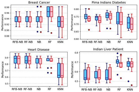
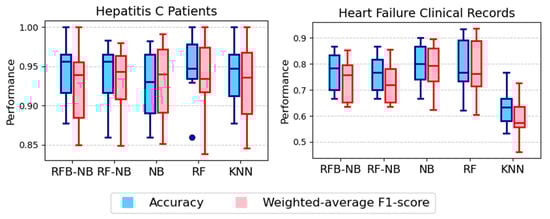
Figure 2. Accuracy distributions across healthcare and medical diagnostics datasets.

5.1.2. Financial and Business Analytics

Performance evaluations from 10-fold cross-validation across financial and business analytics datasets (summarized in Figure 3) highlight distinct predictive capabilities of RFB-NB and RF-NB relative to benchmark classifiers. For the Bank dataset, RF achieved the highest median accuracy and weighted-average F1-score, while RFB-NB and RF-NB notably outperformed classical NB, demonstrating enhanced predictive reliability. In the German Credit dataset, RF again exhibited superior median performance, with RFB-NB and RF-NB showing competitive accuracy and markedly better stability than KNN. The Telecom Churn dataset provided compelling evidence for RFB-NB’s superiority, as it delivered the highest median accuracy, closely followed by RF-NB, while all NB variants and KNN notably surpassed RF in weighted-average F1-scores. Finally, in the Bike Sharing dataset, the performance among RFB-NB, RF-NB, classical NB, and RF was closely aligned, consistently outperforming KNN.

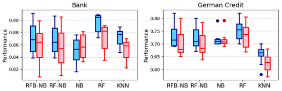
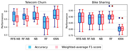
Figure 3. Accuracy distributions for financial and business analytics datasets.

5.1.3. Signal Processing and Sensor-Based Classification

Figure 4 presents the performance distributions for the signal processing and sensor-based datasets. In the Ionosphere dataset, RFB-NB consistently delivered a high accuracy and F1-score, outperforming KNN, RF-NB, and NB but still performing below RF. For the Waveform dataset, RF achieved the highest accuracy, while the NB variants struggled with this dataset and showed similar performance levels. In the Room Occupancy dataset, although KNN achieved the highest accuracy, RFB-NB and the NB variants exhibited higher median values for both metrics compared to RF.

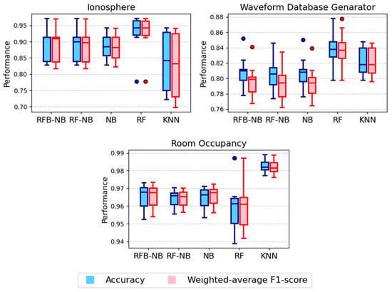
Figure 4. Accuracy distributions for signal processing and sensor-based classification datasets.

5.1.4. Biological and Environmental Classification

Accuracy and F1-score distributions for biological and environmental datasets are presented in Figure 5. In the Zoo dataset, RFB-NB achieved the highest median accuracy with exceptionally low variability, outperforming RF, RF-NB, classical NB, and especially KNN, which showed lower accuracy and greater variability. For the QSAR Bioconcentration dataset, RFB-NB again delivered higher median accuracy than classical NB and KNN and was comparable to RF; however, its F1-score was noticeably lower due to severe class imbalance. In the Secondary Mushroom dataset, both RFB-NB and RF-NB demonstrated stable and high accuracy, clearly outperforming the more variable performance of classical NB, RF, and KNN. Interestingly, classical NB yielded the highest F1-score, again highlighting the impact of class imbalance. For the Rice dataset, RF showed slightly higher median accuracy than RFB-NB, though RFB-NB and its variants still outperformed classical NB and KNN. Finally, in the Seeds dataset, RFB-NB achieved the highest median accuracy and F1-score, slightly outperforming the other classifiers. In this case, the alignment between accuracy and F1-score reflects the more balanced class distribution.

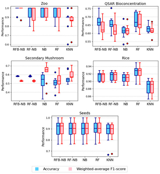
Figure 5. Accuracy distributions for biological and environmental classification datasets.

5.1.5. Product Quality Assessment

Figure 6 shows the accuracy and F1-score distributions for product quality assessment datasets. In the White Wine Quality dataset, RF achieved the highest accuracy and F1-score, followed by KNN and RFB-NB, both of which outperformed classical NB. In terms of F1-score, all methods appeared comparable except for NB, which showed notably poor performance. For the Car Evaluation dataset, KNN attained the highest median performance for both metrics. Among the naive Bayes variants, RFB-NB had the highest median accuracy but a relatively low F1-score. Overall, while RF and KNN dominated in this domain, RFB-NB remained the most competitive among the NB-based methods.

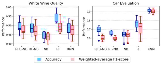
Figure 6. Accuracy distributions for product quality assessment datasets.

5.2. Stability and Robustness Evaluation

Although the stability of RFB-NB varies across datasets, certain cases clearly highlight its advantages. For instance, Figure 2 (Breast Cancer dataset) and Figure 5 (Secondary Mushroom and Rice) demonstrate narrower performance ranges for RFB-NB compared to RF and KNN, indicating improved prediction stability. Similarly, in Figure 3 (Telecom Churn) and Figure 4 (Room Occupancy), RFB-NB exhibits relatively tighter boxplots than RF. However, for datasets such as Hepatitis C Patients (Figure 2) and German Credit (Figure 3), the performance variability between RFB-NB and other classifiers like RF and KNN is comparable, suggesting no substantial robustness advantage. Thus, while RFB-NB generally achieves robust predictive performance, the extent of its stability benefits noticeably depends on specific dataset characteristics.

5.3. Overall Comparative Performance

Table 2 rigorously summarizes classifier performance across all twenty datasets, including statistical significance tests using Friedman and Wilcoxon signed-rank analyses. The RF classifier consistently achieved the highest mean accuracy across most datasets; however, only 5 out of the 20 datasets (Breast Cancer Wisconsin, Indian Liver Patients, Ionosphere, Room Occupancy, and Car Evaluation) showed statistically significant superiority over RFB-NB.

Table 2. Dataset-level comparative performance with Friedman test statistics and significant Wilcoxon signed-rank comparisons across 20 datasets.

Dataset	Top Accuracy (Mean)	Top Accuracy (Mean)	Friedman p-Value	Significant Wilcoxon Post Hoc (vs. RFB-NB)
Breast Cancer Wisconsin	RF (0.958)	RF (0.957)	0.0319	RF better (p = 0.0494)
Pima Indians Diabetes	RFB-NB (0.753)	NB (0.748)	0.0357	RFB-NB better than KNN (p = 0.0199)
Heart Disease	RFB-NB (0.848)	RFB-NB (0.847)	<0.0001	RFB-NB better than KNN
Indian Liver Patients	RF (0.701)	RF (0.677)	<0.0001	RF (p = 0.0020), KNN (p = 0.0078) better than RFB-NB
Hepatitis C Patients	RF (0.947)	RF (0.938)	0.2842	None
Heart Failure Clinical Records	NB (0.796)	NB (0.784)	0.0005	RFB-NB better than KNN (p = 0.0076)
Bank Marketing	RF (0.896)	RF (0.872)	<0.0001	RF better (p = 0.0039), RFB-NB better than NB (p = 0.0098)
German Credit	RF (0.751)	RF (0.732)	0.0001	RFB-NB better than KNN (p = 0.0020)
Telecom Churn Prediction	NB (0.550)	NB (0.538)	0.1644	None
Bike Sharing	RF (0.906)	RF (0.906)	0.0001	RFB-NB better than KNN (p = 0.0076)
Ionosphere	RF (0.929)	RF (0.928)	0.0004	RF better (p = 0.0391), RFB-NB better than KNN (p = 0.0117)
Waveform Database Generator	RF (0.841)	RF (0.840)	0.0002	RF better (p = 0.0020)
Room Occupancy	KNN (0.997)	KNN (0.997)	<0.0001	RF (p = 0.0420), KNN (p = 0.0020) better than RFB-NB
Zoo	RFB-NB (0.960)	RFB-NB (0.961)	0.1518	None
QSAR Bioconcentration Classes	RF (0.680)	RF (0.665)	0.0003	RFB-NB better than NB (p = 0.0020) and RF-NB (p = 0.0176)
Secondary Mushroom	RFB-NB (0.583)	NB (0.628)	0.0114	RFB-NB better than RF (p = 0.0117)
Rice	RF (0.924)	RF (0.924)	<0.0001	RFB-NB better than KNN (p = 0.0020)
Seeds	RF (0.909)	RF (0.909)	0.1749	None
White Wine Quality	RF (0.541)	RF (0.491)	<0.0001	RFB-NB better than NB and RF-NB (p = 0.0020, 0.0215), RF better (p = 0.0020)
Car Evaluation	KNN (0.915)	KNN (0.905)	<0.0001	KNN, RF, and NB better than RFB-NB (p = 0.0020, 0.0059, 0.0059)

Note: Datasets indicated in bold denote cases where the RFB-NB classifier significantly outperformed at least one competing classifier (Wilcoxon signed-rank test, p < 0.05).

The proposed RFB-NB method demonstrated statistically significant improvements (α = 0.05) over at least one competing classifier in multiple datasets, specifically those highlighted in bold in Table 2, namely Pima Indians Diabetes, Heart Disease, Heart Failure Clinical Records, Bank Marketing, German Credit, Bike Sharing, Ionosphere, QSAR Bioconcentration Classes, Secondary Mushroom, Rice, and White Wine Quality. These significant outcomes underscore RFB-NB’s strong capabilities, confirming its practical utility and effectiveness as a competitive alternative to existing classifiers.

The aggregated results shown in Table 3 further validate the strong overall performance of RF (mean accuracy = 0.8061; average rank = 1.875), with RFB-NB closely following (mean accuracy = 0.7869; average rank = 2.375) and notably displaying the lowest mean variability (0.0447), emphasizing its stability across datasets.

Table 3. Aggregate comparative results of classification accuracy across 20 datasets.

Model	Mean Accuracy	Mean Std. Dev.	Average Rank
RF	0.8061	0.0591	1.875
RFB-NB	0.7869	0.0447	2.375
RF-NB	0.7798	0.0449	3.000
NB	0.7672	0.0573	3.775
KNN	0.7494	0.0523	3.975

Furthermore, Table 4 summarizes the weighted-average F1-score across the datasets, corroborating RF’s strong performance (mean F1-score = 0.7979; average rank = 2.025). RFB-NB maintained its competitive position, achieving the second highest mean F1-score (0.7841) and the lowest variability (0.0471), reinforcing its reliability and balanced performance.

Table 4. Aggregate comparative results of classification weighted-average F1-score across 20 datasets.

Model	Mean Accuracy	Mean Std. Dev.	Average Rank
RF	0.7979	0.0619	2.025
RFB-NB	0.7841	0.0471	2.600
NB	0.7758	0.0575	2.925
RF-NB	0.7726	0.0475	3.100
KNN	0.7579	0.0551	4.350

6. Conclusions

This study introduced two extensions of the classical NB classifier—RF-NB and RFB-NB—designed explicitly to address limitations inherent to NB through randomized feature selection and bootstrap aggregation. Extensive empirical evaluations across twenty diverse real-world datasets in medical diagnostics, financial analytics, sensor-based monitoring, biological classification, and product quality assessment illustrated the effectiveness of these methods. While RFB-NB consistently outperformed classical NB, RF-NB, and KNN in several scenarios, RF exhibited slightly higher average accuracy overall. Nevertheless, RFB-NB demonstrated distinct advantages by providing comparable accuracy alongside significantly reduced variance and improved stability. These benefits were particularly pronounced in challenging scenarios, notably datasets affected by considerable noise, high-dimensional feature spaces, or pronounced class imbalance (e.g., Breast Cancer and Telecom Churn datasets).

Statistical significance analyses using Friedman and Wilcoxon post-hoc tests further confirmed that RFB-NB significantly surpassed at least one benchmark method in 11 of the 20 datasets evaluated. These results emphasize that, despite RF’s superior accuracy in some scenarios, RFB-NB offers valuable complementary strengths—robustness and stability—making it an ideal choice for applications where interpretability, reliability, and computational efficiency are essential.

Future research should focus on exploring adaptive parameter tuning strategies, assessing RFB-NB’s performance in regression, multi-label classification, or further imbalanced scenarios, and conducting deeper theoretical investigations to precisely determine the optimal conditions under which RFB-NB delivers its greatest advantages.

References

- Huang, Y.; Li, W.; Macheret, F.; Gabriel, R.A.; Ohno-Machado, L. A Tutorial on Calibration Measurements and Calibration Models for Clinical Prediction Models. J. Am. Med. Inform. Assoc. 2020, 27, 621–633. [Google Scholar] [CrossRef]
- Wang, Q.; Garrity, G.M.; Tiedje, J.M.; Cole, J.R. Naive Bayesian Classifier for Rapid Assignment of rRNA Sequences into the New Bacterial Taxonomy. Appl. Environ. Microbiol. 2007, 73, 5261–5267. [Google Scholar] [CrossRef] [PubMed]
- Jurafsky, D.; Martin, J.H. Naive Bayes and Sentiment Classification. In Speech and Language Processing, 3rd ed.; Prentice Hall: Upper Saddle River, NJ, USA, 2019. [Google Scholar]
- Zhang, H. The Optimality of Naive Bayes. In Proceedings of the 17th International Florida Artificial Intelligence Research Society Conference, Menlo Park, CA, USA, 12–14 May 2004; pp. 562–567. [Google Scholar]
- Domingos, P.; Pazzani, M. On the Optimality of the Simple Bayesian Classifier under Zero-One Loss. Mach. Learn. 1997, 29, 103–130. [Google Scholar] [CrossRef]
- Rennie, J.D.M.; Shih, L.; Teevan, J.; Karger, D.R. Tackling the Poor Assumptions of Naive Bayes Text Classifiers. In Proceedings of the Twentieth International Conference on Machine Learning (ICML-2003), Washington, DC, USA, 21–24 August 2003; Available online: https://api.semanticscholar.org/CorpusID:13606541 (accessed on 10 December 2024).
- Rish, I. An Empirical Study of the Naive Bayes Classifier. In Proceedings of the IJCAI 2001 Workshop on Empirical Methods in Artificial Intelligence, Seattle, WA, USA, 4 August 2001; pp. 41–46. [Google Scholar]
- Ratanamahatana, C.A.; Gunopulos, D. Feature Selection for the Naive Bayesian Classifier Using Decision Trees. Appl. Artif. Intell. 2003, 17, 475–487. [Google Scholar] [CrossRef]
- Askari, A.; d’Aspremont, A.; El Ghaoui, L. Naive Feature Selection: Sparsity in Naive Bayes. In Proceedings of the 23rd International Conference on Artificial Intelligence and Statistics, Online, 26–28 August 2020. [Google Scholar]
- Kohavi, R.; John, G.H. Wrappers for Feature Subset Selection. Artif. Intell. 1997, 97, 273–324. [Google Scholar] [CrossRef]
- Jiang, L.; Zhang, H.; Cai, Z.; Su, J. Learning Tree Augmented Naive Bayes for Ranking. In Proceedings of the 10th International Conference on Database Systems for Advanced Applications, Beijing, China, 17–20 April 2005; Lecture Notes in Computer Science; Springer: Berlin/Heidelberg, Germany, 2005; Volume 3453, pp. 688–698. [Google Scholar] [CrossRef]
- Hall, M.A. Correlation-Based Feature Selection for Machine Learning. Ph.D. Thesis, University of Waikato, Hamilton, New Zealand, 1999. [Google Scholar]
- May, S.S.; Isafiade, O.E.; Ajayi, O.O. An Enhanced Naïve Bayes Model for Crime Prediction Using Recursive Feature Elimination. In Proceedings of the 2021 Conference on Information Communications Technology and Society (ICTAS), Durban, South Africa, 10–11 March 2021. [Google Scholar]
- Pujianto, U.; Wibowo, A.; Widhiastuti, R.; Asma, D.A.I. Comparison of Naive Bayes and Random Forests Classifier in the Classification of News Article Popularity as Learning Material. J. Phys. Conf. Ser. 2021, 1808, 012028. [Google Scholar] [CrossRef]
- Aridas, C.K.; Kotsiantis, S.B.; Vrahatis, M.N. Increasing Diversity in Random Forests Using Naive Bayes. In Machine Learning and Knowledge Discovery in Databases; Springer: Cham, Switzerland, 2016; pp. 75–86. [Google Scholar] [CrossRef]
- Efron, B.; Tibshirani, R.J. An Introduction to the Bootstrap; Chapman and Hall/CRC: Boca Raton, FL, USA, 1994. [Google Scholar]
- Breiman, L. Random Forests. Mach. Learn. 2001, 45, 5–32. [Google Scholar] [CrossRef]
- Friedman, J.; Hastie, T.; Tibshirani, R. The Elements of Statistical Learning, 2nd ed.; Springer: New York, NY, USA, 2009. [Google Scholar]
- Liaw, A.; Wiener, M. Classification and Regression by randomForest. R News 2002, 2, 18–22. [Google Scholar]
- Zhang, H.; Sheng, S. Learning Weighted Naive Bayes with Accurate Ranking. In Proceedings of the 4th IEEE International Conference on Data Mining, Brighton, UK, 1–4 November 2004. [Google Scholar]
- Srisuradetchai, P.; Suksrikran, K. Random Kernel K-Nearest Neighbors Regression. Front. Big Data 2024, 7, 1402384. [Google Scholar] [CrossRef]
- Panichkitkosolkul, W.; Srisuradetchai, P. Bootstrap Confidence Intervals for the Parameter of Zero-Truncated Poisson-Ishita Distribution. Thail. Stat. 2022, 20, 918–927. Available online: https://ph02.tci-thaijo.org/index.php/thaistat/article/view/247474 (accessed on 10 January 2025).
- Jiang, L.; Zhang, H.; Cai, Z. A Novel Bayes Model: Hidden Naive Bayes. IEEE Trans. Knowl. Data Eng. 2009, 21, 1361–1371. [Google Scholar] [CrossRef]
- Guyon, I.; Elisseeff, A. An Introduction to Variable and Feature Selection. J. Mach. Learn. Res. 2003, 3, 1157–1182. [Google Scholar] [CrossRef][Green Version]
- Friedman, N.; Geiger, D.; Goldszmidt, M. Bayesian Network Classifiers. Mach. Learn. 1997, 29, 131–163. [Google Scholar] [CrossRef]
- Duan, W.; Lu, X. Weighted Naive Bayesian Classifier Model Based on Information Gain. In Proceedings of the 2010 International Conference on Intelligent System Design and Engineering Application, Changsha, China, 13–14 October 2010; pp. 819–822. [Google Scholar] [CrossRef]
- Foo, L.-K.; Chua, S.-L.; Ibrahim, N. Attribute Weighted Naïve Bayes Classifier. Comput. Mater. Contin. 2021, 71, 1945–1957. [Google Scholar] [CrossRef]
- McCallum, A.; Nigam, K. A Comparison of Event Models for Naive Bayes Text Classification. In Proceedings of the AAAI Workshop on Learning for Text Categorization, Madison, WI, USA, 26–27 July 1998. [Google Scholar]
- John, G.H.; Langley, P. Estimating Continuous Distributions in Bayesian Classifiers. In Proceedings of the Eleventh Conference on Uncertainty in Artificial Intelligence, Montréal, QC, Canada, 18–20th August 1995; pp. 338–345. [Google Scholar]
- Murphy, K.P. Machine Learning: A Probabilistic Perspective; MIT Press: Cambridge, MA, USA, 2012. [Google Scholar]
- Wolberg, W.; Mangasarian, O.; Street, N.; Street, W. Breast Cancer Wisconsin (Diagnostic) [Dataset]. UCI Machine Learning Repository. 1995. Available online: https://archive.ics.uci.edu/dataset/17/breast+cancer+wisconsin+diagnostic (accessed on 15 January 2025).
- Smith, J.W.; Everhart, J.E.; Dickson, W.C.; Knowler, W.C.; Johannes, R.S. Using the ADAP Learning Algorithm to Forecast the Onset of Diabetes Mellitus. In Proceedings of the Annual Symposium on Computer Applications in Medical Care, Washington, DC, USA, 9–11 November 1988; pp. 261–265. Available online: https://www.ncbi.nlm.nih.gov/pmc/articles/PMC2245318/ (accessed on 15 January 2025).
- Dua, D.; Graff, C. Heart Disease Dataset [Dataset]. UCI Machine Learning Repository. 2019. Available online: https://archive.ics.uci.edu/dataset/145/statlog+heart (accessed on 15 January 2025).
- Ramana, B.; Venkateswarlu, N. Indian Liver Patient Dataset (ILPD) [Dataset]. UCI Machine Learning Repository. 2022. Available online: https://archive.ics.uci.edu/dataset/225/ilpd+indian+liver+patient+dataset (accessed on 15 January 2025).
- Lichtinghagen, R.; Klawonn, F.; Hoffmann, G. Hepatitis C Virus Data (HCV) [Dataset]. UCI Machine Learning Repository. 2020. Available online: https://archive.ics.uci.edu/dataset/571/hcv+data (accessed on 15 January 2025).
- Chicco, D.; Jurman, G. Heart Failure Clinical Records [Dataset]. UCI Machine Learning Repository. 2020. Available online: https://archive.ics.uci.edu/dataset/519/heart+failure+clinical+records (accessed on 15 January 2025).
- Moro, S.; Rita, P.; Cortez, P. Bank Marketing Dataset [Dataset]. UCI Machine Learning Repository. 2014. Available online: https://archive.ics.uci.edu/dataset/222/bank+marketing (accessed on 15 January 2025).
- Hofmann, H. German Credit Data [Dataset]. UCI Machine Learning Repository. 1994. Available online: https://archive.ics.uci.edu/dataset/144/statlog+german+credit+data (accessed on 15 January 2025).
- Berson, A.; Smith, S.; Thearling, K. Building Data Mining Applications for CRM; McGraw-Hill: New York, NY, USA, 2000. [Google Scholar]
- Fanaee-T, H. Bike Sharing Dataset [Dataset]. UCI Machine Learning Repository. 2013. Available online: https://archive.ics.uci.edu/dataset/275/bike+sharing+dataset (accessed on 15 January 2025).
- Sigillito, V.; Wing, S.; Hutton, L.; Baker, K. Ionosphere [Dataset]. UCI Machine Learning Repository. 1989. Available online: https://archive.ics.uci.edu/dataset/52/ionosphere (accessed on 15 January 2025).
- Breiman, L.; Stone, C. Waveform Database Generator (Version 1) [Dataset]. UCI Machine Learning Repository. 1984. Available online: https://archive.ics.uci.edu/dataset/107/waveform+database+generator+version+1 (accessed on 15 January 2025).
- Singh, A.P.; Jain, V.; Chaudhari, S.; Kraemer, F.A.; Werner, S.; Garg, V. Room Occupancy Estimation [Dataset]. UCI Machine Learning Repository. 2018. Available online: https://archive.ics.uci.edu/dataset/864/room+occupancy+estimation (accessed on 15 January 2025).
- Forsyth, R. Zoo [Dataset]. UCI Machine Learning Repository. 1990. Available online: https://archive.ics.uci.edu/dataset/111/zoo (accessed on 15 January 2025).
- UCI Machine Learning Repository. QSAR Bioconcentration Classes Dataset [Dataset]. 2019. Available online: https://archive.ics.uci.edu/dataset/510/qsar+bioconcentration+classes+dataset (accessed on 15 January 2025).
- Wagner, D.; Heider, D.; Hattab, G. Secondary Mushroom [Dataset]. UCI Machine Learning Repository. 2021. Available online: https://archive.ics.uci.edu/dataset/848/secondary+mushroom+dataset (accessed on 15 January 2025).
- Cınar, I.; Koklu, M. Rice (Cammeo and Osmancik) [Dataset]. UCI Machine Learning Repository. 2019. Available online: https://archive.ics.uci.edu/dataset/545/rice+cammeo+and+osmancik (accessed on 15 January 2025).
- Charytanowicz, M.; Niewczas, J.; Kulczycki, P.; Kowalski, P.; Lukasik, S. Seeds [Dataset]. UCI Machine Learning Repository. 2010. Available online: https://archive.ics.uci.edu/dataset/236/seeds (accessed on 15 January 2025).
- Cortez, P.; Cerdeira, A.; Almeida, F.; Matos, T.; Reis, J. Wine Quality [Dataset]. UCI Machine Learning Repository. 2009. Available online: https://archive.ics.uci.edu/dataset/186/wine+quality (accessed on 15 January 2025).
- Bohanec, M. Car Evaluation [Dataset]. UCI Machine Learning Repository. 1988. Available online: https://archive.ics.uci.edu/dataset/19/car+evaluation (accessed on 15 January 2025).
- Vergni, L.; Todisco, F. A Random Forest Machine Learning Approach for the Identification and Quantification of Erosive Events. Water 2023, 15, 2225. [Google Scholar] [CrossRef]
- Svoboda, J.; Štych, P.; Laštovička, J.; Paluba, D.; Kobliuk, N. Random Forest Classification of Land Use, Land-Use Change and Forestry (LULUCF) Using Sentinel-2 Data—A Case Study of Czechia. Remote Sens. 2022, 14, 1189. [Google Scholar] [CrossRef]
- Purwanto, A.D.; Wikantika, K.; Deliar, A.; Darmawan, S. Decision Tree and Random Forest Classification Algorithms for Mangrove Forest Mapping in Sembilang National Park, Indonesia. Remote Sens. 2023, 15, 16. [Google Scholar] [CrossRef]
- Tian, S.; Zhang, X.; Tian, J.; Sun, Q. Random Forest Classification of Wetland Landcovers from Multi-Sensor Data in the Arid Region of Xinjiang, China. Remote Sens. 2016, 8, 954. [Google Scholar] [CrossRef]
- Kamlangdee, P.; Srisuradetchai, P. Circular Bootstrap on Residuals for Interval Forecasting in K-NN Regression: A Case Study on Durian Exports. Sci. Technol. Asia 2025, 30, 79–94. Available online: https://ph02.tci-thaijo.org/index.php/SciTechAsia/article/view/255306 (accessed on 28 March 2025).
- Srisuradetchai, P.; Panichkitkosolkul, W. Using Ensemble Machine Learning Methods to Forecast Particulate Matter (PM2.5) in Bangkok, Thailand. In Multi-Disciplinary Trends in Artificial Intelligence; Surinta, O., Kam, F., Yuen, K., Eds.; Lecture Notes in Computer Science; Springer: Cham, Switzerland, 2022; Volume 13651. [Google Scholar] [CrossRef]
- Srisuradetchai, P. A Novel Interval Forecast for K-Nearest Neighbor Time Series: A Case Study of Durian Export in Thailand. IEEE Access 2024, 12, 2032–2044. [Google Scholar] [CrossRef]
- Boateng, E.Y.; Otoo, J.; Abaye, D.A. Basic Tenets of Classification Algorithms K-Nearest-Neighbor, Support Vector Machine, Random Forest and Neural Network: A Review. J. Data Anal. Inf. Process. 2020, 8, 341–357. [Google Scholar] [CrossRef]
- Bellino, G.M.; Schiaffino, L.; Battisti, M.; Guerrero, J.; Rosado-Muñoz, A. Optimization of the KNN Supervised Classification Algorithm as a Support Tool for the Implantation of Deep Brain Stimulators in Patients with Parkinson’s Disease. Entropy 2019, 21, 346. [Google Scholar] [CrossRef] [PubMed]
- Florimbi, G.; Fabelo, H.; Torti, E.; Lazcano, R.; Madroñal, D.; Ortega, S.; Salvador, R.; Leporati, F.; Danese, G.; Báez-Quevedo, A.; et al. Accelerating the K-Nearest Neighbors Filtering Algorithm to Optimize the Real-Time Classification of Human Brain Tumor in Hyperspectral Images. Sensors 2018, 18, 2314. [Google Scholar] [CrossRef] [PubMed]
Disclaimer/Publisher’s Note: The statements, opinions and data contained in all publications are solely those of the individual author(s) and contributor(s) and not of MDPI and/or the editor(s). MDPI and/or the editor(s) disclaim responsibility for any injury to people or property resulting from any ideas, methods, instructions or products referred to in the content. |
© 2025 by the authors. Published by MDPI on behalf of the International Institute of Knowledge Innovation and Invention. Licensee MDPI, Basel, Switzerland. This article is an open access article distributed under the terms and conditions of the Creative Commons Attribution (CC BY) license (https://creativecommons.org/licenses/by/4.0/).