
Modeling Wildfire Spread with an Irregular Graph Network
 , ,
, ,
Abstract
:1. Introduction
2. Materials and Methods
2.1. Experimental Area
2.2. Variable-Scale Landscape with IGN
2.2.1. Definition of the IGN
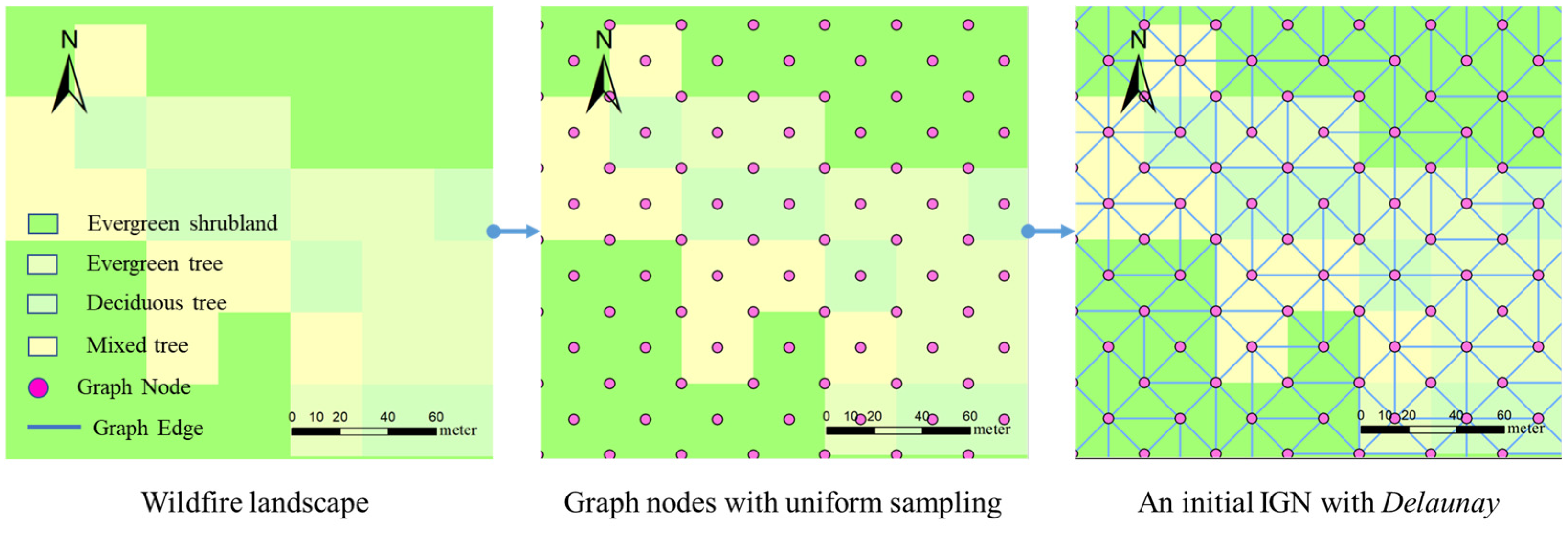
2.2.2. IGN Initialization
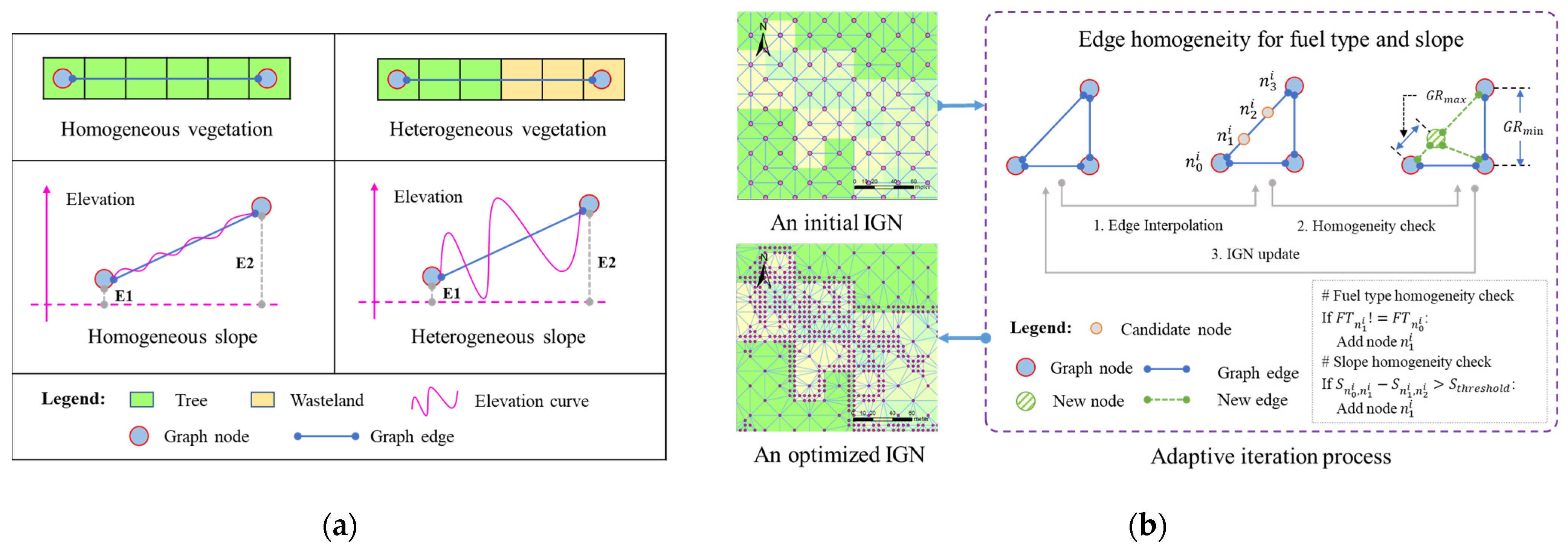
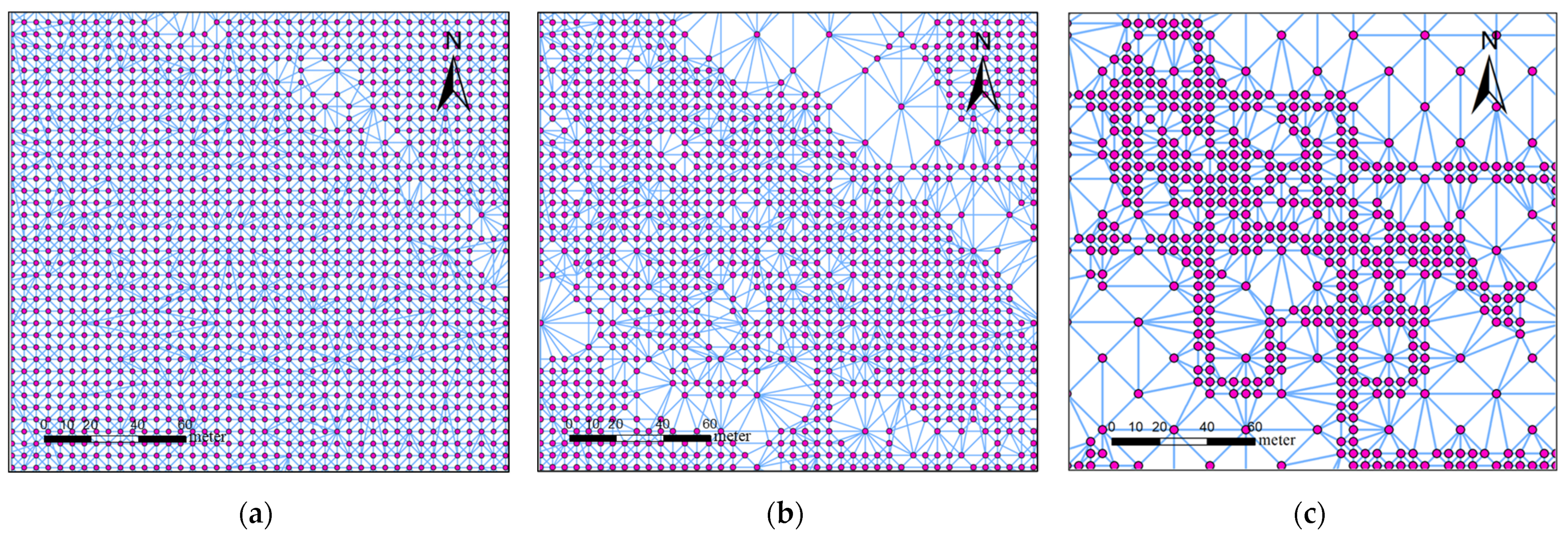
2.2.3. IGN Adaptive Optimization
2.3. Deep Learning-Based Spread Model
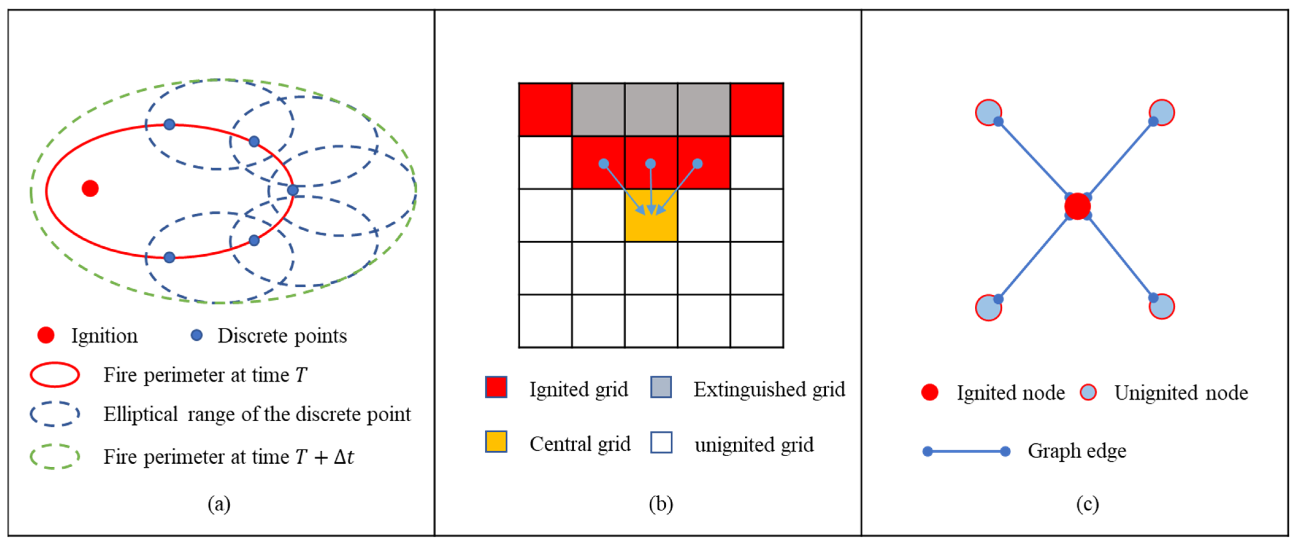
2.3.1. Definition of the IGN Spread
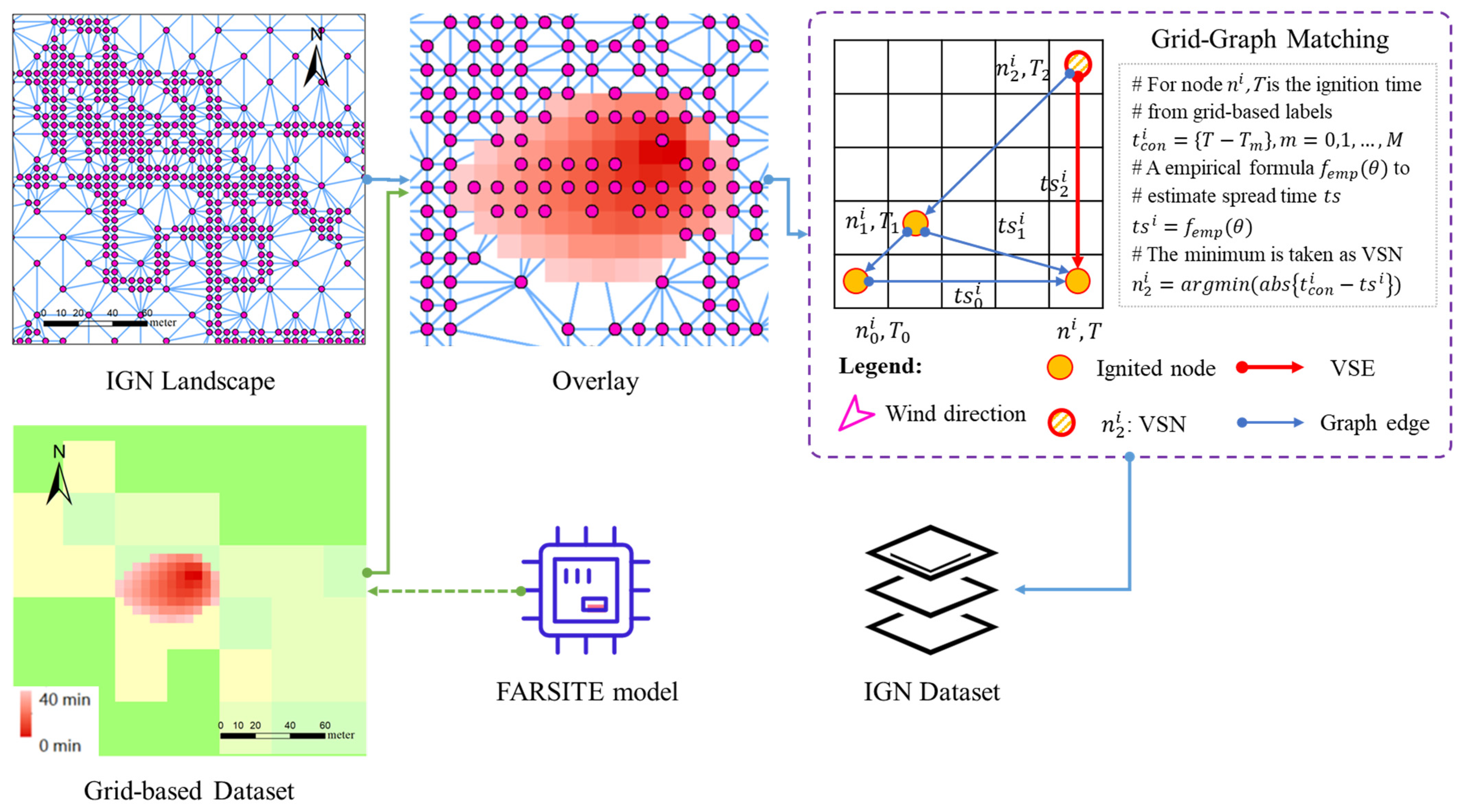
2.3.2. Construction of Grid-Based Dataset
2.3.3. Construction of IGN Dataset
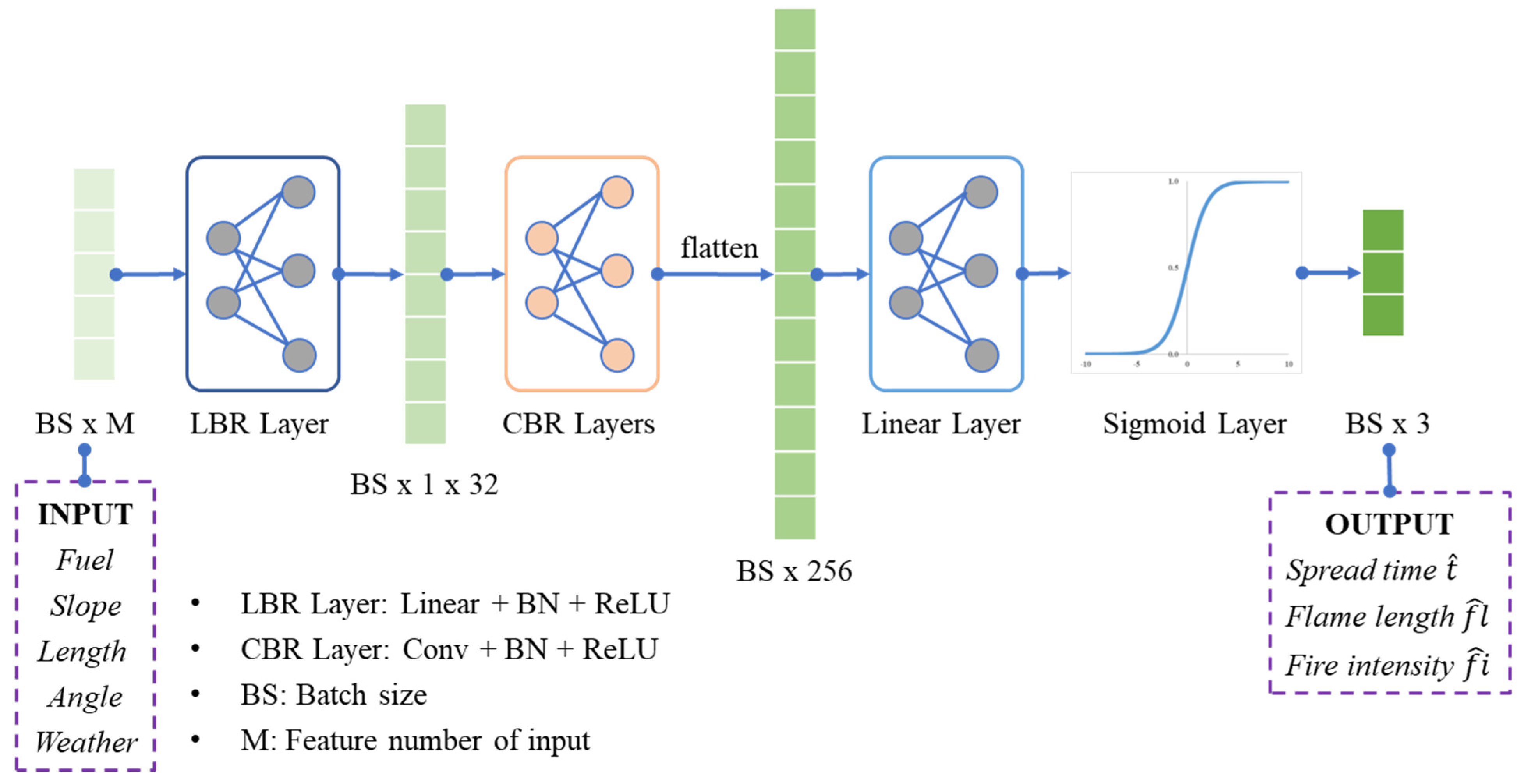
2.3.4. Design of Deep Neural Network
3. Results
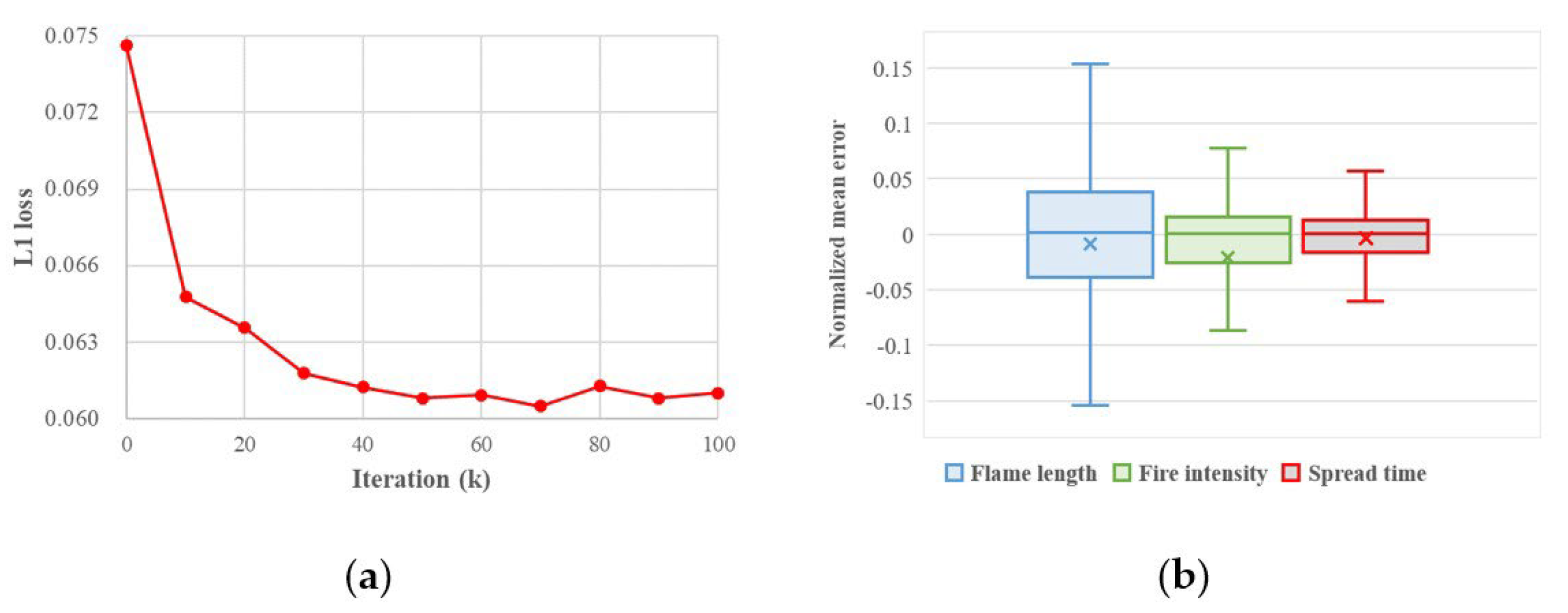
3.1. WFDNN Result
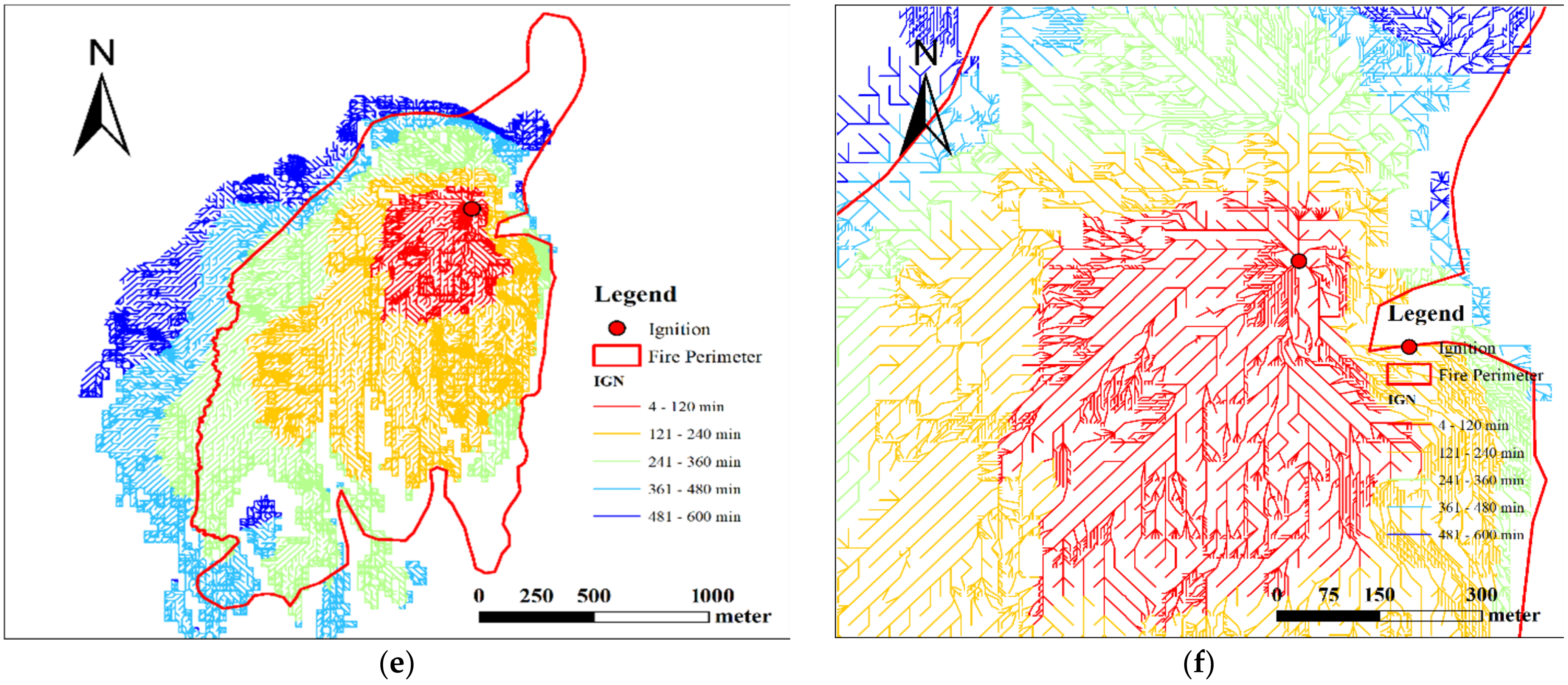
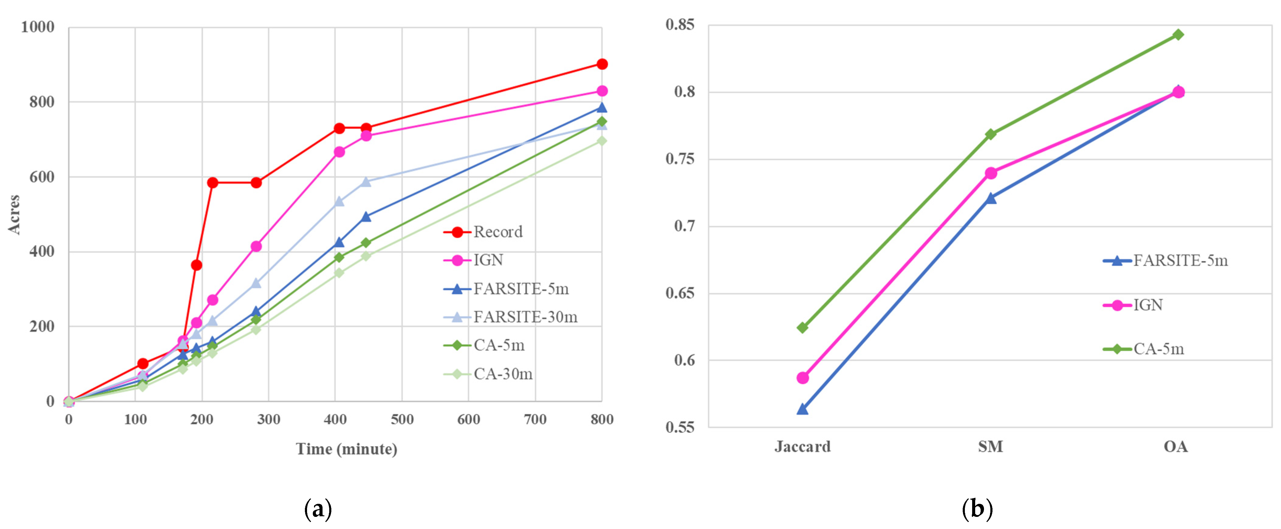
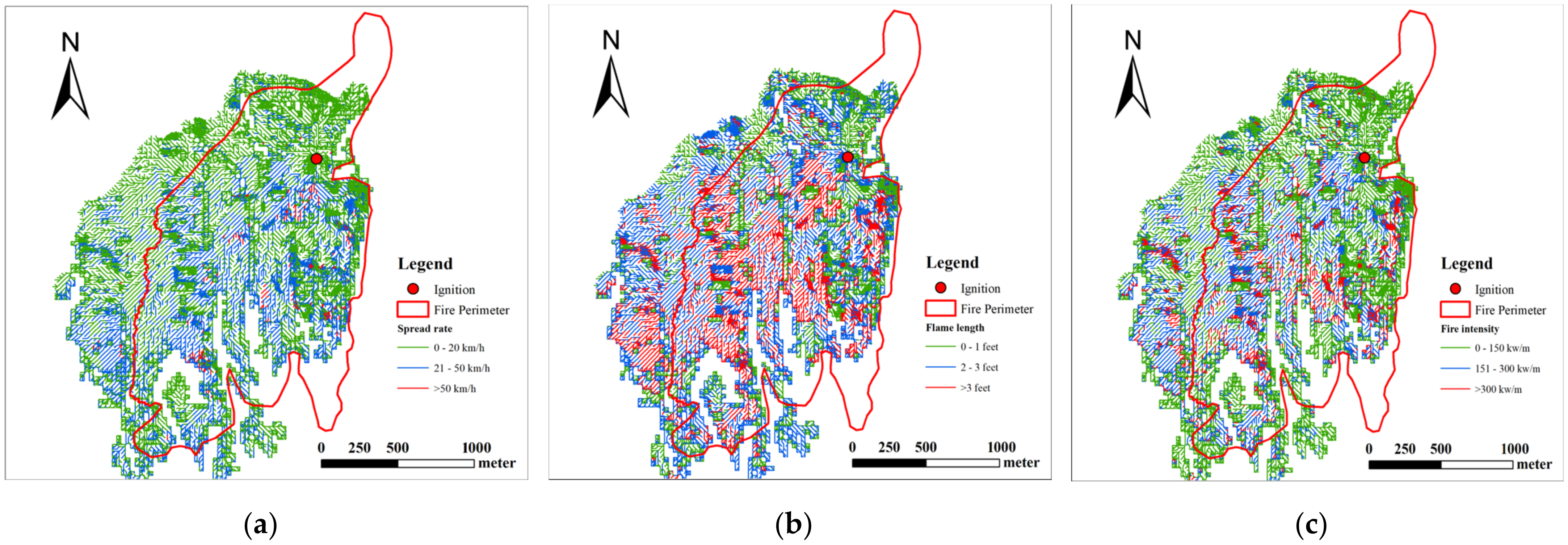
3.2. Results of Getty Fire Case
4. Discussion
4.1. Analysis of Getty Case
4.2. Effect of Elevation Difference Threshold on IGN
4.3. VSE Dataset Analysis
5. Conclusions
Author Contributions
Funding
Data Availability Statement
Conflicts of Interest
Appendix A

| FARSITE | CA | IGN | |
|---|---|---|---|
| Theoretical principle | Thermal physics | Thermal physics | Deep learning |
| Spread pattern | Huygens | Cellular automata | Graph network |
| Landscape type | Vector | Grid | Vector |
| Output format | Polygon or Grid | Grid | Graph |
- (1)
- Theoretical principle
- (2)
- Spread pattern
- (3)
- Landscape type
- (4)
- Output format

Appendix B
| Algorithm A1 Adaptive iteration process in IGN optimization. |
| , the initial IGN with uniform sampling and Delaunay algorithm , the optimized IGN is the edges of the graph network = null # To store newly inserted nodes Iter_counter = 0 # Count the time of iteration Iter_count_max = 1e3 # The maximum time of iteration # Adaptive iteration while True: # count the number of iteration Iter_counter += 1 : # Step 1: Edge interpolation. Use equally spaced interpolation to obtain a candidate node set ) # Candidate node set, containing M+1 nodes # Step 2: homogeneity check: fuel type and slope : # fuel type : , thus we add the node to avoid the heterogeneity. # Slope homogeneity. Here we use elevation difference to replace ) # Get elevation differences of neighboring nodes : # The elevation has a large wave, thus we add the node to eliminate it. # Step 3: Reconstruct the IGN by Delaunay algorithm, ) # Concatenate and generate new node set ) # Update the G with new nodes G # if no more new nodes or reaching the maximum iteration ) or Iter_counter> Iter_count_max: Break = G |
Appendix C
| Algorithm A2 Grid-Graph matching algorithm. |
| grid-based labels , graph-based labels ) is the number of graph nodes # Set VSEs = null = null # Search the VSE and VSN : # Get the spread time of each connected edge is the proprieties of graph edges # The minimum is taken as the VSE }) # j is the index of the node with the minimum difference # Add the VSE }) # Get the dataset = VSEs |
References
- Bowman, D.M.J.S.; Balch, J.K.; Artaxo, P.; Bond, W.J.; Carlson, J.M.; Cochrane, M.A.; D’Antonio, C.M.; DeFries, R.S.; Doyle, J.C.; Harrison, S.P.; et al. Fire in the Earth System. Science 2009, 324, 481–484. [Google Scholar] [CrossRef] [PubMed]
- Doerr, S.H.; Santín, C. Global trends in wildfire and its impacts: Perceptions versus realities in a changing world. Philos. Trans. R. Soc. B Biol. Sci. 2016, 371, 20150345. [Google Scholar] [CrossRef] [PubMed] [Green Version]
- Godfree, R.C.; Knerr, N.; Encinas-Viso, F.; Albrecht, D.; Bush, D.; Cargill, D.C.; Clements, M.; Gueidan, C.; Guja, L.K.; Harwood, T.; et al. Implications of the 2019–2020 megafires for the biogeography and conservation of Australian vegetation. Nat. Commun. 2021, 12, 1023. [Google Scholar] [CrossRef] [PubMed]
- Ball, G.; Regier, P.; González-Pinzón, R.; Reale, J.; Van Horn, D. Wildfires increasingly impact western US fluvial networks. Nat. Commun. 2021, 12, 2484. [Google Scholar] [CrossRef] [PubMed]
- Zou, Y.; Rasch, P.J.; Wang, H.; Xie, Z.; Zhang, R. Increasing large wildfires over the western United States linked to diminishing sea ice in the Arctic. Nat. Commun. 2021, 12, 6048. [Google Scholar] [CrossRef]
- Tang, W.; Llort, J.; Weis, J.; Perron, M.M.G.; Basart, S.; Li, Z.; Sathyendranath, S.; Jackson, T.; Rodriguez, E.S.; Proemse, B.C.; et al. Widespread phytoplankton blooms triggered by 2019–2020 Australian wildfires. Nature 2021, 597, 370–375. [Google Scholar] [CrossRef]
- Minas, J.P.; Hearne, J.W.; Handmer, J.W. A review of operations research methods applicable to wildfire management. Int. J. Wildland Fire 2012, 21, 189–196. [Google Scholar] [CrossRef] [Green Version]
- Page, W.G.; Freeborn, P.H.; Butler, B.W.; Jolly, W.M. A review of US wildland firefighter entrapments: Trends, important environmental factors and research needs. Int. J. Wildland Fire 2019, 28, 551–569. [Google Scholar] [CrossRef]
- Sullivan, A.L. Wildland surface fire spread modelling, 1990–2007. 2: Empirical and quasi-empirical models. Int. J. Wildland Fire 2009, 18, 369–386. [Google Scholar] [CrossRef] [Green Version]
- Sullivan, A.L. Wildland surface fire spread modelling, 1990–2007. 1: Physical and quasi-physical models. Int. J. Wildland Fire 2009, 18, 349–368. [Google Scholar] [CrossRef]
- Sullivan, A.L. Wildland surface fire spread modelling, 1990–2007. 3: Simulation and mathematical analogue models. Int. J. Wildland Fire 2009, 18, 387–403. [Google Scholar] [CrossRef] [Green Version]
- Sullivan, A.; Sharples, J.; Matthews, S.; Plucinski, M. A downslope fire spread correction factor based on landscape-scale fire behaviour. Environ. Model. Softw. 2014, 62, 153–163. [Google Scholar] [CrossRef]
- Fernandes, P.M.; Botelho, H.S.; Rego, F.C.; Loureiro, C. Empirical modelling of surface fire behaviour in maritime pine stands. Int. J. Wildland Fire 2009, 18, 698–710. [Google Scholar] [CrossRef]
- Rossa, C.G.; Fernandes, P.M. Empirical Modeling of Fire Spread Rate in No-Wind and No-Slope Conditions. For. Sci. 2018, 64, 358–370. [Google Scholar] [CrossRef]
- Minsavage-Davis, C.D.; Davies, G.M. Evaluating the Performance of Fire Rate of Spread Models in Northern-European Calluna vulgaris Heathlands. Fire 2022, 5, 46. [Google Scholar] [CrossRef]
- Curry, J.R.; Fons, W.L. Forest-fire behavior studies. Mech. Eng. 1940, 62, 219–225. [Google Scholar]
- Mell, W.; Jenkins, M.A.; Gould, J.; Cheney, P. A physics-based approach to modelling grassland fires. Int. J. Wildland Fire 2007, 16, 1–22. [Google Scholar] [CrossRef]
- Simeoni, A.; Salinesi, P.; Morandini, F. Physical modelling of forest fire spreading through heterogeneous fuel beds. Int. J. Wildland Fire 2011, 20, 625–632. [Google Scholar] [CrossRef] [Green Version]
- Balbi, J.-H.; Morandini, F.; Silvani, X.; Filippi, J.-B.; Rinieri, F. A physical model for wildland fires. Combust. Flame 2009, 156, 2217–2230. [Google Scholar] [CrossRef] [Green Version]
- Hilton, J.; Sullivan, A.; Swedosh, W.; Sharples, J.; Thomas, C. Incorporating convective feedback in wildfire simulations using pyrogenic potential. Environ. Model. Softw. 2018, 107, 12–24. [Google Scholar] [CrossRef]
- Grishin, A.M.; Matvienko, O.V.; Rudi, Y.A. Mathematical simulation of the formation of heat tornadoes. J. Eng. Phys. 2008, 81, 897–904. [Google Scholar] [CrossRef]
- Grishin, A.M.; Yakimov, A.S. Mathematical modeling of the wood ignition process. Thermophys. Aeromechanics 2013, 20, 463–475. [Google Scholar] [CrossRef]
- Rothermel, R.C. A Mathematical Model for Predicting Fire Spread in Wildland Fuels; Research Paper; USDA Intermountain Forest and Range Experiment Station: Ogden, UT, USA, 1972; Volume 115, p. 40. Available online: https://srs.fs.usda.gov/pubs/32533 (accessed on 10 July 2022).
- Andrews, P.L.; Cruz, M.; Rothermel, R.C. Examination of the wind speed limit function in the Rothermel surface fire spread model. Int. J. Wildland Fire 2013, 22, 959–969. [Google Scholar] [CrossRef]
- Ascoli, D.; Vacchiano, G.; Motta, R.; Bovio, G. Building Rothermel fire behaviour fuel models by genetic algorithm optimisation. Int. J. Wildland Fire 2015, 24, 317–328. [Google Scholar] [CrossRef]
- Trunfio, G.A.; D’Ambrosio, D.; Rongo, R.; Spataro, W.; Di Gregorio, S. A New Algorithm for Simulating Wildfire Spread through Cellular Automata. ACM Trans. Model. Comput. Simul. 2011, 22, 1–26. [Google Scholar] [CrossRef]
- Jiang, W.; Wang, F.; Fang, L.; Zheng, X.; Qiao, X.; Li, Z.; Meng, Q. Modelling of wildland-urban interface fire spread with the heterogeneous cellular automata model. Environ. Model. Softw. 2021, 135, 104895. [Google Scholar] [CrossRef]
- Karafyllidis, I.; Thanailakis, A. A model for predicting forest fire spreading using cellular automata. Ecol. Model. 1997, 99, 87–97. [Google Scholar] [CrossRef]
- Gharakhanlou, N.M.; Hooshangi, N. Dynamic simulation of fire propagation in forests and rangelands using a GIS-based cellular automata model. Int. J. Wildland Fire 2021, 30, 652–663. [Google Scholar] [CrossRef]
- Alexandridis, A.; Russo, L.; Vakalis, D.; Bafas, G.V.; Siettos, C.I. Wildland fire spread modelling using cellular automata: Evolution in large-scale spatially heterogeneous environments under fire suppression tactics. Int. J. Wildland Fire 2011, 20, 633–647. [Google Scholar] [CrossRef]
- Trucchia, A.; D’Andrea, M.; Baghino, F.; Fiorucci, P.; Ferraris, L.; Negro, D.; Gollini, A.; Severino, M. PROPAGATOR: An Operational Cellular-Automata Based Wildfire Simulator. Fire 2020, 3, 26. [Google Scholar] [CrossRef]
- Rothermel, R.C.; Wilson, R.A.; Morris, G.A.; Sackett, S.S. Modeling Moisture Content of Fine Dead Wildland Fuels: Input to the BEHAVE Fire Prediction System; Research Paper; USDA Forest Service Intermountain Research Station: Ogden, UT, USA, 1986; Volume 359. Available online: https://www.srs.fs.usda.gov/pubs/33476 (accessed on 10 July 2022).
- Frost, S.M.; Alexander, M.E.; Jenkins, M.J. The Application of Fire Behavior Modeling to Fuel Treatment Assessments at Army Garrison Camp Williams, Utah. Fire 2022, 5, 78. [Google Scholar] [CrossRef]
- Catchpole, E.A.; Mestre, N.J.d.; Gill, A.M. Intensity of fire at its perimeter. Aust. For. Res. 1982, 12, 47–54. [Google Scholar]
- Andrews, P.L. The Rothermel Surface Fire Spread Model and Associated Developments: A Comprehensive Explanation; USDA Forest Service Rocky Mountain Research Station: Fort Collins, CO, USA, 2018. Available online: https://www.srs.fs.usda.gov/pubs/55928 (accessed on 10 July 2022). [CrossRef]
- Finney, M.A. FARSITE: Fire Area Simulator—Model Development and Evaluation; Research Paper; USDA Forest Service Rocky Mountain Forest and Range Experiment Station: Fort Collins, CO, USA, 1998. [CrossRef]
- Finney, M.A. A computational method for optimising fuel treatment locations. Int. J. Wildland Fire 2007, 16, 702–711. [Google Scholar] [CrossRef] [Green Version]
- Vichniac, G.Y. Simulating physics with cellular automata. Phys. D Nonlinear Phenom. 1984, 10, 96–116. [Google Scholar] [CrossRef]
- Adou, J.; Billaud, Y.; Brou, D.; Clerc, J.-P.; Consalvi, J.-L.; Fuentes, A.; Kaiss, A.; Nmira, F.; Porterie, B.; Zekri, L.; et al. Simulating wildfire patterns using a small-world network model. Ecol. Model. 2010, 221, 1463–1471. [Google Scholar] [CrossRef]
- Li, X.; Zhang, M.; Zhang, S.; Liu, J.; Sun, S.; Hu, T.; Sun, L. Simulating Forest Fire Spread with Cellular Automation Driven by a LSTM Based Speed Model. Fire 2022, 5, 13. [Google Scholar] [CrossRef]
- Finney, M.A. Fire growth using minimum travel time methods. Can. J. For. Res. 2002, 32, 1420–1424. [Google Scholar] [CrossRef] [Green Version]
- Zhang, Y.; Feng, Z.D.; Tao, H.; Wu, L.; Li, K.; Xin, D. Simulating wildfire spreading processes in a spatially heterogeneous landscapes using an improved cellular automaton model. In Proceedings of the IGARSS 2004. 2004 IEEE International Geoscience and Remote Sensing Symposium, Anchorage, AK, USA, 20–24 September 2004. [Google Scholar]
- Roeva, O.; Vassilev, P.; Ikonomov, N.; Marinov, P.; Zoteva, D.; Atanassova, V.; Tsakov, H. MkBGFire Software—An Example of Game Modelling of Forest Fires in Bulgaria. In Uncertainty and Imprecision in Decision Making and Decision Support: New Challenges, Solutions and Perspectives; Springer International Publishing: Cham, Switzerland, 2021. [Google Scholar]
- Erdös, P. Graph Theory and Probability. Can. J. Math. 2018, 11, 34–38. [Google Scholar] [CrossRef]
- Bondy, J.A.; Murty, U.S.R. Graph Theory with Applications; Macmillan: London, UK, 1976; Volume 290. [Google Scholar]
- Breedveld, P. Multibond graph elements in physical systems theory. J. Frankl. Inst. 1985, 319, 1–36. [Google Scholar] [CrossRef]
- Cetinkaya, E.K.; Alenazi, M.J.; Cheng, Y.; Peck, A.M.; Sterbenz, J.P. On the fitness of geographic graph generators for modelling physical level topologies. In Proceedings of the 2013 5th International Congress on Ultra Modern Telecommunications and Control Systems and Workshops (ICUMT), Almaty, Kazakhstan, 10–13 September 2013. [Google Scholar]
- Fowler, R.J.; Little, J.J. Automatic extraction of Irregular Network digital terrain models. In Proceedings of the 6th Annual Conference on Computer Graphics and Interactive Techniques, Chicago, IL, USA, 8–10 August 1979; Association for Computing Machinery: New York, NY, USA, 1979; pp. 199–207. [Google Scholar]
- Leri, M.M. Forest fire on a configuration graph with random fire propagation. Inform. Ee Primen. 2015, 9, 65–71. [Google Scholar]
- Leri, M.; Pavlov, Y. Forest Fire Models on Configuration Random Graphs. Fundam. Informaticae 2016, 145, 313–322. [Google Scholar] [CrossRef]
- Messinger, M.E. Firefighting on the triangular grid. J. Comb. Math. Comb. Comput. 2007, 63, 37–45. [Google Scholar]
- Gordinowicz, P. Planar graph is on fire. Theor. Comput. Sci. 2015, 593, 160–164. [Google Scholar] [CrossRef] [Green Version]
- Wang, W.; Kong, J. Surviving rate of graphs and Firefighter Problem. Adv. Math. 2021, 50, 1–21. [Google Scholar] [CrossRef]
- Johnston, P.; Kelso, J.; Milne, G.J. Efficient simulation of wildfire spread on an irregular grid. Int. J. Wildland Fire 2008, 17, 614–627. [Google Scholar] [CrossRef]
- Stepanov, A.; Smith, J.M. Modeling wildfire propagation with Delaunay triangulation and shortest path algorithms. Eur. J. Oper. Res. 2012, 218, 775–788. [Google Scholar] [CrossRef]
- Hajian, M.; Melachrinoudis, E.; Kubat, P. Modeling wildfire propagation with the stochastic shortest path: A fast simulation approach. Environ. Model. Softw. 2016, 82, 73–88. [Google Scholar] [CrossRef]
- Penney, G.; Habibi, D.; Cattani, M.; Carter, M. Calculation of Critical Water Flow Rates for Wildfire Suppression. Fire 2019, 2, 3. [Google Scholar] [CrossRef] [Green Version]
- Abdel-Hamid, O.; Mohamed, A.R.; Jiang, H.; Deng, L.; Penn, G.; Yu, D. Convolutional neural networks for speech recognition. IEEE/ACM Trans. Audio Speech Lang. Process. 2014, 22, 1533–1545. [Google Scholar] [CrossRef] [Green Version]
- He, K.; Zhang, X.; Ren, S.; Sun, J. Deep Residual Learning for Image Recognition. In Proceedings of the 2016 IEEE Conference on Computer Vision and Pattern Recognition (CVPR), Las Vegas, NV, USA, 27–30 June 2016. [Google Scholar]
- Vaswani, A.; Shazeer, N.; Parmar, N.; Uszkoreit, J.; Jones, L.; Gomez, A.N.; Kaiser, Ł.; Polosukhin, I. Attention is all you need. In Proceedings of the 31st International Conference on Neural Information Processing Systems, Long Beach, CA, USA, 4–9 December 2017; Curran Associates Inc.: New York, NY, USA, 2017; pp. 6000–6010. [Google Scholar]
- Allaire, F.; Mallet, V.; Filippi, J.-B. Emulation of wildland fire spread simulation using deep learning. Neural Netw. 2021, 141, 184–198. [Google Scholar] [CrossRef]
- Hodges, J.L.; Lattimer, B.Y. Wildland Fire Spread Modeling Using Convolutional Neural Networks. Fire Technol. 2019, 55, 2115–2142. [Google Scholar] [CrossRef]
- Pfaff, T.; Fortunato, M.; Sanchez-Gonzalez, A.; Battaglia, P.W. Learning Mesh-Based Simulation with Graph Networks. arXiv 2021, arXiv:2010.03409. [Google Scholar]
- Sanchez-Gonzalez, A.; Godwin, J.; Pfaff, T.; Ying, R.; Leskovec, J.; Battaglia, P. Learning to simulate complex physics with graph networks. In Proceedings of the 37th International Conference on Machine Learning, ICML 2020, Virtual, 13–18 July 2020; International Machine Learning Society (IMLS): Princeton, NJ, USA, 2020. [Google Scholar]
- Guo, X.; Li, W.; Iorio, F. Convolutional neural networks for steady flow approximation. In Proceedings of the 22nd ACM SIGKDD International Conference on Knowledge Discovery and Data Mining, KDD 2016, San Francisco, CA, USA, 13–17 August 2016; Association for Computing Machinery: New York, NY, USA, 2016. [Google Scholar]
- Rumelhart, D.E.; Hinton, G.E.; Williams, R.J. Learning representations by back-propagating errors. Nature 1986, 323, 533–536. [Google Scholar] [CrossRef]
- Hecht, N. Theory of the backpropagation neural network. In Proceedings of the International 1989 Joint Conference on Neural Networks, Washington, DC, USA, 18–22 June 1989. [Google Scholar]
- LeCun, Y.; Boser, B.; Denker, J.; Henderson, D.; Howard, R.; Hubbard, W.; Jackel, L. Handwritten digit recognition with a back-propagation network. In Proceedings of the 2nd International Conference on Neural Information Processing Systems; MIT Press: Cambridge, MA, USA, 1989; pp. 396–404. [Google Scholar]
- Yosinski, J.; Clune, J.; Bengio, Y.; Lipson, H. How transferable are features in deep neural networks? Adv. Neural Inf. Process. Syst. 2014, 2, 3320–3328. [Google Scholar]
- Sze, V.; Chen, Y.-H.; Yang, T.-J.; Emer, J.S. Efficient Processing of Deep Neural Networks: A Tutorial and Survey. Proc. IEEE 2017, 105, 2295–2329. [Google Scholar] [CrossRef] [Green Version]
- Samek, W.; Montavon, G.; Lapuschkin, S.; Anders, C.J.; Muller, K.-R. Explaining Deep Neural Networks and Beyond: A Review of Methods and Applications. Proc. IEEE 2021, 109, 247–278. [Google Scholar] [CrossRef]
- LAFD. Getty Fire. 2019. Available online: https://www.lafd.org/news/getty-fire (accessed on 10 July 2022).
- LANDFIRE. About Usgs Landfire. 2022. Available online: https://www.landfire.gov/about.php (accessed on 10 July 2022).
- USGS. What is GeoMAC. 2022. Available online: https://wildfire.usgs.gov/geomac/GeoMACTransition.shtml (accessed on 10 July 2022).
- Utah, U.o. Weather Conditions for KVNY 2020. Available online: https://mesowest.utah.edu/cgi-bin/droman/meso_base_dyn.cgi?product=&past=1&stn=KVNY&unit=0&time=LOCAL&day1=29&month1=10&year1=2019&hour1=1 (accessed on 9 January 2020).
- Zigner, K.; Carvalho, L.M.V.; Peterson, S.; Fujioka, F.; Duine, G.-J.; Jones, C.; Roberts, D.; Moritz, M. Evaluating the Ability of FARSITE to Simulate Wildfires Influenced by Extreme, Downslope Winds in Santa Barbara, California. Fire 2020, 3, 29. [Google Scholar] [CrossRef]
- Hao, Y. California Wildfire Spread Prediction Using FARSITE and the Comparison with the Actual Wildfire Maps Using Statistical Methods; UCLA Electronic Theses and Dissertations: Los Angeles, CA, USA, 2018; Available online: https://escholarship.org/uc/item/8nz6p4hc (accessed on 10 July 2022).
- Minaee, S.; Boykov, Y.Y.; Porikli, F.; Plaza, A.J.; Kehtarnavaz, N.; Terzopoulos, D. Image Segmentation Using Deep Learning: A Survey. IEEE Trans. Pattern Anal. Mach. Intell. 2022, 44, 3523–3542. [Google Scholar] [CrossRef]
- Barber, C.B.; Dobkin, D.P.; Huhdanpaa, H. The quickhull algorithm for convex hulls. ACM Trans. Math. Softw. 1996, 22, 469–483. [Google Scholar] [CrossRef] [Green Version]
- Lee, D.T.; Schachter, B.J. Two algorithms for constructing a Delaunay triangulation. Int. J. Parallel Program. 1980, 9, 219–242. [Google Scholar] [CrossRef]
- Zhou, T.; Ding, L.; Ji, J.; Yu, L.; Wang, Z. Combined estimation of fire perimeters and fuel adjustment factors in FARSITE for forecasting wildland fire propagation. Fire Saf. J. 2020, 116, 103167. [Google Scholar] [CrossRef]
- Radočaj, D.; Jurišić, M.; Gašparović, M. A wildfire growth prediction and evaluation approach using Landsat and MODIS data. J. Environ. Manag. 2022, 304, 114351. [Google Scholar] [CrossRef]
- Tan, L.; de Callafon, R.A.; Block, J.; Crawl, D.; Çağlar, T.; Altıntaş, I. Estimation of wildfire wind conditions via perimeter and surface area optimization. J. Comput. Sci. 2022, 61, 101633. [Google Scholar] [CrossRef]
- Mandel, J.; Beezley, J.D.; Kochanski, A.K. Coupled atmosphere-wildland fire modeling with WRF 3.3 and SFIRE 2011. Geosci. Model Dev. 2011, 4, 591–610. [Google Scholar] [CrossRef]
- Ramirez, J.; Monedero, S. Wildfire Analyst User’s Guide: The Different Simulation Modes. 2022. Available online: http://www.wildfireanalyst.com/help/english/?reverse_mode.htm (accessed on 10 July 2022).
- LANDFIRE. LANDFIRE Data Viewer. 2022. Available online: https://www.landfire.gov/viewer/ (accessed on 17 August 2022).
- LANDFIRE. Landscape (lcp) Files. 2022. Available online: https://landfire.gov/lcp.php (accessed on 17 August 2022).
- Ioffe, S.; Szegedy, C. Batch normalization: Accelerating deep network training by reducing internal covariate shift. In Proceedings of the 32nd International Conference on International Conference on Machine Learning, Lille, France, 6–11 July 2015; JMLR: Lille, France, 2015; Volume 37, pp. 448–456. [Google Scholar]
- Glorot, X.; Bordes, A.; Bengio, Y. Deep Sparse Rectifier Neural Networks. In Proceedings of the Fourteenth International Conference on Artificial Intelligence and Statistics, Fort Lauderdale, FL, USA, 11–13 April 2011. [Google Scholar]
- Lecun, Y.; Bottou, L.; Bengio, Y.; Haffner, P. Gradient-based learning applied to document recognition. Proc. IEEE 1998, 86, 2278–2324. [Google Scholar] [CrossRef] [Green Version]
- Mount, J. The Equivalence of Logistic Regression and Maximum Entropy Models. 2011. Available online: https://win-vector.com/2011/09/23/the-equivalence-of-logistic-regression-and-maximum-entropy-models/ (accessed on 17 August 2022).
- Campbell, M.J.; Dennison, P.E.; Thompson, M.P.; Butler, B.W. Assessing Potential Safety Zone Suitability Using a New Online Mapping Tool. Fire 2022, 5, 5. [Google Scholar] [CrossRef]
- Campbell, M.J.; Page, W.G.; Dennison, P.E.; Butler, B.W. Escape Route Index: A Spatially-Explicit Measure of Wildland Firefighter Egress Capacity. Fire 2019, 2, 40. [Google Scholar] [CrossRef]


Publisher’s Note: MDPI stays neutral with regard to jurisdictional claims in published maps and institutional affiliations. |
© 2022 by the authors. Licensee MDPI, Basel, Switzerland. This article is an open access article distributed under the terms and conditions of the Creative Commons Attribution (CC BY) license (https://creativecommons.org/licenses/by/4.0/).
Share and Cite
Jiang, W.; Wang, F.; Su, G.; Li, X.; Wang, G.; Zheng, X.; Wang, T.; Meng, Q. Modeling Wildfire Spread with an Irregular Graph Network. Fire 2022, 5, 185. https://doi.org/10.3390/fire5060185
Jiang W, Wang F, Su G, Li X, Wang G, Zheng X, Wang T, Meng Q. Modeling Wildfire Spread with an Irregular Graph Network. Fire. 2022; 5(6):185. https://doi.org/10.3390/fire5060185
Chicago/Turabian StyleJiang, Wenyu, Fei Wang, Guofeng Su, Xin Li, Guanning Wang, Xinxin Zheng, Ting Wang, and Qingxiang Meng. 2022. "Modeling Wildfire Spread with an Irregular Graph Network" Fire 5, no. 6: 185. https://doi.org/10.3390/fire5060185