Article

Study on the Location Determination of Building Fire Points Based on Acoustic CT Temperature Measurement

1
The School of Building Environmental Engineering, Zhengzhou University of Light Industry, Zhengzhou 450001, China
2
Zhengzhou Key Laboratory of Electric Power Fire Safety, Zhengzhou 450001, China
3
State Grid Henan Electric Power Company Zhengzhou Airport Economy Zone Power Supply Company, Zhengzhou 450001, China
4
The School of Civil Engineering, Zhengzhou University, Zhengzhou 450001, China
*
Author to whom correspondence should be addressed.
Fire 2023, 6(9), 353; https://doi.org/10.3390/fire6090353
Submission received: 19 July 2023 / Revised: 1 September 2023 / Accepted: 8 September 2023 / Published: 9 September 2023
(This article belongs to the Special Issue Advances in Industrial Fire and Urban Fire Research)

Abstract

:
Rapid perception of the location of the fire point is crucial to building fire emergency response in the process of building fire emergency response, which can help firefighters direct fire-fighting operations, effectively control fire sources, and provide strong evidence for the analysis and investigation of fire causes. This paper uses acoustic CT temperature measurement technology to determine the fire source location of a building fire and verifies its validity and applicability as follows: we construct various fire point numerical models based on the fire dynamics simulator (FDS) and obtain temperature data at different times; neural network means were used to obtain the time-of-flight (TOF) of an acoustic wave traveling; the large ill-conditioned matrix equation of acoustic flight under different meshing schemes was constructed and solved based on the simultaneous algebraic reconstruction technique (SART) and least squares QR-decomposition (LSQR), and then reconstruction temperature data under each scheme were obtained. Through the error analysis, the reconstruction effect of each reconstruction scheme is evaluated, and then the applicability of the location coordinate determination of the fire point is analyzed. The results show that the determination of the fire location under the conditions of various fire points in the building space can be realized by acoustic CT temperature measurement technology.

1. Introduction

Building fires are a common but deadly disaster that often causes great damage and tragedy in a very short period of time. Therefore, the measures of fire prevention and response are getting more and more attention. Unclear fire information is the main obstacle to fire prevention, hindering fire rescue and effective evacuation command, and is also the key reason for the sacrifice of firefighters. Fire temperature data and fire location coordinates are crucial pieces of information. Fast and accurate access to fire temperature data and fire location coordinates can not only help firefighters quickly determine the best entrance, the fire spread direction, and attack strategy, command fire operations, and effectively control the spread of fire, but they can also assist in the cause of fire analysis and provide strong evidence to support it [1,2].
The existing methods of building fire temperature data and fire source location acquisition mainly include traditional measurement methods such as thermocouples, resistance temperature sensors, black cavity thermal radiation temperature measurement, numerical simulation using Pyrosim, Pathfinder, SimScale, and other software, and technical means such as UAV firefighting and laser radar. However, these methods still have some shortcomings in their practical application. The installation of the temperature sensor has several safety challenges due to the environment’s fire risk and complex meteorological conditions, but it is also easy to make measurement errors. Numerical simulation [3,4,5] can predict disaster changes based on fire dynamic models and specific boundary conditions, but it lacks timeliness for effective support during rescue and evacuation commands during a fire. Although high-tech means such as UAV firefighting technology [6,7] can partially solve the limitations of traditional field measurement methods, its telemetry system needs a higher technical level, a higher use cost, and equipment damage and drops.
Acoustic computer tomography (CT) temperature field reconstruction technology [8,9,10,11,12,13,14] has many benefits, including a straightforward principle, non-contact temperature measurement, a broad measurement range, high accuracy, large spatial coverage, not being affected by radiation, continuous measurement in real time, high practicability, convenient maintenance, and so on. At the moment, acoustic CT temperature field reconstruction technology has been widely used in the temperature distribution measurement of boiler furnaces [15,16,17], granary temperature monitoring [12,18,19], and other temperature measurement fields. It can realize fast and high-precision reconstruction of two- and three-dimensional complex temperature fields and has a certain application foundation. Recently, building fire information has also been obtained using acoustic CT temperature field reconstruction technology. This technology allows for the collection in real time and visualization of temperature anomalies and temperature field data during a building fire, which is essential for fire hazard warning, early rescue operations, evacuation orders, and subsequent fire accident investigation [20].
Therefore, this paper preliminarily explores the application field of this technology, aiming to determine the location of the fire source in a building fire using acoustic CT temperature measurement technology. The effectiveness and applicability of the technology were verified as follows: The numerical model under various fire point conditions was constructed, and the temperature data at different times was obtained based on the fire dynamics simulator (FDS). Neural network means were used to fit the discrete temperature data, and the functional mapping relationship of the discrete temperature data to the spatial coordinates was obtained. We obtained the time-of-flight of acoustic wave travel by locally integrating the function over the acoustic wave path, constructed a large matrix equation of the time-of-flight of an acoustic wave traveling under different schemes, and solved the matrix equations of each solution based on the simultaneous algebraic reconstruction technique (SART) and the least squares QR-decomposition (LSQR), respectively. The reconstruction temperature data under each scheme were obtained. The reconstruction schemes were evaluated by analyzing the errors between the reconstructed data and the basic data, and then the applicability of the location coordinate determination of the fire point was analyzed.

2. Principle of Temperature Field Reconstruction for Acoustic CT

Acoustic pyrometry works on the principle that the speed of sound in a gas medium is dependent on its temperature [8,10,12].
C = γ R T / m = Z T
The following parameters are included: the propagation speed C of the sound wave in the medium, m/s; the specific heat ratio γ, whose value is the ratio of the specific heat at constant pressure to the specific heat at constant volume; the ideal gas universality constant R, whose value is 8.3143 J/(mol·K); the gas temperature T, K; and the average molar mass of the gas, m, kg/mol. Z is the gas constant determined by the gas component. The parameter Z = γ R / M characterizes the comprehensive properties of the propagating medium, specifically its composition, and different propagating media will have varying Z values. Previous studies have indicated that for flue-mixed gas, the value of Z is 19.08 [21,22].
In the test area, the grid is divided into N grids, and multiple acoustic emission and receiving devices (M acoustic rays) are arranged at different points to measure the time-of-flight of each acoustic path τ T O F , i under the given temperature distribution condition.
τ T O F , i = j = 1 N ω i j f j
The length of the i th path through the j th grid is denoted as ω i j , m, and fj represents the sound-slowness, which is the reciprocal of the average velocity of each grid, (m/s)−1.
A relationship between the distance of M acoustic rays traveling through N grids and the total time-of-flight of the M acoustic rays is established by periodic observations. This equation transforms the problem of temperature field reconstruction into solving a matrix equation.
{ ω 11 f 1 + ω 12 f 2 + + ω 1 N f N = τ 1 ω 21 f 1 + ω 22 f 2 + + ω 2 N f N = τ 2 ω M 1 f 1 + ω M 2 f 2 + + ω M N f N = τ M
where A = [ ω 11 ω 1 N ω M 1 ω M N ] is the matrix of M × N dimensions, x = ( f 1 , f 2 , , f N ) is the N-dimensional temperature field vector, b = ( τ 1 , τ 2 , , τ M ) is the M-dimensional data vector of the time-of-flight of an acoustic wave traveling.
Thus, Equation (3) can be simplified to a linear matrix equation,
A x = b
By combining the solution of the matrix equation x = ( f 1 , f 2 , , f N ) with Equation (1), the temperature values of the N discrete grids can be acquired. The temperature field of the measured region is reconstructed by interpolation using the center point of the pixel grid as the coordinate of each solution’s temperature data.

3. Reconstruction Method

3.1. Acquisition of Basic Temperature Field Data

In order to conduct fire temperature field reconstruction more effectively and to evaluate the reconstruction effect more comprehensively, using the fire dynamics simulator (FDS) numerical convection model under different fire conditions, the numerical temperature field is used as the basic temperature field of acoustic CT reconstruction, and compared with the reconstructed temperature field, the reconstruction effect of various reconstruction schemes (reconstruction algorithm, grid division, etc.) is discussed. FDS is a well-known and reliable fire simulation program, and the results of its simulations can closely match the temperature distribution of actual fire sites [23,24,25].

3.1.1. Establishment of Geometric Models and Setting of Key Parameters

The purpose of this paper is to explore the reconstruction effect of each reconstruction plan under different fire point locations and its influence on the reliability of fire source location determination by performing a differential analysis of the reconstructed data (based on acoustic CT) and the base temperature data (acquired by numerical simulation). During the course of constructing the basic temperature field, the geometry and boundary parameters of the building are simplified to study the effect of different algorithms and reconstruction schemes on the reconstruction.
First, a building space of 20 × 20 × 5 m3 was constructed. Second, we conducted grid independence testing and benchmarking and decided to divide the geometric model into 16,000 grids so that the grid size could meet the needs of numerical calculation and subsequent temperature field reconstruction while balancing the relationship between computational efficiency and accuracy. The temperature data acquisition point was set at the central coordinate of each grid to acquire the temperature data in the whole process of the fire numerical model solution; see Figure 1a.
In plane Z = 0 m, we set four fire point location boundaries (close to the center, wall, corner, and double fire source). The specific parameter setting is shown in Table 1.
The spatial layout diagram is shown in Figure 1.

3.1.2. Acquisition of the Time-of-Flight of Acoustic Wave Traveling

From formula (2), the time-of-flight of each acoustic wave traveling τ T O F , i is a vital parameter to solve the matrix equation. In order to meet the needs of multi-scenario reconstruction and previous basic research, the time-of-flight of acoustic wave traveling is obtained by local (ray) integration of the basic temperature distribution function f ( x , y , z ) . The integral formula is as follows:
τ T O F , i = L i 1 v ( x , y , z ) d l = L i f ( x , y , z ) d l
The premise of the local integration of the ray path is to confirm the concrete functional form of the temperature field distribution. To achieve a better-fitting result, a simplex functional form cannot accurately capture the complicated temperature field distribution. In this study, the discrete data were fitted by the BP neural network algorithm [26,27] under the MATLAB environment, and then functional mapping relationships (black-box functions) were obtained between discrete temperature data (T) and spatial coordinates (x, y, z).
We carried out several sets of neural network fitting schemes (3-layer, 4-layer, and 5-layer). Through comparative analysis, the 4-layer neural network met the accuracy requirements of this paper, and the fitting time is controlled within 60 s. The 4-layer neural network is utilized, consisting of three hidden layers, with “logsig” and “purelin” as the two functional forms and 15, 10, and 15 neurons set in the hidden layers, respectively. The specific network configuration is depicted in Figure 2.
The following figure shows the comparison of the basic temperature data distribution acquired by FDS and the fitting effect by the BP neural network under the working conditions of fire 1.
Figure 3a is the position image of the characteristic section in three-dimensional building space shown in fire 1; Figure 3b and Figure 3c are respectively X = 0 section basic temperature data (numerical simulation) and fitted temperature data; Figure 3d and Figure 3e are respectively Z = 5 section basic temperature data (numerical simulation) and fitted temperature data; Figure 3f,g are the correlation coefficient R value and distribution plot of the error histogram in the fitting process, respectively. The comparison of the temperature distribution in the horizontal and vertical sections shows that the fitting function relationship is highly similar to the distribution pattern of the basic temperature data in the heat zone. The R value in the fitting effect characterization parameter is 0.99472, and the central value of the error distribution is around 2.068 K (more than 90%). Therefore, the comparison of the temperature distribution of the horizontal and vertical cross sections and the characterization parameters of the fitting effect all show that the fitting mode of the BP neural network can obtain the functional mapping relationship between the discrete temperature data (T) and the spatial coordinates (x, y, z) (black-box function) under the premise of ensuring a high degree of fit.
The temperature distribution cloud map of the horizontal and vertical sections and the characterization parameters of the fitting effect of the other fire conditions are not shown in the paper due to the limitation of space. In this study, we fitted the parameters for four different fire conditions and used the correlation coefficient and error distribution index to characterize the fitting effect. The following table lists the specific values of the correlation coefficient and the error distribution under each working condition.
From the data in Table 2, we can see that the correlation coefficient of the BP neural network fitting method adopting four layers of neurons is greater than 0.99 under four fire conditions, and the relative error distribution is concentrated within a small numerical range. This shows that this method has an absolute advantage in fitting the discrete data of complex temperature fields, and the black-box function can provide effective support for the integration of the time-of-flight of acoustic waving.

3.2. Reconstruction Scheme and the Algorithm

3.2.1. Arrangement of the Acoustic Transceivers and Grid Division of the Measured Cross Section

In this paper, the horizontal cross section (Z = 2.5) of a building space is taken as the reconstruction object, and acoustic CT temperature field reconstruction technology is used to determine the coordinate location of the fire point by analyzing the distribution of the high temperature area of the horizontal cross section.
We determined the reconstruction scheme of this paper based on literature research and tentative research. The key parameters for the tested section reconstruction are shown in Table 3:
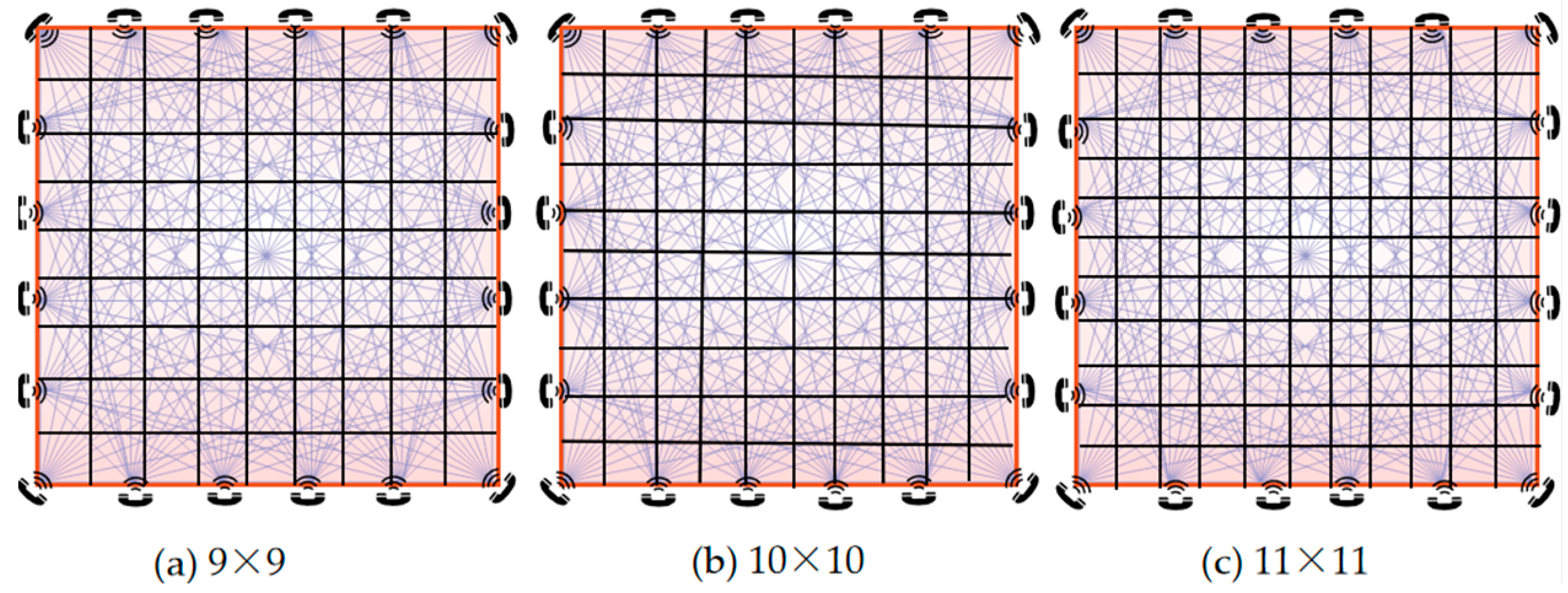
The reconstructed cross section is arranged with 20 acoustic transceiver devices to form 130 effective acoustic paths. The acoustic transceiver arrangement and the formed acoustic paths are shown in Figure 4.
The temperature values in the reconstructed area grids are obtained as solutions to the matrix equation (Equation (3)), and they serve as the basic pixels for ultimate imaging. After preliminary tentative research, combined with previous research in boilers and relevant literature in other fields, three more representative grid division schemes, 9 × 9, 10 × 10, and 11 × 11, were finally determined. The cross-section meshing scheme is illustrated in Figure 5.

3.2.2. Solution Method of the Acoustic Matrix Equation

When the number of rays (the equation number) in the equation does not match the number of grids, Equation (3) becomes a pathological matrix equation, which lacks a definite solution. Various methods have been developed to solve such pathological matrix equations, and iterative algorithms offer advantages such as wide applicability, lower computational complexity, and controllable operation times. Thus, in this study, the LSQR and SART algorithms are employed to solve the reconstructed temperature fields for diverse planes under three meshing schemes. The objective is to investigate the accuracy of the equation solutions using diverse solution methods in each scheme.
(a)
Least Squares QR-Decomposition (LSQR)
Least Squares QR-Decomposition (LSQR) [28,29] is obtained on the basis of Lanczos bidiagonalization (LBD), which can be used to solve the equation ( A T A + λ 2 I ) x = A T b as can the conjugate gradient method. However, when the matrix is sick, the LSQR has a faster convergence rate, higher computational accuracy, and better numerical stability. The optimal solution sequence { x k } is approached by stepwise reduction of the residues r k = b A x k .
(b)
Simultaneous algebraic reconstruction technique (SART)
The SART [30,31] algorithm determines the correction value for a pixel based on the errors of all rays passing through that pixel at the same projection angle, rather than considering only a single ray. The solution process formula for the SART in reconstructing the plane temperature field is as follows:
f j ( k + 1 ) = f j ( k ) + λ 1 i I w i j i I τ i n = 1 N w i n f n ( k ) n = 1 N w i n
where k is iterations, λ is the relaxation factor, f j ( k ) and f j ( k + 1 ) are the j th pixel values in the k th and (k + 1) the sub-iterations, respectively, generally 0 < λ < 2 . The size of the relaxation factor is a factor that affects the reconstruction results and speed. I is the projection index at the projection angle.
Given the non-positive nature of the large matrix equation solved in this paper, the error value of the objective function is set to the termination condition of the SART iteration process. The objective function is the norm of the vector of two solution difference values before and after the iteration. When the error value is less than 1 × 10 7 , the iteration is terminated.

4. Analysis of Reconstruction Results

In order to explore the reliability of the reconstruction effect of fire temperature and fire source location determination under two equation solution methods with three meshing schemes, this paper will study three aspects: cloud map comparison (qualitative), error analysis (quantitative), and fire source location determination results (quantitative).

4.1. Cloud Map Comparison

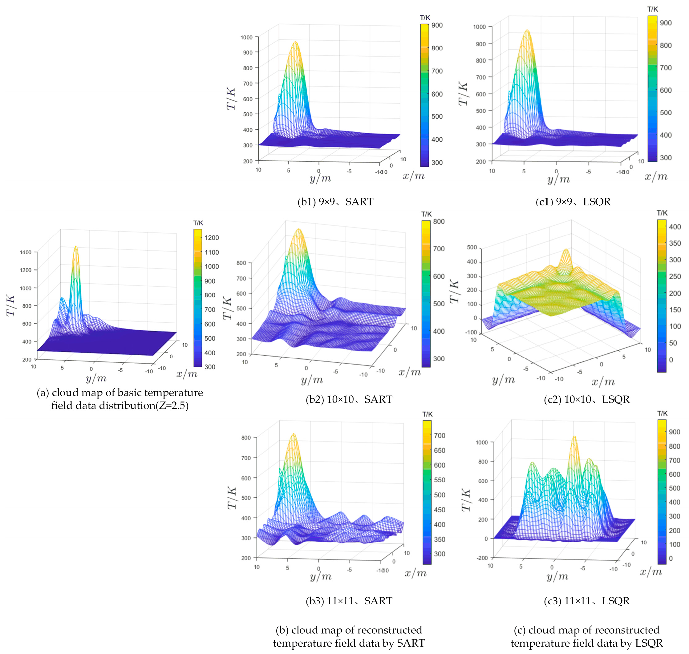
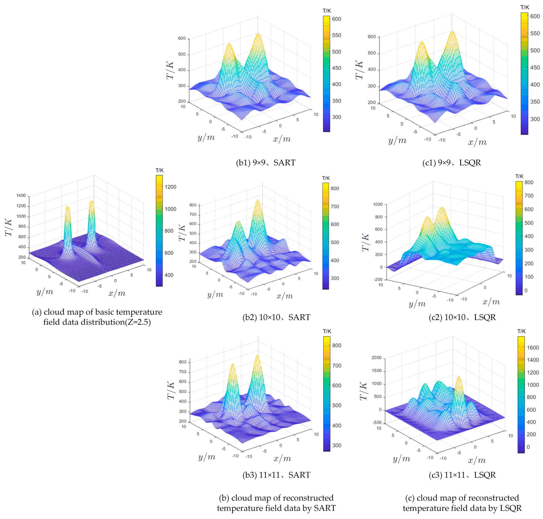
The operating system of the computer performing the iterative process is Windows 10 Professional 64-bit version with a memory capacity of 8192 MB RAM, a processor of Intel(R) Core (TM) i7-8700 CPU @3.2 GHz (12 CPUs), and a main frequency of about 3.2 GHz. Figure 6, Figure 7, Figure 8 and Figure 9 show the results of the temperature reconstruction of a Z = 2.5 section in four fire cases.

4.1.1. Reconstruction Results of Each Scheme under Fire 1 (Close to the Center)

The figure above shows
  • Under the SART, the distributional shape of the reconstructed cloud map under the three different meshing schemes is generally similar to the cloud map of basic temperature field data and shows obvious high temperature areas near the center. However, compared with the basic temperature data, the reconstruction temperature maximum of these three schemes is lower, among which the reconstruction results of the 11 × 11 grid scheme (Figure 6(b3)) are the closest to the basic temperature data.
  • Under the LSQR, the reconstructed cloud map under the three different meshing schemes is significantly different from the basic temperature data cloud map in terms of the distributional shape, temperature maximum value, and coordinates of the high temperature region. Among them, the significant high temperature area appeared in the 9 × 9 grid (Figure 6(c1)) and 11 × 11 grid (Figure 6(c3)) schemes, but the latter has a large deviation from the basic temperature field in the position of the high temperature area. However, the temperature distribution of the 10 × 10 grid (Figure (6c2)) scheme was abnormal, and the reconstruction failed.

4.1.2. Reconstruction Results of Each Scheme under Fire 2 (Close to the Wall)

The figure above shows
  • Under the SART, the distributional shape of the reconstructed cloud map under the three different meshing schemes is generally similar to the basic temperature data, and it shows an obvious high temperature area in the position close to the wall. However, compared with the basic temperature data, the reconstruction maximum temperature of these three schemes is lower, among which the reconstruction results of the 11 × 11 grid scheme (Figure 7(b3)) are the closest to the basic temperature data.
  • Under the LSQR, the reconstructed cloud map under the three different meshing schemes is significantly different from the basic temperature data cloud map in terms of the distributional shape, temperature maximum value, and coordinates of the high temperature region. Among them, the significant high temperature area appeared in the 9 × 9 grid (Figure 7(c1)) and 11 × 11 grid (Figure 7(c3)) schemes, but the latter has a large deviation from the basic temperature field in the position of the high temperature area. However, the temperature distribution of the 10×10 grid (Figure 7(c2)) scheme was abnormal, and the reconstruction failed.

4.1.3. Reconstruction Results of Each Scheme under Fire 3 (Close to the Corner)

The figure above shows:
  • Under the SART algorithm, the distributional shape of the reconstructed cloud map under the three different meshing schemes is generally similar to the basic temperature data and shows obvious high temperature areas close to the corner. However, compared with the basic temperature data, the reconstruction temperature maximum of these three schemes is lower, among which the reconstruction results of the 9 × 9 grid scheme (Figure 8(b1)) are the closest to the basic temperature data.
  • Under the LSQR, the reconstructed cloud maps under three different meshing schemes showed significant differences in the distributional shape, temperature maximum, and coordinates of the high temperature region. Among them, a significant high temperature area appeared under the 9 × 9 grid (Figure 8(c1)) grid (Figure 8(c1)) scheme, while the temperature distribution morphology in the 10 × 10 grid (Figure 8(c2)) and 11 × 11 grid (Figure 8(c3)) schemes was abnormal, and the reconstruction failed.

4.1.4. Reconstruction Results of Each Scheme under Fire 4 (Double Fire Source)

The figure above shows:
  • Under the SART, the distributional shape of the reconstructed cloud map under three different meshing schemes is generally similar to the basic temperature data, and both fire sources show obvious high-temperature areas. However, compared with the basic temperature data, the reconstruction temperature maximum of these three schemes is lower, among which the reconstruction results of the 11 × 11 grid scheme (Figure 9(b3)) are the closest to the basic temperature data.
  • Under the LSQR, the reconstructed cloud maps under three different meshing schemes showed significant differences in the distributional shape, temperature maximum, and maximum coordinates of the high temperature region. Among them, the significant high temperature area appeared in the 9 × 9 grid (Figure 9(c1)) and 10 × 10 grid (Figure 9(c2)) schemes, but the latter has a large deviation from the basic temperature field in the position of the high temperature area. However, the temperature distribution of the 11 × 11 grid (Figure 9(c3)) scheme was abnormal, and the reconstruction failed.
The reconstructed temperature maximum value under the three grid division schemes is relatively low compared with the basic temperature data. On initial consideration, this phenomenon may be caused by the following reasons:
Acoustic CT temperature field reconstruction is a typical inverse problem that requires the interpolation of infinitely many possible solutions with limited measurement data. In this process, the size of the grid division as well as the choice of the interpolation method may have a significant effect on the reconstruction results.
First, the reconstructed temperature data within each grid is determined by the fit of the entire large matrix equation through all ray-averaged velocities within that grid. The high temperature peak point of the basic temperature data usually appears in the local coordinates. If the grid is large at this time, the acoustic rays through the grid may not pass through the coordinate point of the high temperature peak, which is unable to accurately capture the detailed changes of the temperature field, thus leading to low measurement data.
Second, we used cubic spline interpolation in the reconstruction process to reproduce the limited discrete data globally, which may make the data smoother and in turn lead to the loss of high-temperature features of the local coordinate points. This may be another reason for the reconstructed temperature field peak being lower than the base temperature field peak.

4.2. Analysis of Reconstruction Error and Reconstruction Time-Consuming

The accuracy and timeliness of temperature field reconstruction are the key parameters for effectively using the temperature information at the fire site. Next, this paper quantitatively analyzes the reconstruction effect under different reconstruction schemes in four fire situations from these two aspects.

4.2.1. Error Analysis of the Reconstruction

In this paper, the root mean square percentage error [8] is used to evaluate the reconstruction effect. The root mean square percentage error is an indicator to measure the difference between the predicted value and the actual value. It can be calculated by calculating the root mean square error (RMSE) between the reconstructed value and the actual value, dividing by the average value of the actual value and multiplying by 100%. The formula is the following:
R M S P E = 1 N i = 1 N [ T c ( i ) T M ( i ) ] 2 T M ave × 100 %
where N is the total number of grids divided by measured region; T c ( i ) is the reconstruction temperature of the central coordinates of the i th grid; T M ( i ) is the basic temperature of the central coordinates of the ith grid ; and T M ave is the average temperature of the foundation temperature field.
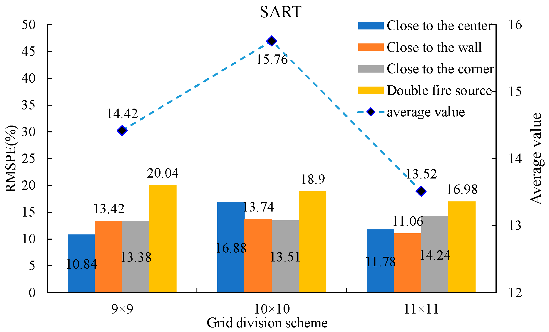
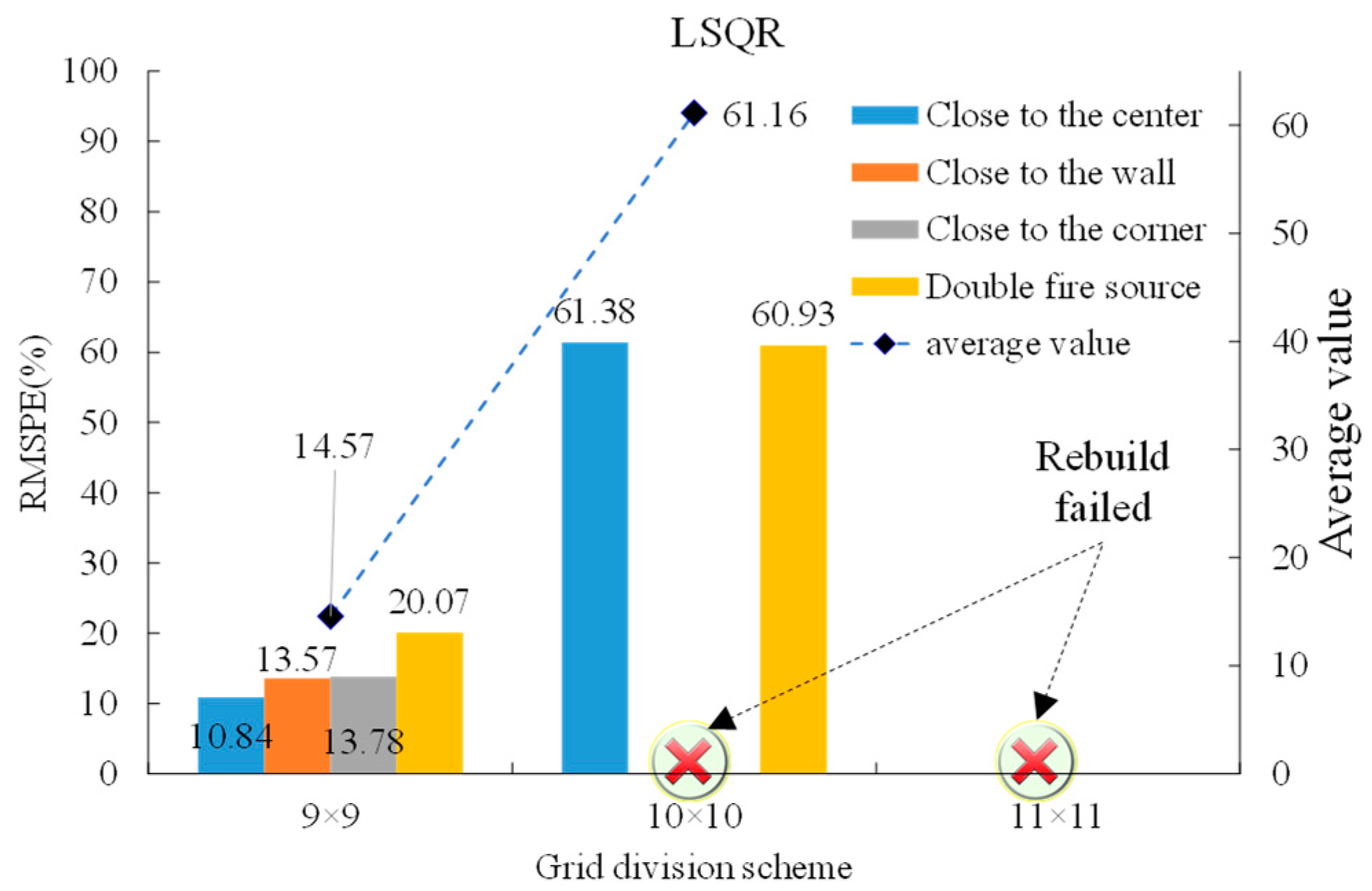
The root mean square percentage error (RMSPE) under each scheme is shown in Figure 10 and Figure 11, Figure 10 and Figure 11 show the reconstruction error data of four fire conditions (close to the center, wall, corner, double fire source) under the grid division schemes, 9 × 9, 10 × 10, and 11 × 11, respectively.
The data show that from Figure 10, under the SART, the reconstruction error RMSPE value of the four fire sites under the three grid division schemes is below 20.04%, and the average error value is 14.42%, 15.76%, and 13.52%, respectively. Under the same grid division scheme, the reconstruction error in the case of a double fire source is higher than that of other single fire sources, which serves to show that the complexity, to some extent, of the distribution pattern of the fire site will affect the reconstruction effect.
According to the data from Figure 11, the reconstruction error of the four fire conditions under 9 × 9 is 14.57%, the reconstruction error of the four fire conditions (close to the center, wall, corner, and double fire source) increases successively, and the overall reconstruction effect is consistent with the 9 × 9 grid division scheme under the SART algorithm. Under the 10 × 10 grid scheme, the reconstruction of the fire conditions by wall and corner failed; the other two reconstruction errors are up to 61.16%; and all reconstruction errors under the 11 × 11 grid division scheme failed.
Therefore, compared with LSQR, SART has higher reconstruction accuracy and better noise resistance; the 11 × 11 grid scheme is better than other reconstruction schemes.

4.2.2. Time-Consuming Analysis of the Reconstruction (Solution of the Equations)

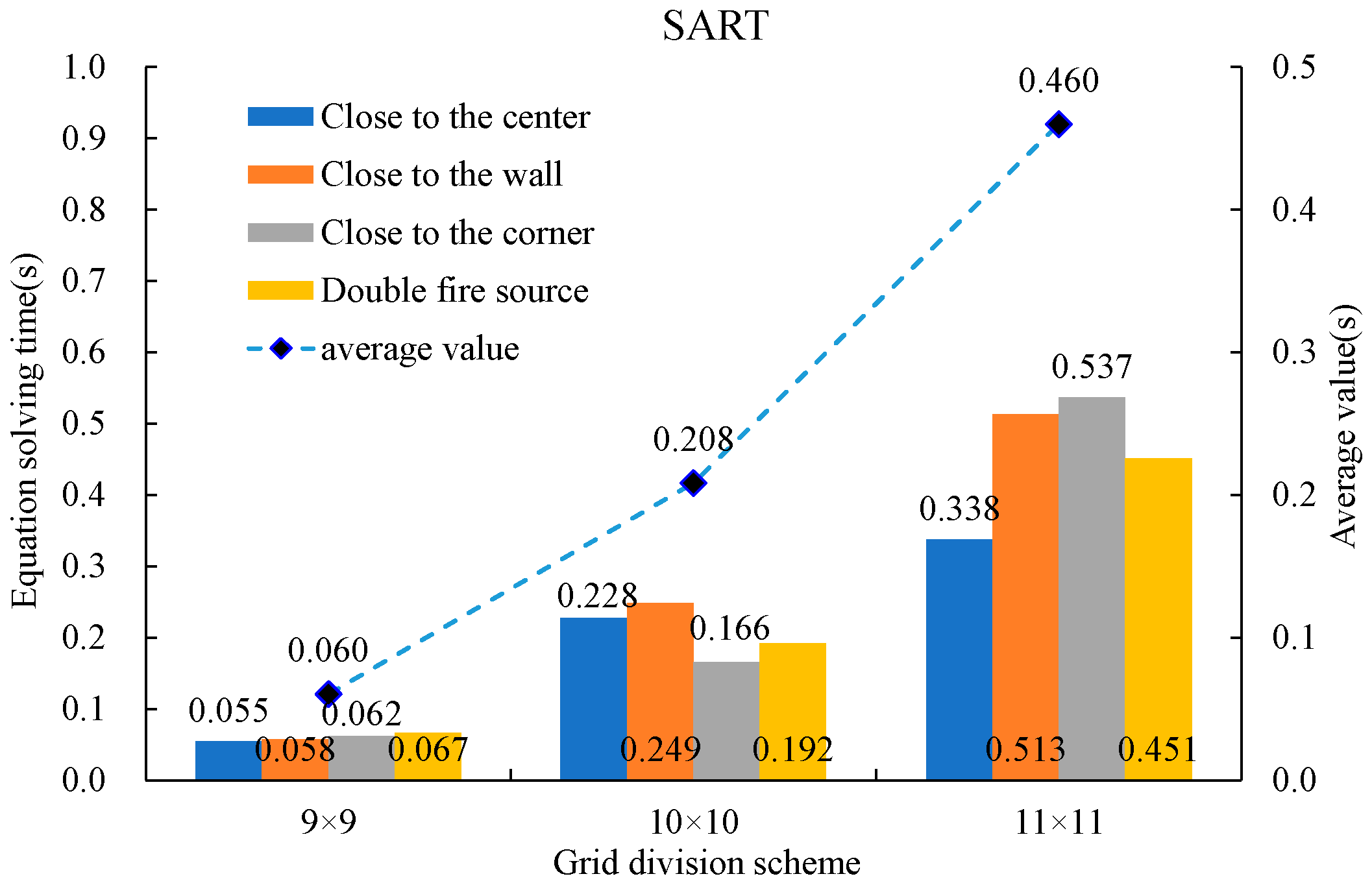
The solution time of the large sparse matrix equation directly determines the timeliness of the fire temperature field reconstruction. Figure 12 and Figure 13 show the time-consuming data of the equation under SART and LSQR, including four fire conditions (close to the center, wall, corner, double fire source) under three grid division schemes (9 × 9, 10 × 10, 11 × 11).
The data presented in Figure 12 shows that: under the SART algorithm, the solution time of the reconstruction equation under different fire locations is different under the same grid scheme, but the difference is not significant, and no regularity is found in this study; but the grid scheme affects the equation solving time more significantly, with the increase of the number of grids being 0.06 s, 0.208 s, and 0.46 s, and the approximate linear relationship increasing.
The data presented in Figure 13 shows that, under the LSQR algorithm, the control of the equation solution time is less than that of the SART algorithm, and the solution time is basically the same. With the increase of grid number, the average solution time (0.017 s, 0.019 s, and 0.022 s) of each scheme also increases, but the increase ratio is small compared with the SART.
Therefore, as from the above analysis:
  • In terms of reconstruction time, the LSQR solution time is in the order of 10−2 s, while the SART solution time is in the order of 10−1 s, so the former has advantages in timeliness.
  • Under the two algorithms, the solution time of the equation under different fire position parameters is slightly different, but the difference is not huge, and there is no obvious regularity.
  • Under the two algorithms, the number of mesh divisions and the solution time have an approximately positive linear relationship. Compared with the LSQR algorithm, the computation time under the SART algorithm is more sensitive to the grid number. The grid increases, and the time consumption increase is more significant.

4.3. Results of Fire Source Location Determination

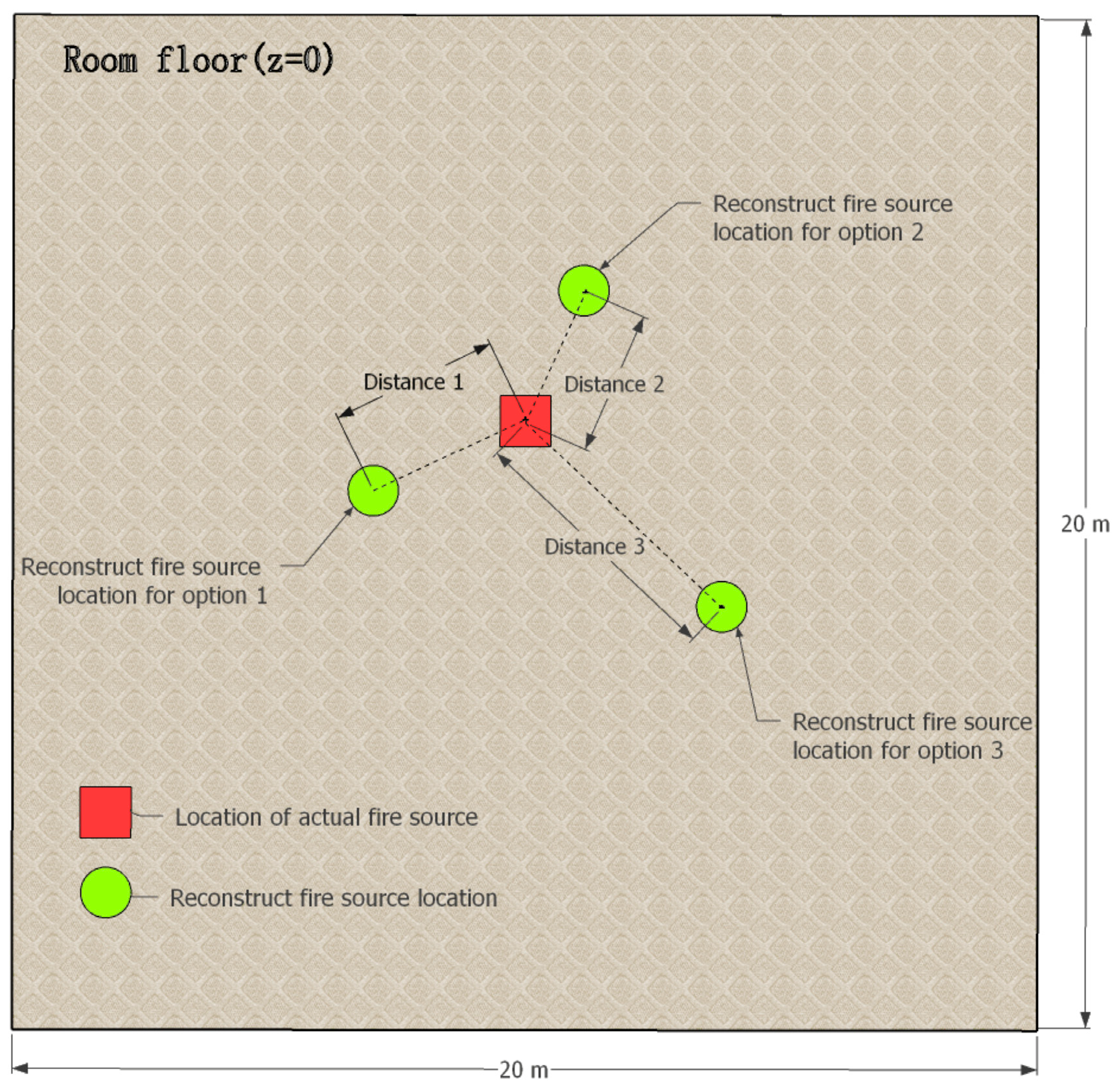
In this article, the reconstructed temperature peak coordinate on the reconstruction section (Z = 2.5) is determined as the fire source position by calculating the distance between “the fire source location determined” and “the fire source location set by numerical simulation”.
The schematic of the location of actual fire source and reconstruct fire source location is shown in Figure 14.
In Figure 14, the red square is the location of the actual fire source, and the yellow round is a reconstruction of the fire source location. “Distance” is the distance between the location of the actual fire source and the reconstruction of the fire source location.
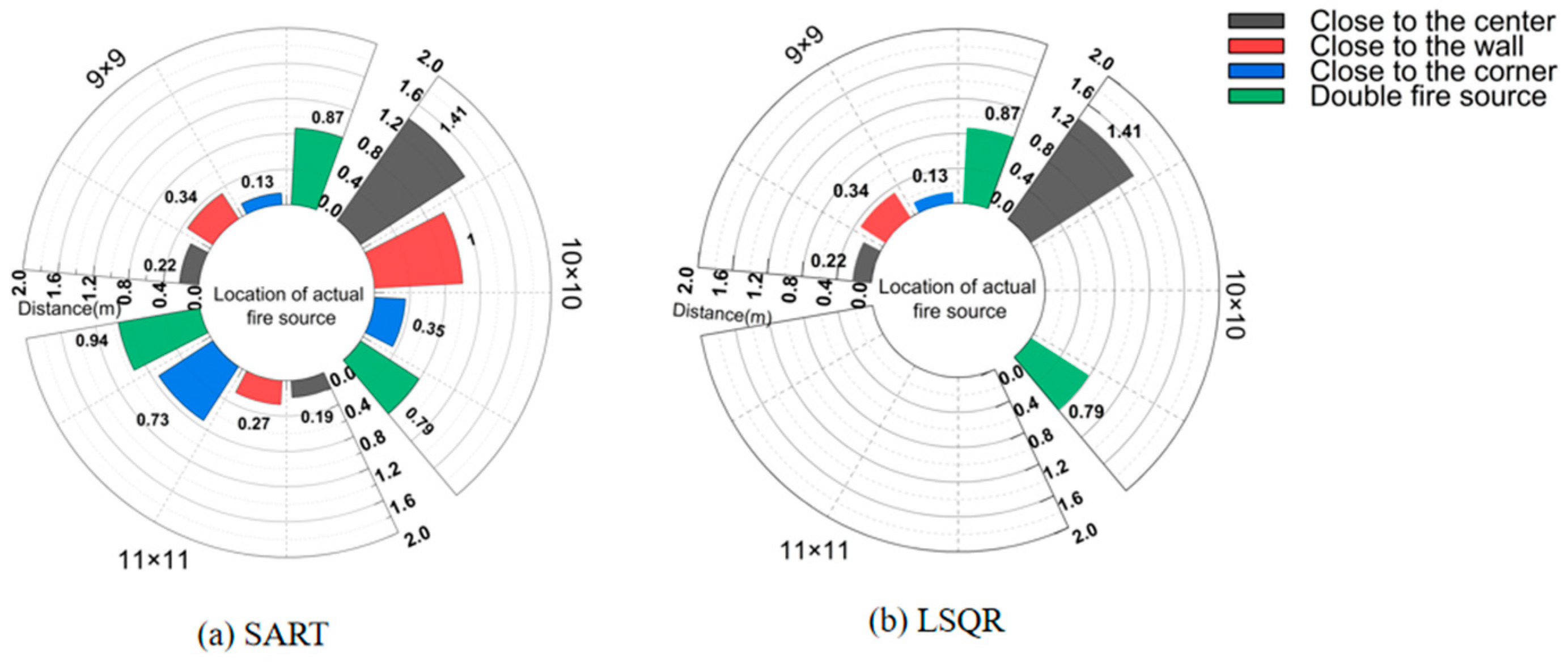
The reconstruction effect of the fire point location of the four fire sites is shown in Figure 15, among which the scheme data in the polar coordinate map is the “Distance” data in the figure above.
In Figure 15, Figure 15a,b show the distance (reconstruction distance) images between the above four fire sites and the base fire sites, respectively, reconstructed by the SART and the LSQR under the three grid division schemes. The failed reconstruction scheme is not shown in the figure. Specifically, the reconstruction distance of two fire sources is the average of the reconstruction distance of two fire sources.
The figure above shows:
Under the 9 × 9 grid scheme, the determination results of SART and LSQR in the four fire sites are basically consistent; the coordinate determination error of a single fire source is within 0.5 m, and the average determination error of double fire sources is 0.87 m. In this scheme, both algorithms can achieve more accurate fire source location determination, and the determination of a single fire source location coordinate is more accurate.
Under the 10 × 10 and 11 × 11 grid schemes, the LSQR cannot determine the fire point location in many cases. However, the SART shows higher robustness, and the judgment error of the position of the fire source is within 1.5 m, which can basically realize the determination of the fire point position.

5. Conclusions

This paper tries to apply acoustic CT temperature measurement technology in the field of building fire to obtain building fire site data information more efficiently and to serve for efficient rescue, emergency evacuation command, and fire accident investigation. Based on the numerical simulation and acoustic CT temperature measurement, the fire point determination effect of building space under various fire point conditions is studied, and the following conclusions are drawn:
  • Under the multi-grid division scheme, the robustness of SART is better than that of LSQR, which can better realize the temperature field reconstruction based on multiple grid schemes at different fire locations.
  • In terms of reconstruction accuracy (root mean square error), SART and LSQR are basically the same under the 9 × 9 grid scheme, but in other schemes, SART is obviously better than LSQR. Under SART, the reconstruction data accuracy of the 11 × 11 grid scheme is the highest.
  • In terms of reconstruction time consumption (equation solving), LSQR is better than SART overall; mesh division number has a significant positive correlation with the time consumption of equation solving.
  • In terms of the determination of fire source location (peak coordinate), SART and LSQR can better realize the determination of fire source location under the 9 × 9 grid scheme. Under the SART, the three grid division schemes can determine the fire source position, but the 9 × 9 grid scheme has the highest judgment accuracy.

Author Contributions

Conceptualization, H.Q. and L.C.; methodology, H.Q.; software, H.Q.; validation, H.Q., L.C., X.Y., Z.G. and H.Y.; formal analysis, H.Q.; investigation, H.Q.; resources, H.Q.; data curation, L.C.; writing—original draft preparation, H.Q. and L.C.; writing—review and editing, H.Q. and L.C.; supervision, H.Q., L.C., X.Y., Z.G., H.Y., Z.L., H.S., Z.B. and J.W.; project administration, H.Q.; funding acquisition, H.Q. All authors have read and agreed to the published version of the manuscript.

Funding

This work was supported by Henan Province Key R&D Special Project (231111322200), Henan Province Science and Technology Tackling Key Problems Projects (232102320232) and the Natural Science Foundation of Henan (232300420317).

Institutional Review Board Statement

Not applicable.

Informed Consent Statement

Not applicable.

Data Availability Statement

The authors declare that the data supporting the findings of this study are available within the article.

Conflicts of Interest

The authors declare no conflict of interest.

References

  1. Zhang, J.W.; Cui, Y.H.; Zhou, J.G. Analysis and identification of ignition points and ignition sources. Fire Sci. Technol. 2011, 30, 973–976. [Google Scholar]
  2. Deng, Y.C. Investigation and analysis of a warehouse fire accident. Fire Sci. Technol. 2006, 6, 832–834. [Google Scholar]
  3. Florin, M.; Emilian, G.; Cornel, M.S.; Maria, P.; Loan, N.V.; Sonia, N.S.; Titus, V. FDS results for selecting the right scenario in the case of a building fire: A case study. Fire 2022, 5, 198. [Google Scholar]
  4. Khan, A.E.; Ahmed, A.M.; Khan, H.E.; Majumder, C.S. Fire Emergency Evacuation Simulation of a shopping mall using Fire Dynamic Simulator (FDS). J. Chem. Eng. 2017, 30, 32–36. [Google Scholar] [CrossRef]
  5. Suhaimi, S.N.; Ibrahim, A.; Mustapha, S.; Adam, M.N.; Baharuddin, R.M. Development of a smoke prediction model using numerical simulations. Int. J. Comput. Aided Eng. Technol. 2021, 14, 477–492. [Google Scholar] [CrossRef]
  6. Li, S.F. Application and practice of drones in firefighting and rescue work. China Equip. Eng. 2023, 8, 8–10. [Google Scholar]
  7. Chen, B. Research on the application of firefighting drones in high-rise building fire rescue. Fire Community (Electron.) 2022, 8, 45–47. [Google Scholar]
  8. Li, Y.Q.; Liu, S.; Inaki, H.S. Dynamic Reconstruction Algorithm of Three-Dimensional Temperature Field Measurement by Acoustic Tomography. Sensors 2017, 17, 2084. [Google Scholar] [CrossRef]
  9. Zhang, S.P.; Shen, G.Q.; An, L.S.; Niu, Y.G. Online monitoring of the two-dimensional temperature field in a boiler furnace based on acoustic computed tomography. Appl. Therm. Eng. 2015, 75, 958–966. [Google Scholar] [CrossRef]
  10. Yan, H.; Ma, Z.; Zhou, G.Y. Acoustic tomography system for online monitoring of temperature fields. IET Sci. Meas. Technol. 2017, 11, 623–630. [Google Scholar] [CrossRef]
  11. Chen, Y.T.; Yan, H. Reconstruction of complex temperature field based on improved Tikhonov regularization. J. Phys. Conf. Ser. 2021, 1754, 012207. [Google Scholar] [CrossRef]
  12. Yan, H.; Zhuang, Q.; Wang, X.N. Simulation of acoustic CT reconstruction for temperature distribution of stored grain. J. Shenyang Univ. Technol. 2015, 37, 662–666. [Google Scholar]
  13. Yan, H.; Dou, H.; Chen, G.N.; Yao, L. 3D temperature field reconstruction based on the interpolation of 2D acoustic reconstructions. In Fifth International Conference on Machine Vision (ICMV 2012): Algorithms, Pattern Recognition, and Basic Technologies, Proceedings of the Fifth International Conference on Machine Vision (ICMV 2012), Wuhan, China, 20–21 October 2012; SPIE: Bellingham, WA, USA, 2013; Volume 8784, pp. 878422-1–878422-6. [Google Scholar]
  14. Zhong, Q.H.; Chen, Y.S.; Zhu, B.; Liao, S.H.; Shi, K.B. A temperature field reconstruction method based on acoustic thermometry. Measurement 2022, 200, 111642. [Google Scholar] [CrossRef]
  15. Yan, H.; Li, K.; Wang, S.H. A 3D Temperature Field Reconstruction Algorithm Based on Acoustic Travel-Time Tomography. Lect. Notes Electr. Eng. 2012, 140, 639–644. [Google Scholar]
  16. Song, Z.Q.; Fan, X. Detection technology and application of temperature field in boiler based on acoustic method. Boil. Technol. 2005, 1, 20–23+69. [Google Scholar]
  17. An, L.S.; Wang, R.; Shen, G.Q.; Zhang, S.P. Simulation study of acoustic CT algorithm for reconstructing 3D temperature field in furnace. J. Chin. Soc. Power Eng. 2015, 35, 13–18. [Google Scholar]
  18. Yan, H.; Chen, G.N.; Yang, Q.; Liu, L.J. Research on acoustic CT reconstruction of complex temperature fields. Acoust. J. 2012, 37, 370–377. [Google Scholar]
  19. Wang, S.H.; Yan, H.; Li, S. Design of layout for acoustic tomography imaging sensor. China Sci. Technol. Pap. 2014, 9, 413–416. [Google Scholar]
  20. Qin, H.J.; Wen, J.Q.; Gao, Z.H.; Chai, L.L.; Yao, H.W. Preliminary Study on Reconstruction of Building Thermal Field Based on Iterative Algorithm Acoustic CT. Fire 2023, 6, 199. [Google Scholar] [CrossRef]
  21. Wang, R. Acoustic Measurement of Three-Dimensional Temperature Field in Furnace and Its Application in Combustion Optimization; North China Electric Power University: Beijing, China, 2015. [Google Scholar]
  22. Ru, Y.D. Algorithm Research on Acoustic Reconstruction of Three-Dimensional Temperature Field in Furnace. Master’s Thesis, North China Electric Power University, Beijing, China, 2015. [Google Scholar]
  23. Huang, Z.A.; Meng, Y.R.; Yang, R.; Wang, S.Y. Numerical simulation of a cinema fire based on FDS. Int. J. Simul. Process Model. 2018, 13, 200–209. [Google Scholar] [CrossRef]
  24. Zhao, G.; Beji, T.; Merci, B. Study of FDS simulations of buoyant fire-induced smoke movement in a high-rise building stairwell. Fire Saf. J. 2017, 91, 276–283. [Google Scholar] [CrossRef]
  25. Zhao, X.L.; Wei, S.Y.; Chu, Y.Y.; Wang, N. Numerical Simulation of Fire Suppression in Stilted Wooden Buildings with Fine Water Mist Based on FDS. Buildings 2023, 13, 207. [Google Scholar] [CrossRef]
  26. Lu, S.L.; Li, Q.P.; Bai, L.; Wang, R. Performance predictions of ground source heat pump system based on random forest and back propagation neural network models. Energy Convers. Manag. 2019, 197, 111864. [Google Scholar] [CrossRef]
  27. Zhang, D.W.; Li, W.L.; Wu, X.H.; Lv, X.F. Application of simulated annealing genetic algorithm-optimized back propagation (BP) neural network in fault diagnosis. Int. J. Model. Simul. Sci. Comput. 2019, 10, 1950024. [Google Scholar] [CrossRef]
  28. Chen, S.X.; Xiong, H.L.; Liao, J.; Zhou, J.W.; Zuo, J.S. A joint optimization matching tracking algorithm based on CGLS and LSQR. J. Autom. 2018, 44, 1293–1303. [Google Scholar]
  29. Han, H.; Wu, L.N. Decision feedback equalizer based on LSQR algorithm and windowing technique. J. Circuits Syst. 2010, 15, 117–121. [Google Scholar]
  30. Zhang, S.; Zhou, P.; Pan, K.; Liu, Z.G.; Li, Y.D. A SART algorithm for area integral model in desktop micro-CT system. Nucl. Inst. Methods Phys. Res. A 2019, 955, 163288. [Google Scholar] [CrossRef]
  31. Zhu, X.Y.; Zhang, B.; Li, J.; Xu, C.L. 3D flow field reconstruction of a single optical field camera based on pre-recognition technology and SART algorithm. J. Eng. Thermophys. 2020, 41, 1445–1451. [Google Scholar]
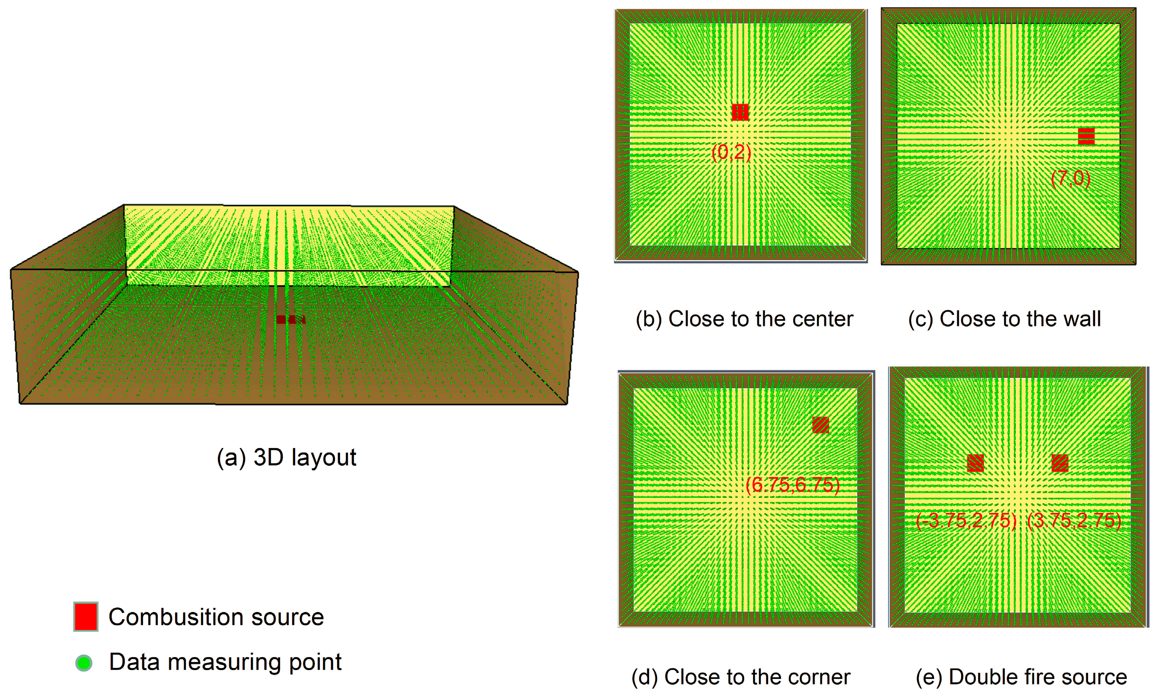
Figure 1. Fire source location.
Fire 06 00353 g001
Figure 2. Basic temperature field fitting model based on the BP neural network.
Fire 06 00353 g002
Figure 3. Temperature field distribution and fitting effect of X = 0 and Z = 5 section foundation of fire.
Fire 06 00353 g003
Figure 4. Acoustic wave transceiver layout of the cross-section and the formed acoustic wave path.
Fire 06 00353 g004
Figure 5. Grid division schemes.
Fire 06 00353 g005
Figure 6. Reconstruction of the cross-section of fire 1.
Fire 06 00353 g006
Figure 7. Reconstruction of the cross-section of fire 2.
Fire 06 00353 g007
Figure 8. Reconstruction of the cross-section of fire 3.
Fire 06 00353 g008
Figure 9. Reconstruction of the cross-section of fire 4.
Fire 06 00353 g009
Figure 10. Root Mean Square Percentage Error (RMSPE) under each reconstruction scheme (SART).
Fire 06 00353 g010
Figure 11. Root Mean Square Percentage Error (RMSPE) under each reconstruction scheme (LSQR).
Fire 06 00353 g011
Figure 12. Time-consuming data for equation solving under each reconstruction scheme (SART).
Fire 06 00353 g012
Figure 13. Time-consuming data for equation solving under each reconstruction scheme (LSQR).
Fire 06 00353 g013
Figure 14. Schematic diagram of the real fire source location and the reconstructed fire source location.
Fire 06 00353 g014
Figure 15. The distance between the reconstructed fire point location and the basic fire point location.
Fire 06 00353 g015
Table 1. Key parameter settings for numerical simulation.
FireLocation of Fire Source (m)Overall Size (m³)Mesh Size (m³)Fire Source Size (m2)Initial Temperature (K)Burning
Material
Ignition Source Power (kW/m2)
Close to the center(0,2,0)20 × 20 × 50.5 × 0.5 × 0.51.5 × 1.5293.15Polyurethane
_GM27
8000
Close to the wall(7,0,0)
Close to the corner(6.75,6.75,0)
Double fire source(−3.75,2.75,0),
(3.75,2.75,0)
Table 2. The specific value of the correlation coefficient and the relative error distribution.
FireCoefficient of
Determination R
Center Value of Error (K)Error Distribution Proportion
Close to the center0.994722.06893%
Close to the wall0.995076.18993%
Close to the corner0.99726−0.95193%
Double fire source0.99607−7.86880%
Table 3. Reconstruction key parameter settings of the tested cross section.
Reconstruction PlaneSize of the Plane (m2)Grid DivisionNumber of Acoustic
Transceivers
Number of Valid Paths
Z = 2.520 × 209 × 9, 10 × 10, 11 × 1120130
Disclaimer/Publisher’s Note: The statements, opinions and data contained in all publications are solely those of the individual author(s) and contributor(s) and not of MDPI and/or the editor(s). MDPI and/or the editor(s) disclaim responsibility for any injury to people or property resulting from any ideas, methods, instructions or products referred to in the content.