Article

Downwind Fire and Smoke Detection during a Controlled Burn—Analyzing the Feasibility and Robustness of Several Downwind Wildfire Sensing Modalities through Real World Applications

1
Gridware Technologies Inc., Walnut Creek, CA 94597, USA
2
Electrical Engineering and Computer Sciences Department, University of California, Berkeley, CA 94720, USA
3
Disaster Lab, College of Engineering, University of California, Berkeley, CA 94720, USA
*
Author to whom correspondence should be addressed.
Fire 2023, 6(9), 356; https://doi.org/10.3390/fire6090356
Submission received: 21 August 2023 / Revised: 8 September 2023 / Accepted: 9 September 2023 / Published: 12 September 2023
(This article belongs to the Topic Application of Remote Sensing in Forest Fire)

Abstract

:
Wildfires have played an increasing role in wreaking havoc on communities, livelihoods, and ecosystems globally, often starting in remote regions and rapidly spreading into inhabited areas where they become difficult to suppress due to their size and unpredictability. In sparsely populated remote regions where freshly ignited fires can propagate unimpeded, the need for distributed fire detection capabilities has become increasingly urgent. In this work, we evaluate the potential of a multitude of different sensing modalities for integration into a distributed downwind fire detection system, something which does not exist today. We deployed custom sensor-rich data logging units over a multi-day-controlled burn event hosted by the Marin County Fire Department in Marin County, CA. Under the experimental conditions, nearly all sensing modalities exhibited signature behaviors of a nearby active fire, but with varying degrees of sensitivity. We present promising preliminary findings from these field tests but also note that future work is needed to assess more prosaic concerns. Larger scale trials will be needed to determine the practicality of specific sensing modalities in outdoor settings, and additional environmental data and testing will be needed to determine the sensor system lifetime, data delivery performance, and other technical considerations. Crucially, this work provides the preliminary justification underscoring that future work is potentially valuable and worth pursuit.

1. Introduction

Evidence from historical wildfire trends predicts increasing fire severity with “six of California’s seven largest wildfires [erupting] in the past year” [1]. The causes and conditions that have led to the increased fire activity are numerous (e.g., drought conditions, electric grid equipment failure, etc.), but the consequences are clear: staggering economic losses, property and ecological damage, and loss of life. One example is the California Camp Fire of 2018, which resulted in over USD 16 billion in damages over two weeks and a loss of 86 lives [2]. A large number of these fires occur in what is known as the wildland–urban interface (WUI), the zone of transition between wildland and human development [3]. Fires that start in this WUI zone have the potential to go undetected for a longer period of time than ignitions in urban areas due to a reduced population density in these zones, reduced coverage of security cameras, and the potential for ignitions to start out of line-of-sight from residences or businesses. This potential delay in ignition detection can give wildfires an opportunity to grow in size and unpredictability, which reduces the ease of containment. Under such circumstances, the importance and need for remote fire detection capabilities in these zones have become paramount.
Low-cost, low-power distributed sensor networks have become a promising avenue in achieving early wildfire detection capability [4,5,6,7,8,9]. If implemented in practice, such a system would supply fire fighting forces with an early warning of freshly ignited fires, knowledge of localized geography-specific environmental details, and real-time situational awareness of how the fire is expanding or moving. However, these systems need to be tested to prove their detection capabilities across a variety of parameters, and for that, we need to test them in live fire situations, which is most feasible under the quasi-controlled setting of a controlled burn. In this paper, we investigated a wide variety of sensors including optical, infrared, chemical, and sound sensors in order to compare the efficiency and robustness across sensor modalities in a controlled burn situation. We placed the sensors downwind from the fire to ensure that the sensors that rely on particulate or gas detections could collect data. In an actual deployment, there would be the deployment of a sensor node with sufficient and in an appropriate layout to address the highly variable wind intensities and directions during a fire. Evaluating a full node is planned for future research.
Controlled burns are a burning method used to control vegetation in a given area for esthetic, restorative, precautionary, and/or training purposes. These burns can be used to create diverse habitats for plants and animals, reduce fuels, thereby preventing more destructive fires, and as training exercises for departments to better understand the nature of wildfires and how to effectively deal with them. This study deployed sensors at the Marin County Fire Department’s controlled burn in Novato, CA in May 2021 for fuel reduction purposes [10]. While controlled burns are of a lower intensity than uncontrolled wildfires, adapting sensor systems to data collected from these events will ensure that the sensors are sensitive enough to detect early fire starts in wildfire situations.
In this paper, we review the academic research and commercial applications focused on sensing modalities for fire detection. We also present the custom sensing unit that we built based on these findings and provide an overview of our experimental setup during the controlled burn. Then, we discuss our results including areas where we have room for improvement in collecting more diverse and wildfire-representative data during future controlled burns.

1.1. Related Work

Research into sensors for fire detection can be broadly grouped into remote sensing and local sensing. The remote sensing of wildfires today is primarily electromagnetic sensor-based [11]. The main limitation with remote sensing is that occlusions such as terrain line-of-sight limitations or volatile weather patterns (e.g., fog and rain) can impede the capabilities of the system. In contrast, for local sensing (often also referred to as ground-based or in situ sensing), the sensors need to be near a fire and/or its emissions to detect it reliably. Local sensing can include detectors for gas, particulate matter, localized humidity, sound, radio frequency, and wind, among others. Given the dependency on proximity, topography, and wind dynamics, the local sensing of wildfires often requires a large number of units to cover any appreciable land area, and these are thus often called sensor nodes or networks and involve a wireless mesh network.
This review focused on sensor nodes because they are the least expensive to implement and design compared to other methods for wildfire detection [12]. Sensor nodes are placed throughout a wildfire risk area to form a wireless sensor network (WSN). The sensors transmit data through the network to a base station where they are processed to detect fires. Once detected, notice may be sent out to the authorities for verification and response.
Below, we briefly review the specific sensor technologies we included in our sensor package evaluation.

1.2. Optical Sensors (Cameras)

Many fire-detection systems employ camera-based techniques because they are the most intuitive sensing modality for operators to understand and can monitor a large area of land with just one unit. Camera systems can use pan-tilt-zoom (PTZ) cameras or multiple static cameras where the images are stitched together so that a single unit can have 360-degree visibility. Because these systems can easily employ high-resolution cameras, they often use machine learning techniques to identify specific characteristics of a wildfire (e.g., contrast, flicker, temporal patterns, etc.) and give operators automated alarms coupled with snapshots for further validation [13]. However, this means that the system needs to have line-of-sight to the target area, which may not be possible in every installation, and this type of system either needs to be coupled with local detection units or several units need to be distributed to limit blind spots. An additional concern with these types of systems is the power requirements of capturing, processing, and potentially delivering a real-time video feed to remote observers or edge computation nodes. The power requirements of such systems can be prohibitive for certain remote installations that do not have access to the electrical grid and prohibit large energy harvesting installations (e.g., photovoltaics). Finally, an obvious concern with camera techniques is privacy since, ideally, the system would have visibility of a large area of land, which also means that it can collect visual information on non-wildfire-related human activity that has the potential of being exploited.
One approach to identify whether there is a wildfire in the scene is to look at individual or clusters of pixels to identify flame flicker, which exists in the visible and infrared spectra [13]. This approach takes into consideration the unique temporal characteristics of fire, which is more accurate than just classifying a single image but is less reliable at long distances [14]. Similarly, the same can be classified from a single photodiode if exposed to a fire, particularly if equipped on a distributed fire detection system looking to classify wildfire flicker from tens of meters away. Using a cheap COTS NIR flame flicker at nighttime, a candlelight flicker could be detected from 10 m away, while the daytime performance was significantly worse [15]. Commercial non-camera-based flame detectors look for flicker between 1 and 10 Hz. These commercial systems also tend to incorporate an ultraviolet (UV) sensing component to mitigate any noise that may occur from intermittent sunlight exposure.
In the commercial space, the Lindsey FireSense FIREBird system is a camera-based system that uses an array of cameras for a 360-degree field-of-view (FOV) [16]. The system also uses additional thermal and environmental sensors to aid in fire detection. The company claims it can detect a 3 ft × 3 ft fire from 400 feet or a large fire from a half-mile away. The IQ FireWatch system is similar, but its imager covers a larger spectral range that offers improved performance for nighttime use [17]. They claim that their system can detect smoke plumes up to 40 miles away in perfect weather conditions, but the performance can be significantly impeded by fog or clouds. The Lesnoy Dozor is a similar system based in Russia, while the FireHawk system is one geared for timber plantations that uses a rotating camera for a full panoramic image [18,19]. These two systems suffer the same drawbacks as the others above-mentioned in that they require installation at significant heights, clearing the tree-line, and achieving line-of-sight visibility to ignition sites.

1.3. Temperature

Temperature fluctuations from a wildfire result from conduction, convection, and radiation, but for early detection sensing purposes, convection and radiative heating are the most relevant [20]. Radiative heating and convective heating during a wildfire demonstrate very different response curves, with radiative heating increasing monotonically as a fire approaches, and convective heating demonstrating significant increases in variance, but not necessarily in mean temperature, as cooling air can be drawn toward fire [21]. Researchers from Bilkent University confirmed this when they performed several fire experiments where they placed several COTS sensor units at varying distances from a fire source and measured the temperature [22]. They noticed that the sensor units that were placed downwind saw greater temperature spikes due to convective heat transfer from the combustion. For an early detection system, however, the fire ideally has not yet reached the level at which it is causing significant convective heat fluctuations due to fire-generated wind currents.
For a smoldering fire, the peak electromagnetic emission is within the infrared domain, 1–5 µm [13]. Cheap, single-pixel infrared detectors exist (i.e., thermopiles) that can be tailored to specific wavelengths with additional optical filters that can correspond to ranges indicative of a wildfire. One problem with this approach is that the exhaust of a wildfire is composed of a variety of matter that can attenuate any incident infrared radiation from the fire [23]. However, if the attenuation bands of the constituent parts of wildfire exhaust are known, a multiband system that can look at several wavelengths can be created to estimate the wildfire temperature or look specifically for the constituent attenuation bands to obtained an estimate of the amount of smoke being exhausted within the sensor’s FOV. By knowing that one of the attenuation bands for CO2 is around 4.3 µm [24], a system can be created to look at a reference band (e.g., 4.0 µm) and the CO2 attenuation band to create an alarm for the presence of a large concentration of CO2.

1.4. Humidity

Relative humidity can increase during wildfires due to the release of water vapor during combustion. Water vapor is released from wildfires through two processes: the chemical output of hydrocarbon combustion, and the evaporation of water from woody biomass due to conductive heat [21,25,26]. Both mechanisms together cause detectable spikes in humidity during the initial phases of combustion. Byram [27] developed a simplified oxidation reaction for generalized biomass (C6H9O4) as follows:
4C6H9O4 + 25O2 + [0.322MH2O + 94N2]→18H20 + 24CO2 + [0.322MH2O + 94N2] + 11.6 × 10⁹ J
Moisture percentage of the fuel is represented by M (included in the brackets with atmospheric nitrogen as inert components of the reaction). As a simplified formula, it does not include the range of additional combustion emissions from wildfires beyond the basic oxidation reaction assuming complete combustion (note no CO in oxidation products due to this assumption). With this formula, Byram posits that for fuel moisture levels below 57%, the majority of water vapor from a wildfire is due to the combustion chemistry of the biomass hydrocarbons.
Humidity sensors have been widely employed in multi-sensor wildfire detection systems, but most studies have not specified the relative importance of humidity sensors in overall system accuracy [28,29]. Nonetheless, capacitive humidity sensors are quite common in multi-sensor wildfire detection systems being developed in academia and the commercial sector, most likely because of the clear role of moisture in biomass combustion, as noted above.

1.5. Wind

Wind sensors (anemometers) are commonly used by firefighters responding to large wildfires due to the risks associated with sudden changes in wind direction for active firefighting [30]. These anemometers are most often used to predict fire front movement on live wildfire incidents, and not to detect new spot fires or engage in the early detection of a new wildfire. Wind sensors have likewise been less often used in academic research aimed at the early detection of wildfires [29,31]. They are commonly used in fire prediction and forecasting models due to the key role wind speed plays in fire risk [32,33]. Heat fluctuations from wildfires can influence wind currents in close proximity to the fire, but it is unclear at what stage of fire these winds are first evident. If they are evident at feasibly detectable levels at the earliest stages of fire, this could potentially be relevant for early detection in very remote areas or during times of significant atmospheric occlusion of other sensors.
Basic wind sensors typically detect wind via anemometers. Another way that the wind intensity, direction, and changes can be detected is via a spatially distributed system detecting the evolving levels of relative humidity, temperature, PM, and gases over time. Local wind dynamics can potentially be inferred from the spatially distributed temperature, humidity, smoke, or other sensors detecting localized variations driven by fire with sufficient time intervals over a short period of time to detect granular changes [34]. The downside is that it is hard to differentiate the temperature and humidity fluctuations driven by close proximity to fire (radiant heat and water vapor release) from those driven by wind (wind-carried heat convection and increased humidity). This approach would therefore most likely be applicable beyond a minimum distance from the fire.

1.6. Particulate Matter

During combustion, an extensive variety of particulate matter (PM) is released, alongside gases [35,36]. The relative proportions of these quantities vary depending on the fuel source and environmental characteristics [13]. Burning biomass generates a higher proportion of PM 2.5 compared with coarser particulate matter [37]. One mass emission estimate ratio (grams of emission/kilogram of fuel burned) puts PM 2.5 at 10.3, while particulates between 2.5 µm and 10 µm are at 1.9 and anything larger is estimated at 3.8 [38]. These numbers vary depending on the type of fuel being burned (e.g., biomass, hydrocarbons, etc.) [8]. Some fine particulate components such as levoglucosan (1,6-anhydro-‚-D-glucopyranose) have been demonstrated to be a decent biomarker for biomass combustion emissions, and thus holds potential for sensors appropriately tuned to its detection [39]. A distributed fire detection system that uses a particulate counter as one of its modalities also serves the dual purpose of characterizing the air quality across a geographical region, which is an important feature for complex microclimate environments such as the San Francisco Bay Area, where the air quality can vary greatly across the metropolitan area. These systems have become low cost, are increasingly widespread through many WUI areas, and have been shown to be strongly correlative with PM reference instruments when correction equations for each package are implemented [40]. PurpleAir is one company offering low-cost particulate counters for consumers and is making that data publicly accessible for anyone to view [5]. This is a valuable offering for people wanting to monitor their local air quality and for informing computational models of wildfire particulate diffusion.

1.7. Gas

The top three exhaust constituents from wildfire by mass are CO2 (71.44%), water (20.97%), and CO (5.52%) [38]. NOx is also generated in significant quantities. Therefore, having CO2, CO, and NOx sensors could potentially increase the detection capabilities of any fire detection system. In a wildland fire setting, one general limitation will be the diffusion rate of these gases across an area and, in the case of sensors that require direct contact with the gas, the location of the sensor in relation to the fire and wind direction. Additionally, for CO2, the additive concentration of CO2 from the ignition source must be substantial enough to be detectable against high normal concentrations of CO2 in the atmosphere and confounding sources of CO2. NOx and CO do not suffer from this last drawback, as background concentrations in the atmosphere are very low, particularly in remote wildland contexts where early detection would be the most difficult. The most common sensors employed for CO detection are non-dispersive IR absorption (NDIR), electrochemical, and metal-oxide-based sensors. Although MOS sensors are widely used for gas sensing and have been used in other fire detection system prototypes, they are less ideal for use in distributed low-power systems because of the power requirements of the built-in heater module [41]. Alternative non-dispersive infrared (NDIR) sensing techniques exist where the attenuation at specific electromagnetic wavelengths is measured, which can be correlated to the attenuation of a specific gas, therefore indicating the concentration of a particular gas [42]. This method is far superior due to its simpler architecture (i.e., an emitter and receiver diode pair) and lower power requirements. GCxGC is also used to identify the compounds within wildfire smoke. Seventy-two gas phase and 240 particle phase compounds were analyzed using GcxGC to explore the profile of wildfire smoke [43]. Diterpenoids were found to be the most abundant organic particles detected in the wildfire smoke samples. Furthermore, monoterpenes in the gas phase were higher in the wildlife smoke samples compared to the lab smoke samples, which means that they can be used to identify wildfire.
Organic aerosols (OAs) and brown carbon (BrC) are also present in wildfire smoke and can be used to quantify primary and secondary biomass burning. Phenolic compounds and their oxidation products are also large contributors to brown carbon (BrC) ABs405 in wildfire plumes [44], which can be identified with an aerosol mass spectrometer. OAs can be quantified using a photoacoustic absorption spectrometer. Fourier transform infrared spectroscopy (FTIR) can also be used to identify trace gas emissions from burning biofuels [45]. FTIR is especially strong in measuring both organic and inorganic compounds and providing information on the distribution of emitted carbon. Some understudied emissions from wildfires such as polycyclic aromatic hydrocarbons, intermediate-volatile compounds, and alkyl amines require more research given their toxicity and the increasing exposure of populations to biomass smoke [46]. Knowing the emission profile of wildfire smoke is important and can aid in the future modeling of wildfires or exposure assessments.

1.8. Sound

Wildfires have a specific sound associated with them that can indicate not only the presence of a fire but also the type of fire it is. Khamukhin and Bertoldo [47] attempted to create a system that can classify two types of forest fires: crown and surface. Crown fires occur when surface fires spread and ignite the forest canopy, leading to strong turbulent air vortices that result in an increased rate of combustion. Surface fires tend to have a low rate of spread (0.5 m/min) while crown fires tend to be very volatile, extremely dangerous, and can have rates of spread in excess of 200 m/min. Khamukhin and Bertoldo [48] analyzed several open-source wildfire recordings and noticed that the frequency response of a surface fire resembled that of the red noise spectrum while that of a crown fire was more distinct, with a Gaussian distribution centered around 350 Hz. Therefore, for a microphone array placed in the wild, it is possible to classify and triangulate certain fire types to estimate severe wildfire regions. Thompson et al. [49] performed an acoustic analysis of firebrands on a crown fire in Alberta, Canada. This research is especially pertinent because prior studies on firebrands focus solely on structure fires. The audio files from eleven cameras recording the fire were extracted and analyzed, and they found that the in-fire cameras had a low false negative rate of 15% and an even lower false positive rate of 1%. They developed a spatial estimate for the spread of firebrands and concluded that there was the highest amount of firebrands 75 m away from the source, with a concentration of 640 firebrands per kg of tree fuel consumed. This research encourages the re-examination of past studies that have well-documented audio tracks of fires to further observe firebrand distribution. Yedinak et al. [50] performed research on the effect of vegetation on the acoustic signature of fires and found that the moisture content of vegetation had an effect on the acoustic pattern of the wildfire. Higher moisture content led to a lower amplitude and duration of the acoustic signature. Furthermore, Yedinak et al. found that the type of vegetation burned affected the acoustic signature of the fire, with grass combustion having a higher duration but smaller amplitude than burning twigs. The acoustic information can help identify what kind of vegetation was burned in a wildfire.

1.9. Radio Frequency Interference

Wildfire-induced radio interference is an important active area of research since to enable any wireless distributed sensing network to work in the wild, there needs to be a stable communication network to rely on. The research on characterizing RF interference is sparse, but Boan [51] showed evidence that the extreme heat of a small diesel-fueled fire can cause RF attenuation below 600 MHz and an amplification above 600 MHz. He theorized that this is likely due to the refractive effects of the fire, which can work in favor or against the signal, depending on the frequency. However, Li et al. [52] saw no appreciable RF attenuation effects of a diesel-fueled flame on frequencies between 350 MHz and 400 MHz. They did find that the smoke resulting from the flame attenuated more at 300 MHz than at 400 MHz, and that this attenuation varied depending on what type of fuel was used to start the fire. More research in this area is warranted but there is supporting evidence that a system measuring the RF attenuation between a network of nodes can work to estimate the presence and spatial characteristics of a wildfire.

1.10. Multi Sensor Systems

Because of the strengths and weaknesses of the various sensor modalities, many academic and commercial systems employ multiple sensors on the same device. This can contribute to increased precision and recall, at the expense of additional processing power and time. It can also serve to build in predictive components to a detection system, where the sensor data reach combined thresholds determining a high fire risk. For instance, when the relative humidity is less than 30%, temperatures are in excess of 30 °C, and wind speeds are higher than 30 km/h, the fire risk is heightened [53]. This 30–30–30 rule is often used in the deployment of smart sensors to create a multi-tier alarm system that provides alerts on the varying risk and severity of a wildfire [7]. Landis [54] explored various multimodal sensors capable of measuring fine particulate matter (PM2.5), carbon monoxide (CO), carbon dioxide (CO2), and ozone (O3). The most effective device had an accuracy greater than 80%. Another aspect of this research was describing the importance of using federal reference method (FRM) instruments to evaluate the device’s performance in detecting biomass smoke. Current FRMs for measuring PM 2.5 are not well-characterized and Landis observed that the 1-h FRM correction factor is a function of burn condition. Therefore, this research supports that PM 2.5 can be used to detect wildfires.

2. Materials and Methods

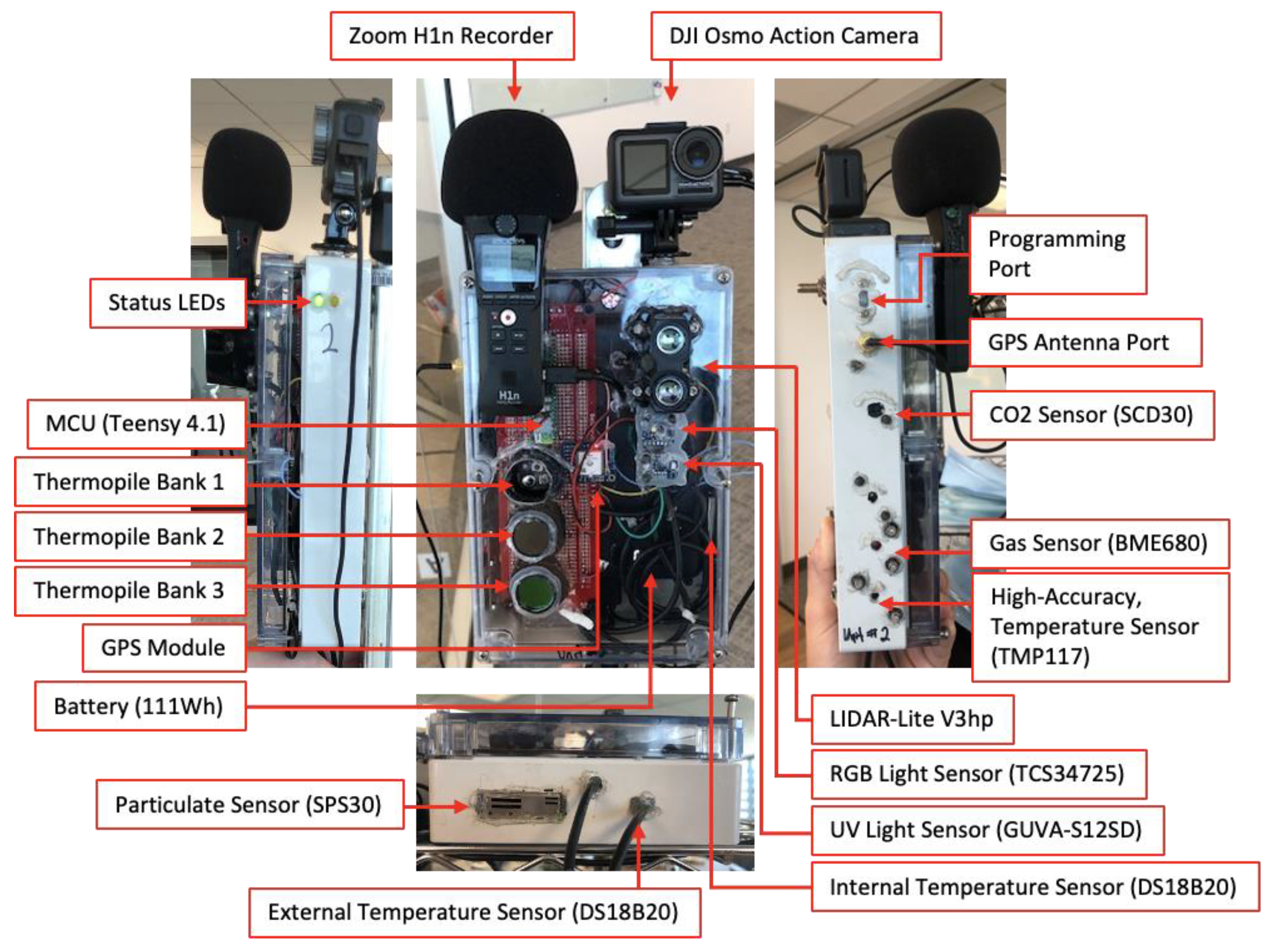
2.1. System Overview

When designing our system, we built around several key constraints to guarantee the operation of our experimental system for a 2-day controlled burn. We derived these constraints from knowing that the unit was going to be placed in remote areas that may be inaccessible until after the experiment and that the fire was going to occur at varying distances near the sensors including directly below. We were also informed by the fire department that the scheduling of the controlled burn may be subject to change, even at the last minute, and that we should be prepared to quickly install and uninstall our systems. The constraints around which we built our system were:
-
Autonomous operation over 48-h;
-
Weather resistant;
-
Continuous camera snapshots for data ground truth over the entire experiment,
-
Installation time less than 10-min so as to not impede the controlled burn training exercises. In an actual deployment for uncontrolled wildfire detection, this would not be a constraint;
-
Local data storage with every sample being timestamped;
-
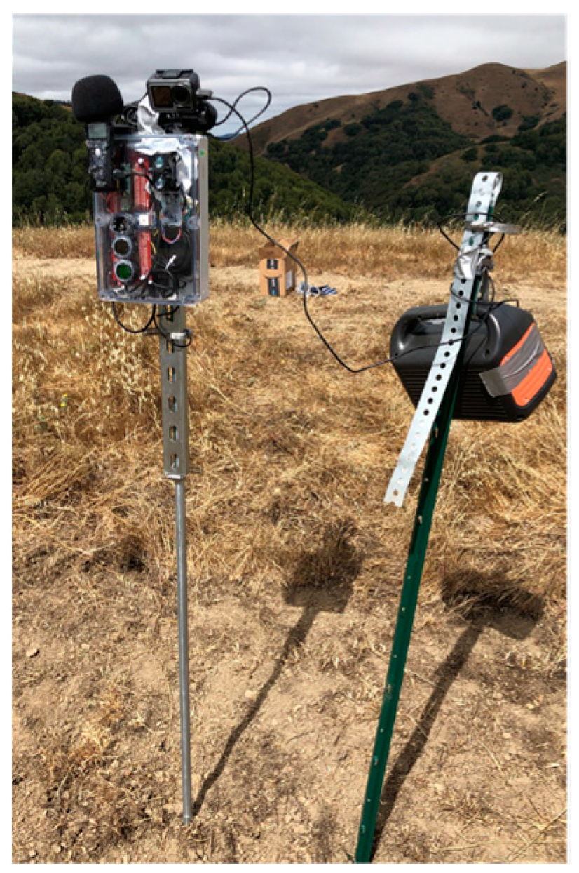
System offset from the ground level to minimize fire risk;
-
Two systems built and deployed simultaneously at different locations to account for the uncertainty of when a controlled burn at a given site will begin and if it will be canceled due to weather or scheduling reasons.
With these constraints in mind, we built two identical versions of the system shown in Figure 1. The system included several COTS sensor modules that were interfaced with an ARM Cortex-M7 MCU (Teensy 4.1). We used several types of temperature sensors to measure the variability across them and the difference between mounting techniques (i.e., external vs. internal). We included a particulate sensor (SPS30), RGB light sensor (TCS34725), UV light sensor (GUVA-S12SD), gas and humidity sensor (BME680), and a CO2 sensor (SCD30). We also added a laser range finder (LIDAR-Lite V3hp) to see whether NIR reflectance in thick smoke could be observed. The system was equipped with an external Zoom H1n microphone and as a truth source, a DJI Osmo Action camera. Two LEDs were added where one was actuated if an error occurred at system startup and another every 1 Hz so that the observer could quickly validate if the sensor unit was operating correctly. All sensor data were recorded to onboard SD cards, a risky decision given that the sensor modules could have been destroyed and all the data would then be lost, but external communication to the device was prohibitive given the complex topography of the area and the uncertainty of how far away a communication relay could be placed. The onboard GPS module was used to periodically synchronize the system with GPS time and limit any clock drift—the antenna was mounted externally to the unit to reduce any signal attenuation from the enclosure. The system was enclosed in a polycarbonate case that was machined to allow for all sensors to have open access to the ambient environment—each sensor had a partial conformal coating with silicone to reduce any risk of water damage.
Our unit was also equipped with nine infrared sensors (i.e., thermopiles) spread over three banks. Bank 1 was exposed to ambient while banks 2 and 3 had additional optical filters. Bank 2 used a bandpass optical filter rated for the CO2 attenuation range (CWL: 4.26 µm, FWHM: 105 nm). Bank 3 used a bandpass optical filter rated near the CO2 attenuation range of 4.3 µm (CWL: 4 µm, FWHM: 500 nm) but the tails of the response curve overlapped with 4.3 µm. Each bank of thermopiles comprised of three discrete digital thermopiles: TSD305, TPiS 1T 1084, and TPiS 1T 1086 L5.5. Digital thermopiles were chosen since the radiation reading compensates for any thermal fluctuations for the sensor itself. TSD305 and TPiS 1T 1084 are equipped with long wave pass filters (attenuation under 5.5 µm) while the TPiS 1T 1086 L5.5 just has a raw silicon lens. Since two of the thermopiles have long wave pass filters that attenuate under 5.5 µm, they cannot measure the ambient atmosphere through either of the bandpass optical filters used in banks 2 and 3 since they attenuate anything above 5.5 µm—this was intentional with the TSD305 but we only learned through a conversation with the manufacturer after the experiment that the TPiS 1T 1084 was also equipped with a similar filter (this detail was omitted from the part’s datasheet). Given the lack of visibility in their responsive regions, these sensors were only able to sense the radiation emitted by the temperature fluctuations of the bandpass lenses themselves.
We maximized the sample rates for each sensor channel by characterizing the sample times required and splitting the digital sensors across all available digital communication peripherals (i.e., three I2C busses, one SPI bus, and the Serial bus) so that each bus only has at most one sensor that requires a lengthy bidirectional communication cycle (>50 ms) for each sample. These sample rates are shown in Table 1. This limits the amount of time the system is deadlocked, waiting for the next available sample, and also reduces the risk of complete system failure in the event that one of the communication busses becomes damaged.
When the sensing system was fully operational, the power draw combined with the recorder operating at 44.1 kHz, was on average 1.53 W, so to fit the requirement of 48-h of autonomous operation, we equipped the unit with a 111 Wh battery, allowing for over 65 h of continuous use on a single charge. We learned that for a 1 Hz sampling rate of the DJI Osmo Action camera, there would be an additional 3.33 W power draw, which warranted a larger/additional battery reserve to keep the unit alive for 48 h. Given that we could not fit a battery large enough within the enclosure to support the camera, we attached an external second power source (240 Wh) dedicated only to the camera’s operation.

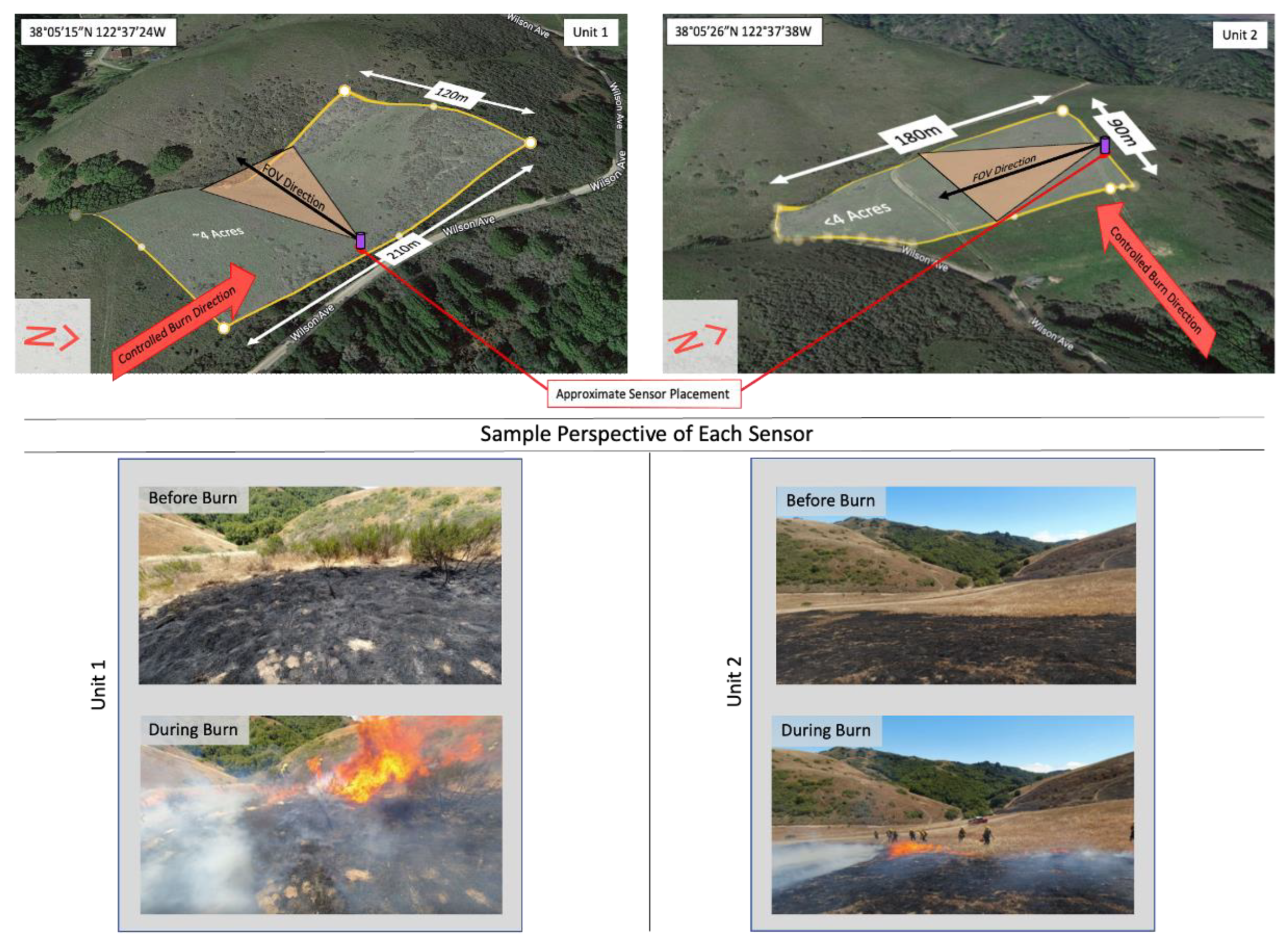
2.2. Experimental Procedure
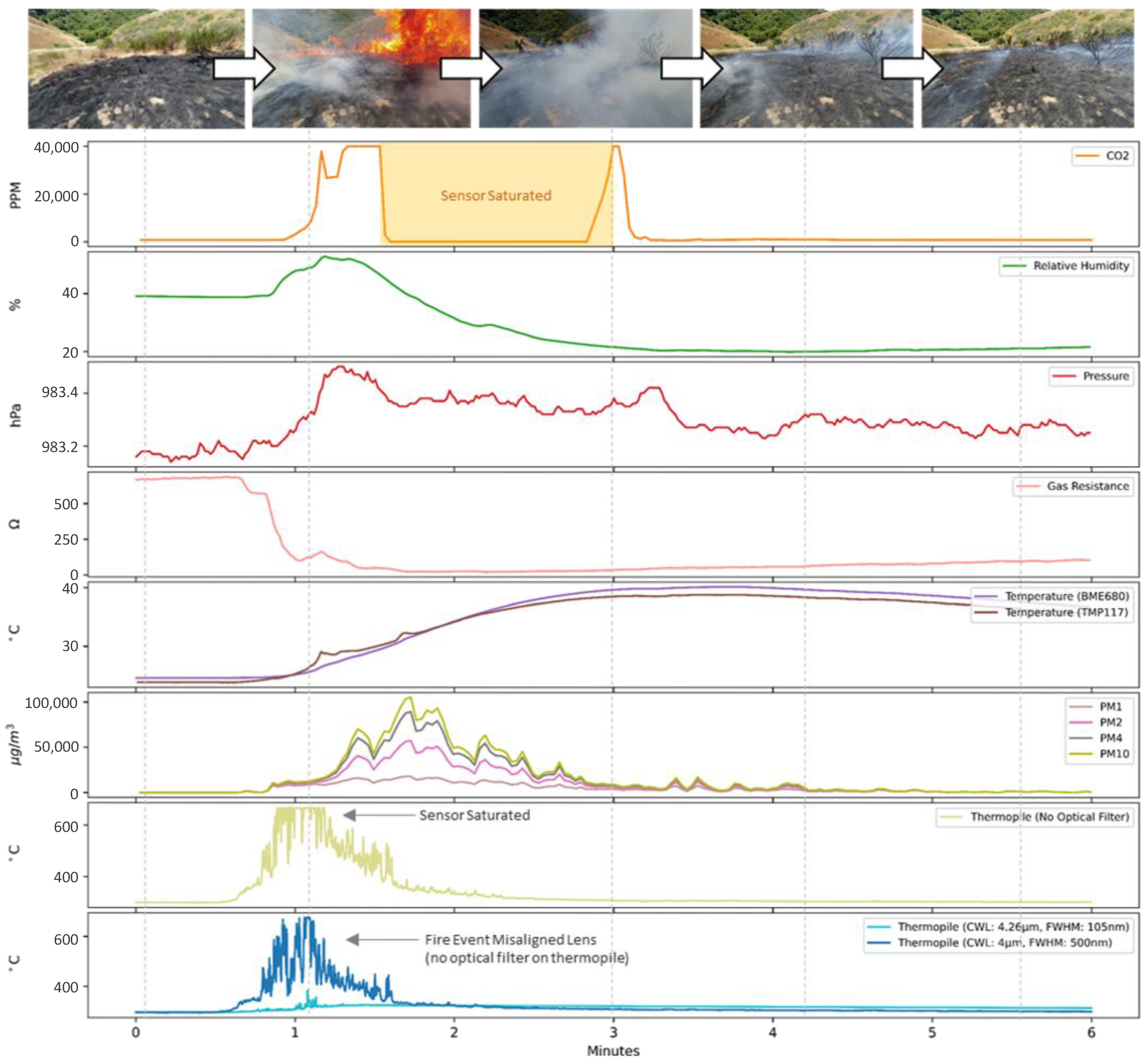
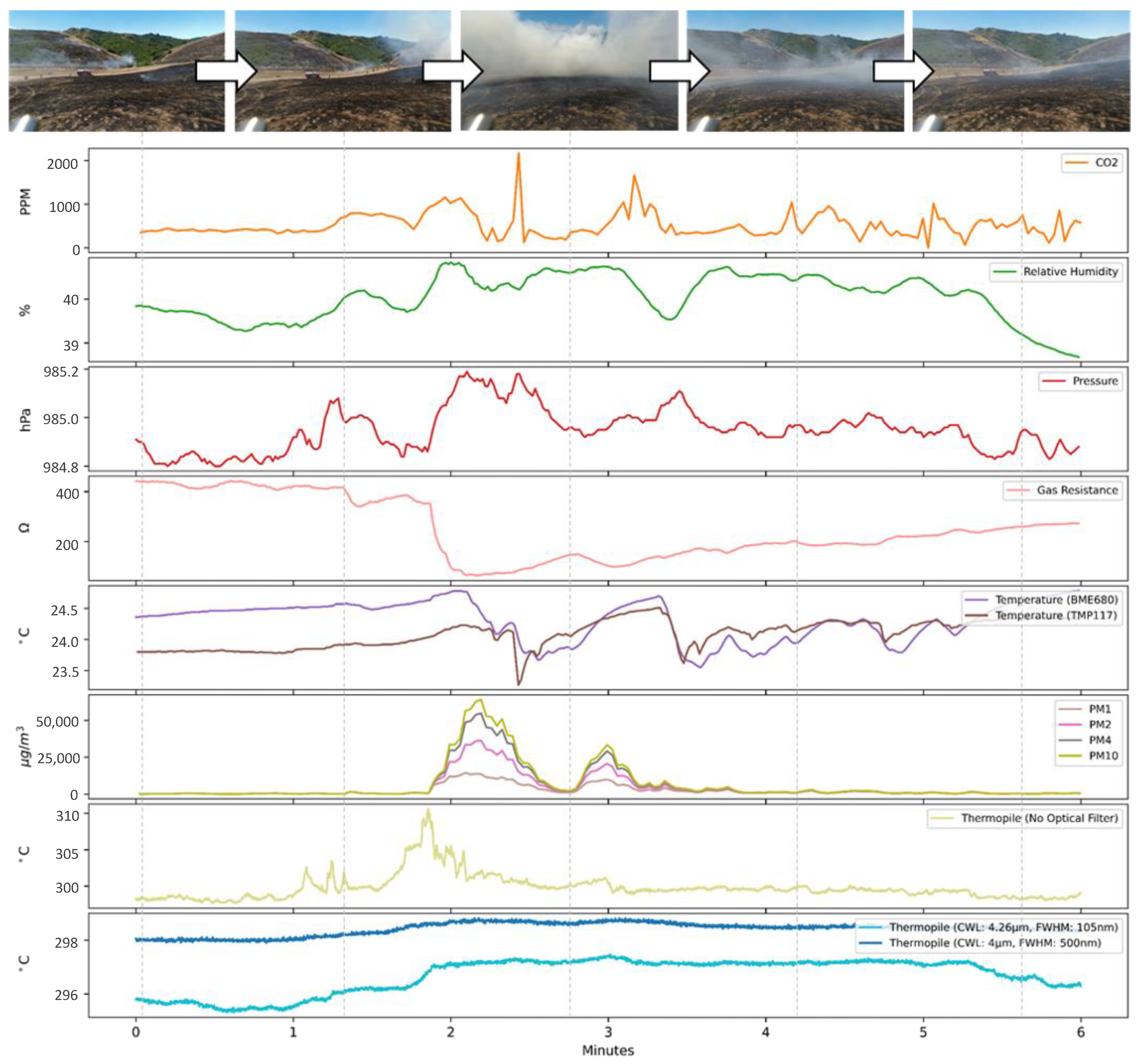
The experiment took place at a controlled burn scheduled by the Marin County Fire Department in Novato, CA. The controlled burn occurred on a large plot of private land where over 80 firefighters continuously burned and extinguished long strips of vegetated land after preparing the land with firebreaks to avoid any unwanted spread. This exercise was used both as a training exercise and as a mitigation technique by burning existing dried vegetation that was at high risk of catching fire.
Our two units were deployed at two different locations across the controlled burn area (Figure 2). Our first unit (Unit 1) was placed in a mixed vegetation area (e.g., tall grass, bushes, etc.) where we expected some of the most intense burns of the event to occur (Figure 3). The second unit (Unit 2) was placed on a hill near the base camp where lower intensity burns were expected, since the only vegetation in the area were fields of short, dry grass. Each sensor unit was placed on 6-foot metal rods with the external batteries places on a second set of rods alongside the sensors to limit direct fire exposure. Unit 2 was installed and left unmoved during the 2-day test event while Unit 1 had to be repositioned twice during the test given that the fire department’s controlled burn plan changed during the experiment and it would not have been able to directly observe a fire in its first location. We were fortunate enough to work with a crew of firefighters on repositioning the sensor twice so that it was less than 5 m downwind from two high-intensity burns (Figure 4).
Figure 5 shows a simplified diagram of the configuration in which each unit was placed. During this controlled burn, an initial firebreak was cut into the landscape, and then firefighters progressed from that break by burning parallel strips of land that ranged in width (i.e., Y meters in Figure 5) but it was observed to be generally around 1–5 m. During each pass, if the firefighters observed that the vegetation was burning too vigorously, they reduced the width of the proceeding strip. The strips were oriented so that the wind naturally blew the fire toward the firebreak to prevent the fire from spreading toward uncontrolled locations. Given this controlled burn test architecture, we placed all of our sensors near the fire break to not impede the firefighting effort and to ensure downwind fire exposure. The exact path and length of land (i.e., X meters in Figure 5) that was burned during each pass was variable and depended on the topography of the landscape. What was also uncertain was when each pass would occur, given that this was dependent on a variety of parameters (e.g., reset time from last pass exercise, water availability, crew readiness, etc.).

3. Results

Over the course of the experiment, both units observed several direct fire events (Table 2). Unit 1 observed two direct fire events at about 5 m while Unit 2 observed several events over the course of two days where they varied in range (directly below the sensor to >30 m away) and intensity. As mentioned in Section 3.2, Unit 1’s placement was moved twice during the experiment, both times being placed in areas that had previously been burned within the past 30 min and in close proximity to the next incoming fire. For all test events, the wind was observed to be blowing from the fire toward the sensors, so direct smoke exposure was true across all cases.
To synchronize all of the sensor data, the environmental sensors were synchronized with the onboard microcontroller’s running clock and also with GPS time to compensate for clock drift. For the DJI Action Camera, the video frames proved to be difficult to automatically synchronize with the rest of the system. The first attempt at time synchronizing the camera frames with the sensor data started with summing the pixel values of each frame, making a signal out of this sum by doing this for all frames, and then comparing this signal to the RGB light sensor on the sensor unit. A cross-correlation was performed and the initial attempts looked promising, but when validating the fire events seen by the CO2 signal with the corresponding synchronized camera frame, it appeared to be misaligned by several minutes. The main reason for misalignment was that the camera had a very active automatic gain control (AGC) that made cross-correlating with the RGB light sensor difficult. We settled on cross-correlating over a region of time that the AGC was stable (consistent lighting in the scene); this allowed us to manually fine-tune the alignment. We also noticed that although the camera was supposed to be recording at 1 Hz, it was slightly off, resulting in increased misalignment as the video progressed from where we fine-tuned it. To compensate, we recalculated the alignment for each new day of testing. With the frames synchronized, we generated several video snippets for each test event where we showed the temporal evolution of each sensor channel mapped to the camera frames so that it could inform our qualitative analysis; a link to the video snippets can be found here: https://tinyurl.com/ynuhuha7 (accessed on 8 June 2022). We did not include the microphone data for this phase of analysis, but it will be a focus in our future work. We also did not include the laser range finder data since the results were inconclusive. Theoretically, we should be able to sense smoke-related reflectance in the NIR band using a NIR laser-based ToF sensor; the sensor we used preprocessed the raw signal and only returned the estimated distance of the maximum reflectance point.
For two of the 12 fire events seen by our two sensors (Table 2), the raw signals of a subset of our sensors are shown in Figure 6 and Figure 7. Figure 6 is the first event seen by Unit 1 that was exposed to a nearby high-intensity fire. Figure 7 is the last event seen by Unit 2 where the controlled burn occurred over 20 m away. Both figures feature a few snapshots from each unit’s cameras to provide a visual frame of reference. It is important to note that throughout both testing days, the entire test event area had an increase in smoke activity given the multiple controlled burns occurring on various hills in the vicinity.

3.1. Temperature, Humidity, and Pressure

For the multiple modes of temperature sensing we had on the unit, all sensors saw a momentary increase during each fire event. We chose to present a subset of results in this paper since the other temperature sensors yielded similar temperature ranges and the responsivity across all internal sensors was similar, although the externally mounted sensor was the quickest to respond given its ability to make direct contact with the hot smoke. However, upon request, we can make the full data collection available. For the closest of the fires observed (Unit 1: event 1, Figure 6), we saw temperature fluctuations of 15 °C while for the furthest of events (Unit 2: event 10, Figure 7), we were still able to observe a near 1 °C momentary rise. However, during the furthest of the fire events seen during testing, the temperature fluctuations were minimal and virtually nonexistent in the cheapest and lowest resolution temperature sensors (e.g., DS18B20). Our units benefitted from having direct contact with the hot smoke being blown over it, so that had a strong influence on the system’s quick response after ignition. For the pressure fluctuation, we observed significant variability across the entire experiment, likely caused by the convective nature of the fire itself, but the results are inconclusive given that the strong wind currents in the area are a dominating factor when measuring the pressure fluctuations of the environment.
During ignition and a short time right after, we saw sharp increases in humidity (e.g., Figure 6) as any existing moisture in the ground evaporated and was carried downwind toward the sensor. We did not observe these sharp increases when the fire was ignited directly below the sensor (<1 m radius) since the moisture was blown away by the air currents. Similarly, when the fire was ignited at its furthest (>20 m), the humid exhaust diffused, which resulted in a highly dynamic signal.

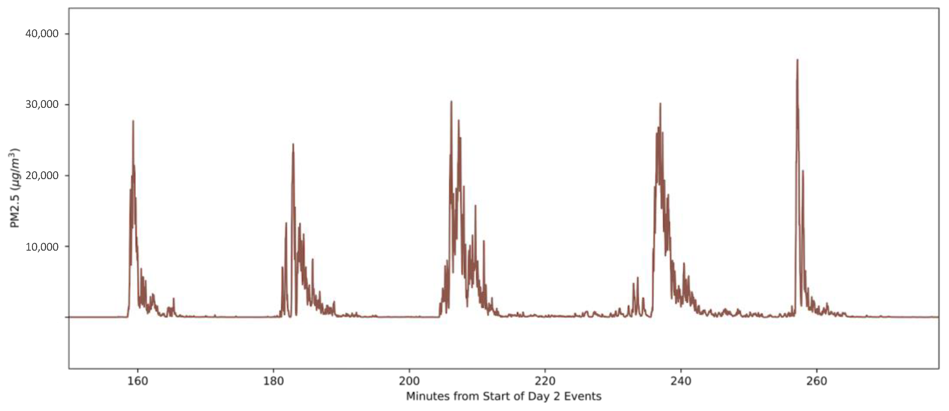
3.2. Particulate Matter
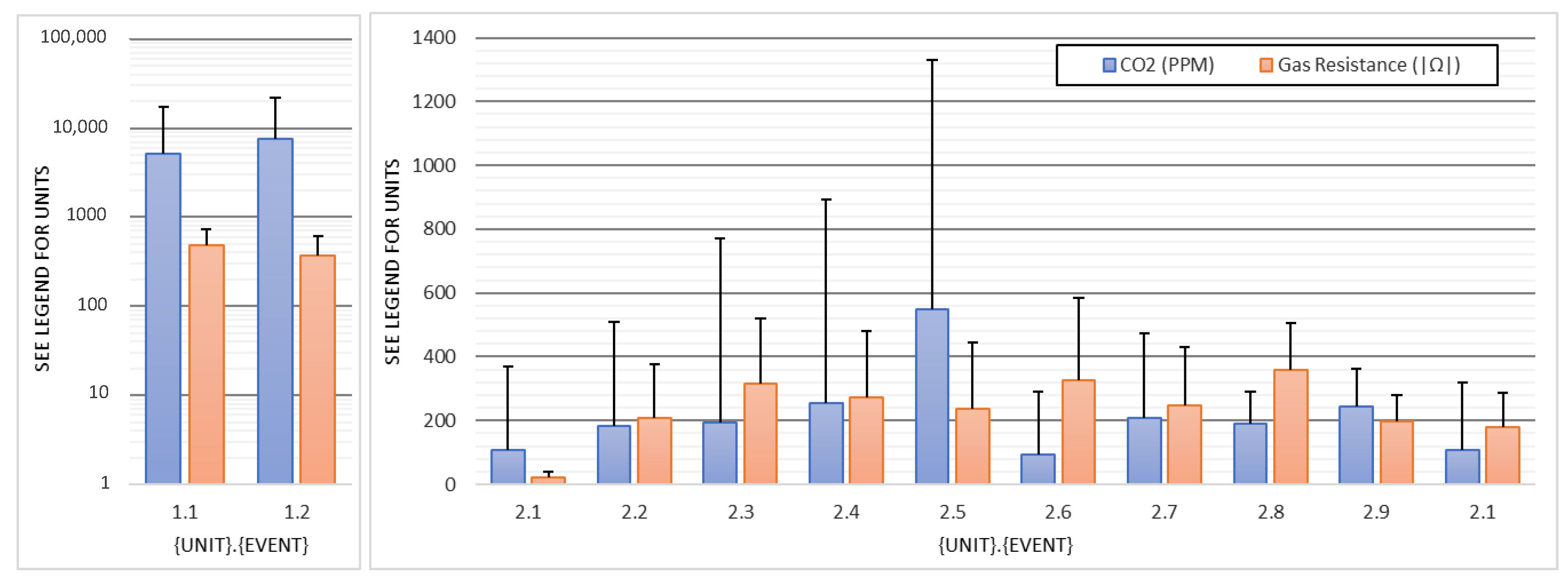
We took the difference of a 4-min average particulate count directly prior and during each fire event (Figure 8). For Unit 2, events 8–10, the test area started to become noticeably hazy due to the ongoing controlled burns upwind from the test site, which is why the particulate count prior to those fire events was higher than the previous events. As can be seen in Figure 8, the particulate count across PM 1, PM 2.5, PM 4, and PM 10 rose sharply during all fire events—these measurements continued to linger at above-average levels for several minutes after, as the ground continued to smolder. Figure 9 shows how abrupt the unfiltered signal looked for the PM 2.5 mass concentration measurements across five sequential controlled burns. The smallest particulate count response was seen during Unit 2’s first fire event, where the fire occurred directly below the device and the wind was able to effectively push the particulate matter away from the sensor. These results clearly show that the particulate count is strongly dependent on wind direction and sensor placement.
We did not see an appreciable relationship between particulate count and distance between the sensor and the fire. No significant concentration differences were seen when the sensor unit was exposed to a fire event at 5 m (Unit 2: event 3) or to a fire in excess of 20 m away (Unit 2: event 10). This was likely due to the strong wind currents observed that day, so further testing is required to estimate how much the particulates diffuse for a given air current and distance. We did see that the particulate count is dependent on the concentration of fuel being burned near the devices, since Unit 1’s first event (Figure 6) had roughly double the concentration of PM observed when compared to its second event, which is likely due to a large bush that ignited directly in front of our device, resulting in a greater measured density of particulate discharge.

3.3. Gas

Similar to the particulate count measurements, the CO2 PPM saw a dramatic increase in measurements and signal volatility during the fire but, unlike the PM count, quickly returned to pre-event CO2 concentrations once the fire was extinguished (Figure 10). The signal was also far noisier than the PM count, likely due to the variable air currents and continued fire activity throughout the region. For Unit 1, the CO2 sensor saturated to its max count (40,000 PPM) for both high-intensity fire events. We realized that once the sensor saturated, the reading dropped to zero while the sensor underwent an internal reset process, as seen in Figure 6. To compensate, we removed the zero values and forward-filled the values when calculating the average differences shown in Figure 10.
The gas resistance output by BME680 is the resistance across the metal oxide sensor, which drops when it encounters specific types of gas such as volatile organic compounds (VOCs). The exact value cannot be mapped to a specific level of VOCs without proper calibration; Bosch calibrated these sensors to map the gas resistance to air quality, equivalent-CO2, and other metrics, but they only pertain to indoor applications. The gas resistance during each event phase saw dramatic dips in the averages while dramatic increases in volatility during the burn with lingering effects were seen for some time after the burn, unlike the CO2 sensor readings. This is likely due to BME680 being sensitive to a wide array of exhausting gases that are still present several minutes after the burn, unlike CO2. which appears to dissipate relatively quickly.

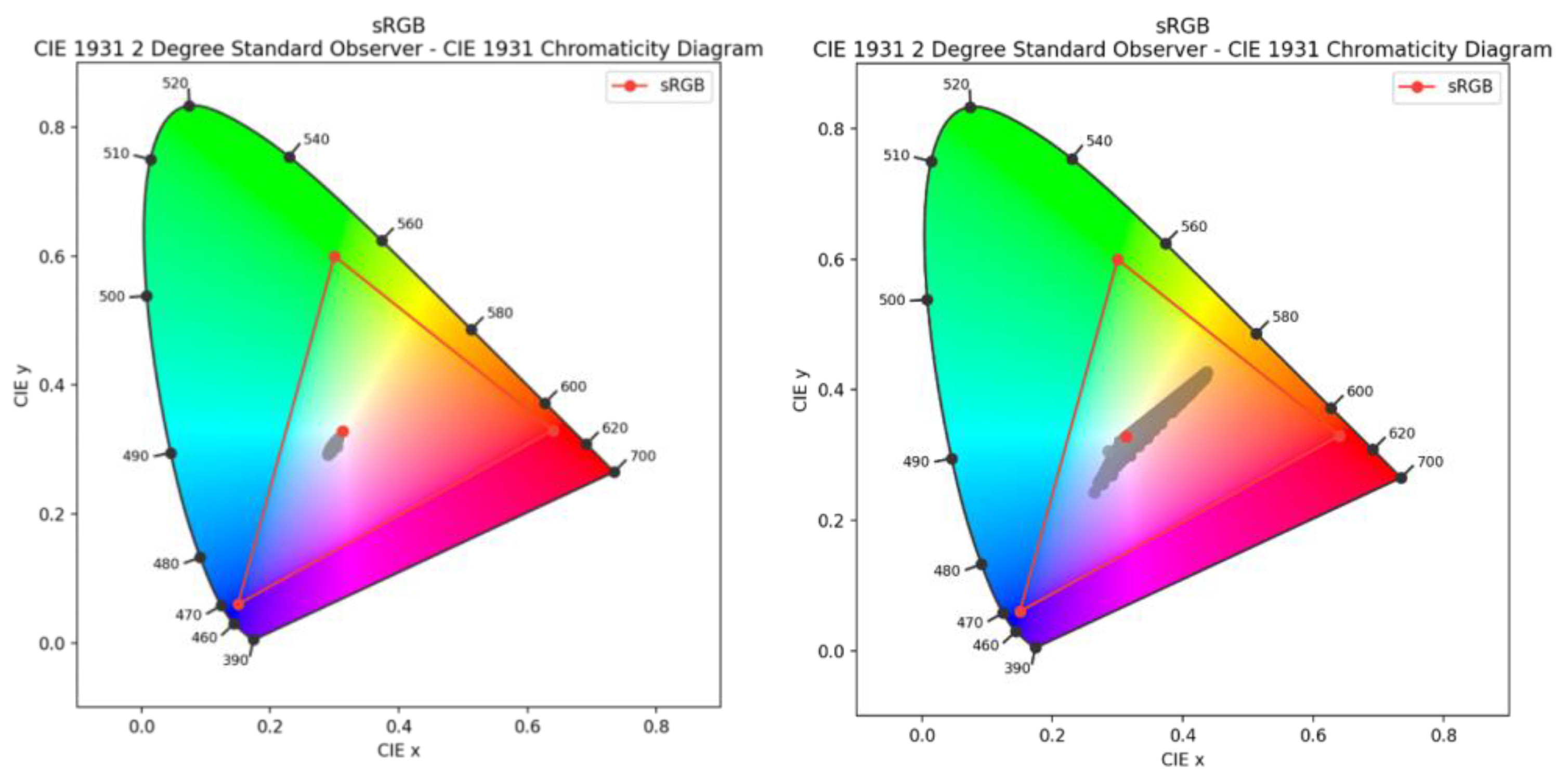
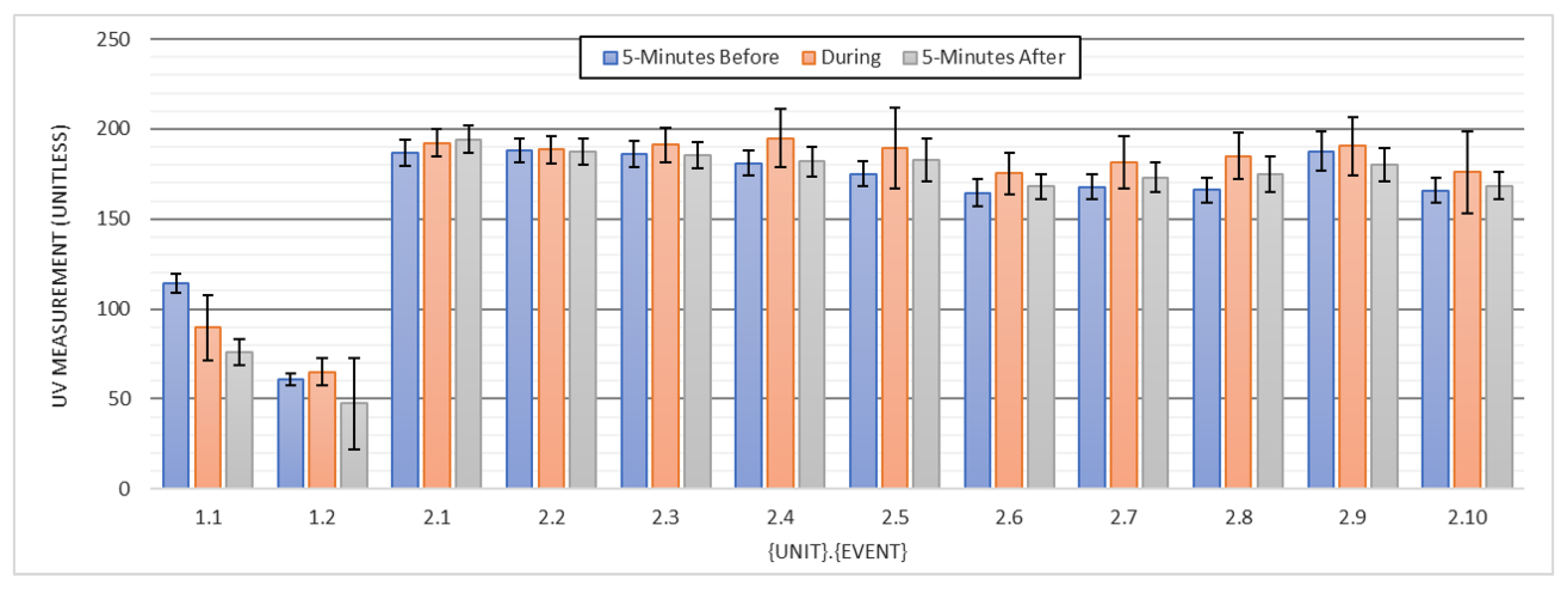
3.4. Optical: Visible and UV

We split the RGB sensor values measured during each fire event and plotted them next to the remaining measurements (Figure 11); the data are a combination of both sensor units (Unit 1 and Unit 2) and span 2 full days and a night. It is clear that the in-event measurements are a subset of the out-of-event measurements and cannot be used alone to classify a fire event. Nonetheless, the smoke has a specific color profile (Figure 11, left) that can be used in daylit scenarios to increase the confidence of a fire detection sensing system. Although it appears that the out-of-event measurements also include similar RGB values as the in-event measurements, it is important to note that even during times where there was not a fire present in the immediate vicinity, the area was still hazy from the other controlled burns happening in the area. Further work is warranted on collecting more measurements from clean events and comparing them to the near-fire data.
In Figure 12, we calculated the mean of the UV data 4-min before and after each event and compared to that of the mean during (4-min windows). For Unit 1, we expected to see a significant increase in UV for both test events given the close proximity the unit was to high-intensity burns. We did see momentary spikes in the data but the average UV measurement during the burn was less than or comparable to the measurements directly prior. We believe this is because, after the initial ignition where a large fire enveloped the sensor, the fire quickly subsided and was out of the FOV of the optical UV sensor. With the increased wind activity, the sensor had no visibility to the fire or the exhaust after the initial ignition. For Unit 2, we saw similar results, but as the fire events grew in distance from the sensor, we saw a greater disparity between the measurements during and before the fire. We expected reduced UV activity in the presence of smoke since the smoke particulates occluded UV exposure from the Sun and ongoing fires, but it appears that we were still able to detect minor increased levels of UV radiation. Although the initial results look promising, further validation is required in more controlled experiments where we can limit the amount of particulate exhaust and the intensity of the burn. We were also limited by the type of UV sensor we could use that offered uncalibrated, unitless measurements.

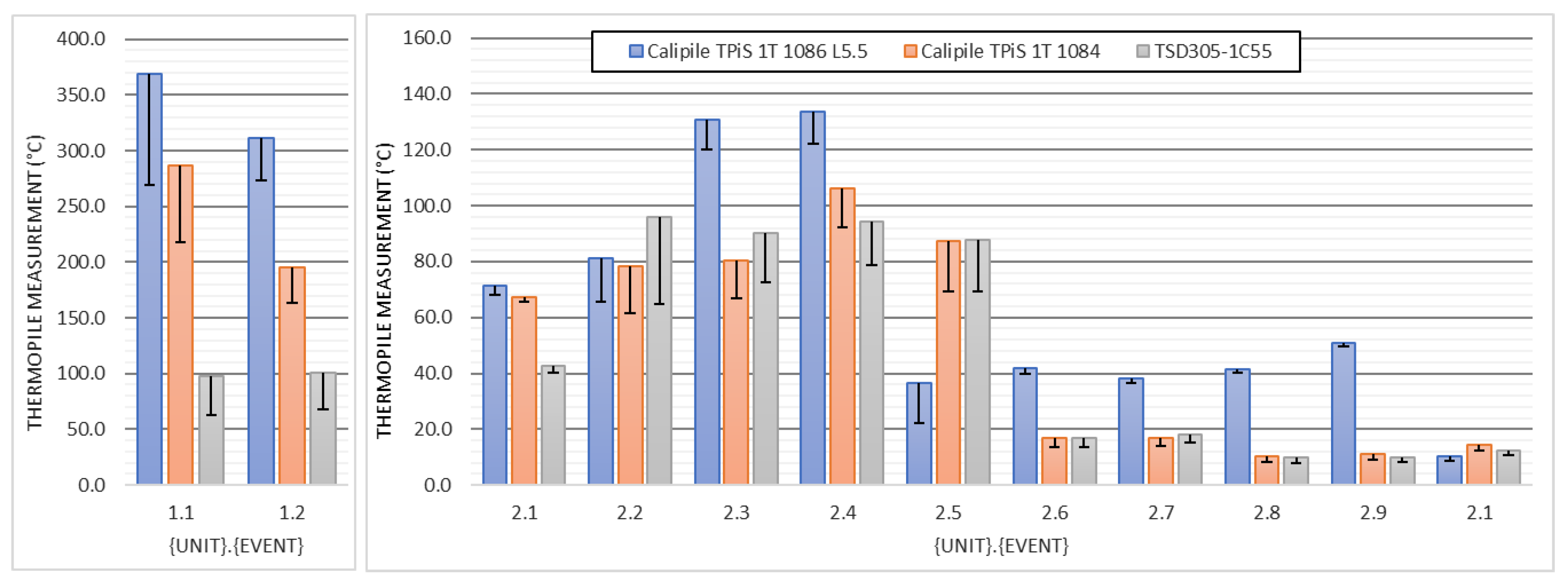
3.5. Optical: Infrared

Figure 13 shows the data from the bank 1 thermopiles, which had no additional optical filtering besides the ones they were equipped with from the factory. For the analysis, we looked at the max temperature fluctuations observed within a 4-min window directly before and during the fire while also taking into consideration the standard deviation of the samples within that window. In Figure 13, we show the differences between these two maximums to prove the feasibility of using these sensors as wildfire detectors. These thermopile measurements were adjusted/normalized to fluctuating changes in the thermopile housing temperatures. To compensate, we used the manufacturer’s built-in calibration constants for each sensor and applied them in real-time. Figure 6 and Figure 7 show the raw signals from the TpiS 1T 1084 L5.5 thermopile across the optical banks.
Unsurprisingly, the greatest infrared fluctuations that we saw were those with the most intense burns (Unit 1: events 1 and 2). For Unit 2, as the fire events grew in distance from the sensor, the temperature readings and variability in the readings decreased. The hot smoke diffused through the air, which led to a more uniform temperature profile. When the fire was right below the sensor (Unit 2: event 1), the thermopiles picked up on the increased temperature but the standard deviation across the window remained low. We believe that this is because the thermopile was not exposed to the hot smoke as it was blown away from its FOV, but did observe a transient flame or hot smoke trail, which led to the sudden but short spike. The performance across the thermopiles with similar FOVs (i.e., TSD305 and TpiS 1T 1084) was virtually the same, but the TpiS 1T 1086 thermopile with the tighter FOV (5° vs. 60°) had a stronger response throughout, especially for events where the fire was far away from the sensor (Unit 2: events 6–10). The performance differences are because the wider FOV thermopiles trade-off responsivity for increased visibility, which is great when looking at a large scene and only looking for a significant change from the steady-state. The wider FOV thermopiles had an increased standard deviation during further fire events (Unit 2: events 4–10) from that of the narrower FOV thermopile since they were responding to all of the thermal activity occurring within their visibility region while the narrower-FOV thermopile saw spurious peaks when hot smoke or a flame trail crossed its optical path. However, when specifically looking for a fire event down a narrow corridor (i.e., down a long, narrow clearing), a better performance will be obtained from a narrower FOV sensor since it only captures the area of interest.
As for the thermopile data in the other banks, the results are inconclusive since we observed sudden temperature fluctuations during each test event on the thermopiles that were supposed to have an optically opaque FOV (TSD305 and TpiS 1T 1084), preventing them from direct observation of the fire events. We believe that the cause of this phenomenon is because since we were downwind from each fire, the optics in banks 2 and 3 heated up via convection from the hot smoke, resulting in increased thermal radiation at the bands the thermopiles were sensitive. So, although the thermopiles could not observe the fire directly, they were able to visualize their effects through a proxy. We did observe that the optical filters were attenuating a significant portion of the infrared when one of the two filters was forced out of place due to the extreme fire exhaust during Unit 1’s first fire event (Figure 6). The difference between the signals of the two filtered thermopiles was far greater for Unit 1’s first event, where one of the filtered sensors was uncovered, than that observed in other experiments such as the one shown in Figure 7. Further experimentation is required in other configurations where the heat from the fire does not make direct contact with the sensing unit.

4. Discussion

4.1. Multimodal Sensing Approach for Fire Detection

This experiment demonstrated the capabilities of several different sensing modalities on detecting a fire event under specific parameters (e.g., illuminated scene, downwind, and no visual obstruction from the sensor to fire). The RGB light sensor showed promise in detecting the color signature of smoke, but that was not enough to confidently classify a fire event. It would not work in dark conditions and the color profile is a subset of possible color profiles in non-smoke events. Similarly, the UV sensor saw significant disturbances in the UV measurements during a fire event, but this can also occur in nature due to intermittent sunlight from the swaying of foliage. The thermopiles accurately detected fire events, only under the condition that the fire event was within their FOV. We did not test the thermopiles in upwind conditions where the convective heating from the smoke would not influence the signal. Particulate and gas sensors demonstrated strong responses to fire events, especially where direct visibility was lacking, but these sensors require direct contact with the fire’s exhaust, which may be unlikely due to wind patterns. This requirement can be resolved through distributed sensing but may be cost-prohibitive.
It is clear from this study that a robust fire detection system using one sensing modality is simply not possible when taking into consideration the dynamics of natural environments and the feasibility of a densely distributed network in the wild. A system could be placed in a dense mesh across a landscape, but the cost of manufacturing, installation, and maintenance may be prohibitive. A more cost-effective approach may be to sparsely distribute sensors that are equipped with multiple sensing modalities and can communicate with each other to operate in concert. Not only could a fire be classified in proximity to each sensor, but by using differential measurements across units (e.g., significant variance in particulate and gas concentrations), a distributed system can be used to estimate the locations and size of the fires. With such a sparsely distributed multi-sensor system, the degree of wildfire spread could also potentially be detected and modeled using the relationships of fire to the local humidity and wind dynamics.

4.2. Practical Considerations

Several of the most substantial constraints in creating a distributed fire detection system are the cost and deployment feasibility, metrics that were not thoroughly evaluated in this study but will be evaluated in the context of our future work. In principle, we can integrate each sensor we used in this study into a comprehensive sensing unit, fit it with a large solar panel, and deploy it in mass across a large landscape that is vulnerable to a wildfire. Although possible, this type of system would not be ideal for any municipality to deploy, both because of the financial costs and esthetic reasons—people may not want large electronic units scattered across their public areas. We suggest that an affordable and effective mesh-based fire detection sensor system could balance several factors: (1) optimal sensing diversity to detect a wildfire event accurately and quickly, (2) cost and visible footprint, and (3) additional landscape-wide sensing services that may be of value to land managers and owners. For the sensing diversity question, more data need to be collected in naturalistic environments to properly characterize the accuracy and repeatability of sensors in detecting fires. Long-term studies are also required to assess the practical sensor considerations of outdoor deployments into remote regions. Apart from fire detection, there is a wealth of knowledge that a distributed sensing system provides, especially in areas rich with microclimates. Having physical sensing nodes scattered across a landscape offers direct insight into environmental parameters that are tough to measure indirectly. The argument for a distributed system strengthens when pursuing a multi-faceted classification approach where the data can be made public for others to use in understanding varying parameters across large areas that inform environmental public policies (e.g., where there is increased air pollution trending, monitoring noise levels of human activity, etc.).

5. Conclusions

Wildfires are becoming an increasing threat to communities, livelihoods, and ecosystems around the world. As our climate changes, causing drought conditions and volatile weather patterns, the continual increase in the probability of annual destructive wildfires raises alarms for residential communities that are at high risk of exposure to direct fires or their pollutants. Given that fires can begin in isolated areas with limited human presence and difficult terrain to navigate, there is a strong case for automated distributed fire detection capabilities to limit the spread and potential destruction of such fires. In our work, we presented several potential fire sensing modalities, integrated them into custom datalogging units, and collected and analyzed data from a 2-day controlled burn. Given the experimental conditions, nearly all sensing modalities exhibited signature behaviors when exposed to active flames and their exhaust, but with varying degrees of sensitivity. Further work is warranted to fully assess the practicality of each sensor for long-term outdoor applications, but with these results, it is clear that any fire detection system requires a multi-modal sensing approach for robust and accurate detection.
For future work, we plan on collecting more sensor data at other controlled burns where we can diversify the positioning of our devices such as placing them upwind from the fire, therefore preventing our system from experiencing any direct contact with the exhausted particulates and gases. This will allow us to thoroughly test our various thermal optical sensors and avoid any signal disturbances from self-heating. This will also allow us to understand the failure modes of our particulate and CO2 sensors, which require direct exposure to the exhausted material. In addition to working with fire departments on control burns, we seek to create more controlled lab experiments where we can test how our sensors perform when we artificially vary the materials being burnt, the amount of smoke exhausted from incomplete combustion, and how well our optical sensors perform during nighttime use. On a system design front, additional work is needed to understand how these systems should be powered, how long they will last in the wild, how they will communicate from remote regions with potentially poor network connectivity, and the cost and deployment feasibility. The promising results of this study suggest that these additional efforts are warranted.

Author Contributions

Conceptualization and writing of the manuscript, T.A., J.D., P.C. and H.C.; Data and analysis of figures and tables, P.C., H.C. and P.D.; Writing of manuscript, J.D., T.A., S.S., C.C. and P.C. All authors have read and agreed to the published version of the manuscript.

Funding

This research received no external funding.

Institutional Review Board Statement

Not applicable.

Informed Consent Statement

Not applicable.

Data Availability Statement

All data used in this research are publicly available.

Conflicts of Interest

The authors declare no conflict of interest.

References

  1. Bump, P. Analysis—Six of California’s Seven Largest Wildfires Have Erupted in the Past Year. Washington Post. 2021. Available online: www.washingtonpost.com/politics/2021/08/06/six-californias-seven-largest-wildfires-have-erupted-past-year/ (accessed on 11 August 2021).
  2. Reyes-Velarde, A. California’s Camp Fire Was the Costliest Global Disaster Last Year, Insurance Report Shows. Los Angeles Times. 2019. Available online: https://www.latimes.com/local/lanow/la-me-ln-camp-fire-insured-losses-20190111-story.html (accessed on 9 September 2023).
  3. U.S. Fire Administration. n.d.; What Is the WUI? Available online: www.usfa.fema.gov/wui/what-is-the-wui.html (accessed on 11 August 2021).
  4. Blalack, T.; Ellis, D.; Long, M.; Brown, C.; Kemp, R.; Khan, M. Low-Power Distributed Sensor Network for Wildfire Detection. In Proceedings of the 2019 SoutheastCon, Huntsville, AL, USA, 11–14 April 2019; pp. 1–3. [Google Scholar]
  5. PurpleAir: PurpleAir Map, Air Quality Map. Available online: http://map.purpleair.org/ (accessed on 1 August 2019).
  6. Saldamli, G.; Deshpande, S.; Jawalekar, K.; Gholap, P.; Tawalbeh, L.; Ertaul, L. Wildfire Detection using Wireless Mesh Network. In Proceedings of the 2019 Fourth International Conference on Fog and Mobile Edge Computing (FMEC), Rome, Italy, 10–13 June 2019; pp. 229–234. [Google Scholar]
  7. Cui, F. Deployment and integration of smart sensors with IoT devices detecting fire disasters in huge forest environment. Comput. Commun. 2020, 150, 818–827. [Google Scholar] [CrossRef]
  8. Hidestal, C.; Zreik, A. Smart Environment Early Wildfire Detection Using IoT. Master’s Thesis, Lund University, Lund, Sweden, 2020. [Google Scholar]
  9. Rizanov, S.; Stoynova, A.; Todorov, D. Single-Pixel Optoelectronic IR Detectors in Wireless Wildfire Detection Systems. In Proceedings of the 2020 43rd International Spring Seminar on Electronics Technology (ISSE), Demanovska Valley, Slovakia, 14–15 May 2020; pp. 1–6. [Google Scholar]
  10. U.S. National Park Service. Wildland Fire: What is a Prescribed Fire? Available online: www.nps.gov/articles/what-is-a-prescribed-fire.htm (accessed on 11 August 2021).
  11. Yuan, C.; Zhang, Y.; Liu, Z. A survey on technologies for automatic forest fire monitoring, detection, and fighting using unmanned aerial vehicles and remote sensing techniques. Can. J. For. Res. 2015, 45, 783–792. [Google Scholar] [CrossRef]
  12. Ankita, M.; Trinh, T. Early Wildfire Detection Technologies in Practice—A Review. Sustainability 2022, 14, 12270. [Google Scholar] [CrossRef]
  13. Allison, R.; Johnston, J.; Craig, G.; Jennings, S. Airborne Optical and Thermal Remote Sensing for Wildfire Detection and Monitoring. Sensors 2016, 16, 1310. [Google Scholar] [CrossRef]
  14. Gunay, O.; Tasdemir, K.; Toreyin, B.U.; Cetin, A. Video based wildfire detection at night. Fire Saf. J. 2019, 44, 860–868. [Google Scholar] [CrossRef]
  15. Sittakul, V.; Pasakawee, S.; Jan-im, C. Wireless Sensor Network for Wildfire Detection and Notification via Walkie—Talkie Network. In Proceedings of the 2019 16th International Conference on Electrical Engineering/Electronics, Computer, Telecommunications and Information Technology (ECTI-CON), Pattaya, Thailand, 10–13 July 2019; pp. 673–676. [Google Scholar]
  16. Lindsey FireSense. Available online: https://lindsey-firesense.com/ (accessed on 2 June 2021).
  17. IQ FireWatch. 2021. Available online: https://www.iq-firewatch.com/ (accessed on 2 June 2021).
  18. Lesnoy Dozor: Protects Forest from Fire. n.d. Available online: http://lesdozor.ru/en/ (accessed on 2 June 2021).
  19. FireHawk. 2021. Available online: https://home.firehawk.co.za//home (accessed on 2 June 2021).
  20. Anderson, H.E. Heat Transfer and Fire Spread; Res. Pap. INT-RP-69; Intermountain Forest and Range Experiment Station, Forest Service, U.S. Department of Agriculture: Ogden, UT, USA, 1965; Volume 20, p. 69.
  21. Frankman, D.; Webb, B.W.; Butler, B.W.; Jimenez, D.; Forthofer, J.M.; Sopko, P.; Shannon, K.S.; Hiers, J.K.; Ottmar, R.D. Measurements of convective and radiative heating in wildland fires. Int. J. Wildland Fire 2012, 22, 157–167. [Google Scholar] [CrossRef]
  22. Ulucinar, A.R.; Korpeoglu, I.; Cetin, A. A Wi-Fi Cluster Based Wireless Sensor Network Application and Deployment for Wildfire Detection. Int. J. Distrib. Sens. Netw. 2014, 10, 651957. [Google Scholar] [CrossRef]
  23. Barducci, A.; Guzzi, D.; Marcoionni, P.; Pippi, I. Infrared detection of active fires and burnt areas: Theory and observations. Infrared Phys. Technol. 2002, 43, 119–125. [Google Scholar] [CrossRef]
  24. Ward, D. Chapter 3—Combustion Chemistry and Smoke. In Forest Fires; Johnson, E.A., Miyanishi, K., Eds.; Academic Press: San Diego, CA, USA, 2001; pp. 55–77. [Google Scholar] [CrossRef]
  25. Sun, H.L.; Rong, Z.; Liu, C.; Liu, J.; Zhang, Y.; Zhang, P.; Wang, X.; Gao, W. Spectral characteristics of infrared radiation from forest fires. In Proceedings of SPIE—Remote Sensing and Modeling of Ecosystems for Sustainability III; SPIE: Bellingham, WA, USA, 2006; Volume 6298. [Google Scholar]
  26. Potter, B.E. The role of released moisture in the atmospheric dynamics associated with wildland fires. Int. J. Wildland Fire 2005, 14, 77–84. [Google Scholar] [CrossRef]
  27. Lutakamale, A.S.; Kaijage, S. Wildfire monitoring and detection system using wireless sensor network: A case study of Tanzania. Wirel. Sens. Netw. 2017, 9, 274–289. [Google Scholar] [CrossRef]
  28. Byram, G.M. Combustion of forest fuels. In Forest Fire: Control and Use; Davis, K.P., Ed.; McGraw-Hill: New York, NY, USA, 1959; pp. 61–89. [Google Scholar]
  29. Dampage, U.; Bandaranayake, L.; Wanasinghe, R.; Kottahachchi, K.; Jayasanka, B. Forest fire detection system using wireless sensor networks and machine learning. Sci. Rep. 2022, 12, 46. [Google Scholar] [CrossRef] [PubMed]
  30. Hartung, C.; Han, R.; Seielstad, C.; Holbrook, S. FireWxNet: A multi-tiered portable wireless system for monitoring weather conditions in wildland fire environments. In Proceedings of the 4th International Conference on Mobile Systems, Applications, and Services (MobiSys 2006), Uppsala, Sweden, 19–22 June 2006. [Google Scholar]
  31. National Wildfire Coordinating Group. Belt Weather Kit. 2022. Available online: https://www.nwcg.gov/term/glossary/belt-weather-kit (accessed on 2 June 2021).
  32. Bayo, A.; Antolín, D.; Medrano, N.; Calvo, B.; Celma, S. Development of a wireless sensor network system for early forest fire detection. In Proceedings of the European Workshop on Smart Objects: Systems, Technologies and Applications, Ciudad, Spain, 15–16 June 2010; pp. 1–7. [Google Scholar]
  33. Rothermel, R.C. A Mathematical Model for Predicting Fire Spread in Wildland Fuels; Res. Pap. INT-115; Intermountain Forest and Range Experiment Station, Forest Service, U.S. Department of Agriculture: Ogden, UT, USA, 1972; 40p.
  34. Albini, F.A. Estimating Windspeeds for Predicting Wildland Fire Behavior; Intermountain Forest and Range Experiment Station, Forest Service, U.S. Department of Agriculture: Ogden, UT, USA, 1979; Volume 221.
  35. Wu, J.; Van Vroonhoven, C.; Chae, Y.; Makinwa, K. A 25mW CMOS sensor for wind and temperature measurement. In Proceedings of the SENSORS IEEE, Limerick, Ireland, 28–31 October 2011; pp. 1261–1264. [Google Scholar]
  36. Hays, M.D.; Geron, C.D.; Linna, K.J.; Smith, N.D.; Schauer, J.J. Speciation of Gas-Phase and Fine Particle Emissions from Burning of Foliar Fuels. Environ. Sci. Technol 2002, 36, 2281–2295. [Google Scholar] [CrossRef] [PubMed]
  37. Yadav, I.C.; Devi, N.L. Biomass Burning, Regional Air Quality, and Climate Change. Earth Syst. Environ. Sci. 2019, 386–391. [Google Scholar]
  38. Li, X.; Wang, S.; Duan, L.; Hao, J.; Li, C.; Chen, Y.; Yang, L. Particulate and trace gas emissions from open burning of wheat straw and corn stover in China. Environ. Sci. Technol. 2007, 41, 6052–6058. [Google Scholar] [CrossRef] [PubMed]
  39. National Research Council: Committee on Air Quality Management in the United States, Board on Environmental Studies and Toxicology, Board on Atmospheric Sciences and Climate, Division on Earth and Life Studies. Air Quality Management in the United States; National Academies Press: Washington, DC, USA, 2004; ISBN 0-309-08932-8. [Google Scholar]
  40. Fraser, M.P.; Lakshmanan, K. Using levoglucosan as a molecular marker for the long-range transport of biomass combustion aerosols. Environ. Sci. Technol. 2000, 34, 4560–4564. [Google Scholar] [CrossRef]
  41. Holder, A.L.; Mebust, A.K.; Maghran, L.A.; McGown, M.R.; Stewart, K.E.; Vallano, D.M.; Elleman, R.A.; Baker, K.R. Field evaluation of low-cost particulate matter sensors for measuring wildfire smoke. Sensors 2020, 20, 4796. [Google Scholar] [CrossRef]
  42. He, Z.; Fang, Y.; Sun, N.; Liang, X. Wireless communication-based smoke detection system design for forest fire monitoring. In Proceedings of the 2016 31st Youth Academic Annual Conference of Chinese Association of Automation (YAC), Wuhan, China, 11–13 November 2016; pp. 475–480. [Google Scholar]
  43. Hodgkinson, J.; Smith, R.; Ho, W.O.; Saffell, J.R.; Tatam, R.P. Non-dispersive infra-red (NDIR) measurement of carbon dioxide at 4.2 μm in a compact and optically efficient sensor. Sens. Actuators B Chem. 2013, 186, 580–588. [Google Scholar] [CrossRef]
  44. Liang, Y.; Stamatis, C.; Fortner, E.C.; Wernis, R.A.; Van Rooy, P.; Majluf, F.; Yacovitch, T.I. Emissions of Organic Compounds from Western US Wildfires and Their near-Fire Transformations. Atmos. Chem. Phys. 2022, 22, 9877–9893. [Google Scholar] [CrossRef]
  45. Palm, B.B.; Peng, Q.; Fredrickson, C.D.; Lee, B.H.; Garofalo, L.A.; Pothier, M.A.; Kreidenweis, S.M.; Farmer, D.K.; Pokhrel, R.P.; Shen, Y.; et al. Quantification of Organic Aerosol and Brown Carbon Evolution in Fresh Wildfire Plumes. Proc. Natl. Acad. Sci. USA 2020, 117, 29469–29477. [Google Scholar] [CrossRef]
  46. Stockwell, C.E.; Yokelson, R.J.; Kreidenweis, S.M.; Robinson, A.L.; DeMott, P.J.; Sullivan, R.C.; Reardon, J.; Ryan, K.C.; Griffith, D.W.; Stevens, L. Trace Gas Emissions from Combustion of Peat, Crop Residue, Domestic Biofuels, Grasses, and Other Fuels: Configuration and Fourier Transform Infrared (FTIR) Component of the Fourth Fire Lab at Missoula Experiment (Flame-4). Atmos. Chem. Phys. 2022, 14, 9727–9754. [Google Scholar] [CrossRef]
  47. Andreae, M.O. Emission of Trace Gases and Aerosols from Biomass Burning—An Updated Assessment. Atmos. Chem. Phys. 2019, 19, 8523–8546. [Google Scholar] [CrossRef]
  48. Khamukhin, A.A.; Bertoldo, S. Spectral analysis of forest fire noise for early detection using wireless sensor networks. In Proceedings of the 2016 International Siberian Conference on Control and Communications (SIBCON), Moscow, Russia, 12–14 May 2016; pp. 1–4. [Google Scholar]
  49. Thompson, K.; Yip, D.; Koo, E.; Linn, R.; Marshall, G.; Refai, R.; Schroeder, D. Quantifying Firebrand Production and Transport Using the Acoustic Analysis of In-Fire Cameras. Fire Technol. 2011, 58, 1617–1638. [Google Scholar] [CrossRef]
  50. Yedinak, K.M.; Anderson, M.J.; Apostol, K.G.; Smith, A.M.S. Vegetation Effects on Impulsive Events in the Acoustic Signature of Fires. J. Acoust. Soc. Am. 2017, 141, 557–562. [Google Scholar] [CrossRef]
  51. Boan, J.A. Radio Propagation in Fire Environments. Ph.D. Thesis, University of Adelaide, Adelaide, SA, Australia, 2009. [Google Scholar]
  52. Li, Y.; Yuan, H.; Lu, Y.; Xu, R.; Fu, M.; Yuan, M.; Han, L. Experimental Studies of Electromagnetic Wave Attenuation by Flame and Smoke in Structure Fire. Fire Technol. 2017, 53, 5–27. [Google Scholar] [CrossRef]
  53. Vélez, R. Los incendios forestales en la Cuenca Mediterránea. In La Defensa Contra Incendios Forestales; Vélez, R., Ed.; Fundamentos y Experiencias; MacGraw-Hill: Madrid, Spain, 2000; pp. 3.1–3.15. [Google Scholar]
  54. Landis, M.S.; Long, R.W.; Krug, J.; Colón, M.; Vanderpool, R.; Habel, A.; Urbanski, S.P. The U.S. EPA Wildland Fire Sensor Challenge: Performance and Evaluation of Solver Submitted Multi-Pollutant Sensor Systems. Atmos. Environ. 2021, 247, 118165. [Google Scholar] [CrossRef] [PubMed]
Figure 1. Overview of the experimental system designed to evaluate various sensing modalities for the detection of wildfire events. The system includes a camera for the truth measurements and a GPS module to synchronize all the sensor subsystems and to give an approximation of sensor location. Two were built and later deployed at the test site.
Fire 06 00356 g001
Figure 2. Sensor placement in Novato, CA, shown alongside the sample perspective images of each sensor. The yellow outlined regions are where we observed the controlled burn in-person while the sensors were recording but the burns extended beyond those regions over the course of the exercise.
Fire 06 00356 g002
Figure 3. A picture of a deployed sensor system that included the sensing unit (left) and a backup power supply (right). Both subsystems were mounted above ground level to limit the fire exposure.
Fire 06 00356 g003
Figure 4. Unit 1’s first experimental trial seen by the external observer (left) and by the camera mounted on the in situ sensor (right).
Fire 06 00356 g004
Figure 5. A diagram of the experimental setup for each sensor deployment. Each sensor was offset from the fire’s path and viewed its propagation across its field-of-view. For all deployments, there was variable wind present that always blew orthogonal to the path of the fire and toward each sensor.
Fire 06 00356 g005
Figure 6. (Unit 1, Event 1) Time-synchronized environmental sensor data from a sensor unit with a nearby (<5 m) controlled burn with time-aligned picture excerpts (vertical dashed lines). A few of the sensor channels were saturated due to the extreme nearby fire and smoke activity, which resulted in either a flattened upper-threshold signal or a digital reading being reset to zero by the sensor itself. As can be seen throughout all channels, every sensor had a unique signal response to the fire event, which can be used in combination in a fire detection system.
Fire 06 00356 g006
Figure 7. (Unit 2, Event 10) Time-synchronized environmental sensor data from a sensor unit with the furthest (>20 m) measured controlled burn with time-aligned picture excerpts (vertical dashed lines). Across all sensor channels, the signal response was not as abrupt as seen in Figure 6, but fire induced signal fluctuations were still evident. At longer ranges, optical sensors may outperform sensors that require direct exposure to the stimulus since they are less wind-dependent, but in this experiment, all shown sensor channels still showed significant responses.
Fire 06 00356 g007
Figure 8. Difference in the average observed particulate concentration recorded 5-min prior and during each fire event. All events showed significant increases in particulate count except for the event that had the fire burning directly underneath the sensor (i.e., 2.1). This shows that a particulate counter is a valid sensing modality for smoke detection but is highly wind dependent.
Fire 06 00356 g008
Figure 9. PM 2.5 mass concentration across sequential controlled burn events (Unit 2, Events 6–10). Over the two days, there were no other natural or artificial phenomena (e.g., trucks driving on dirt road) that resulted in similar extreme particulate concentrations, as seen throughout the fire events.
Fire 06 00356 g009
Figure 10. Difference in the average observed gas measurements recorded 5-min prior and during each fire event. The same y-axis was used for comparing the CO2 sensor with the BME680 Gas Resistance sensor, but the units differed (see legend). The average difference in gas concentrations prior and during each fire event is shown to scale with the proximity and strength of each fire, with the largest fluctuations occurring when the sensors were engulfed in flames and dense smoke (i.e., experiments 1.1 and 1.2). However, we could still see significant volatility in the CO2 and gas concentrations when the fires were at their furthest distances, where their exhaust was carried downwind toward the sensors.
Fire 06 00356 g010
Figure 11. Comparison of the observed RGB values of the fire events (left) to no-fire and indirect fire events (right) over the entire sensor deployment window including night time operation. The variation of colors seen during the fire events varied minimally and overlapped with the color profile of daylight and smoke. However, given the wide field-of-view of the sensor and the prevalence of indirect smoke from other nearby fire events, more work is warranted on classifying the unique color profile and temporal fluctuations of wildfire events.
Fire 06 00356 g011
Figure 12. Average UV measurements for each fire event compared with the measurements taken 5-min before and after peak flame visibility. The standard deviation was also compared for each measurement to show the volatility of the results. Greater volatility was seen for events that had increased smoke activity while the average measurements varied negligibly.
Fire 06 00356 g012
Figure 13. The difference in the maximum observed thermopile measurements taken during the peak of each fire event and 4-min prior to ignition. The plot compares the performance between each thermopile and shows the similar close-range potentials of each for detecting fire-driven disturbances. As can be seen, the Calipile TpiS 1T 1086 L5.5 was able to outperform the other sensors at longer ranges (i.e., experiments 2.5–2.10) because of the narrow field-of-view.
Fire 06 00356 g013
Table 1. The sensor sample rates.
DescriptionSensor TypeSample Rate (Hz)
ThermopilesOptical (infrared)10
CO2 Sensor (SCD30)Optical (infrared)0.5
Particulate Sensor (SPS30)Optical 0.5
Temperature Sensor (TMP117)Heat Transfer1
Temperature Sensor (DS8B20)Heat Transfer1
Gas Sensor (BME680)Metal Oxide1
RGB Light Sensor (TCS34725)Optical (visible)0.2
UV Light Sensor (GUVA-S12SD)Optical (ultraviolet)10
CameraOptical (visible)1
MicrophoneCardioid Condenser Stereo Pair44,100
Table 2. Fire event times for each unit’s experimental trials.
UnitEventDayTime
11212:20
2213:06
21111:48
2112:27
3114:05
4114:29
5114:59
6211:24
7211:47
8212:11
9212:42
10213:02
Disclaimer/Publisher’s Note: The statements, opinions and data contained in all publications are solely those of the individual author(s) and contributor(s) and not of MDPI and/or the editor(s). MDPI and/or the editor(s) disclaim responsibility for any injury to people or property resulting from any ideas, methods, instructions or products referred to in the content.

