1. Introduction
The detection and management of fires aboard ships is a critical aspect of maritime safety. With the increasing reliance on automated systems for monitoring and surveillance, the development of robust ML models for ship fire detection has become essential. However, the effectiveness of these models is often constrained by the availability and diversity of training data. In ocean environments, ship fire incidents are rare and challenging to capture, due to several factors related to both the nature conditions of the maritime environment and the operational characteristics of ships, resulting in a scarcity of labeled data for model training. These factors include the hazy ocean scenes and relatively low occurrence of ship fires, from which we can mostly gather certain amounts of ship fire images from internet sources. Fortunately, ship fires are relatively rare due to the extensive safety measures implemented on board. In addition, when ship fires occur, access to the site is often heavily restricted. For safety reasons, only trained personnel are allowed near the incident. This limitation on access reduces the likelihood of images being taken and subsequently shared. Furthermore, many ship fires occur in remote areas of the ocean, far from the reach of media and casual observers. Therefore, the remote location of many ships, such as in the middle of the ocean, makes it difficult to capture images and to reach the site promptly. However, it cannot be denied that there are a certain amount of ship and ship fire images, such as in the Google images search engine. Regarding the World Shipping Council statistics (WSC) [
1], the number of container ship fires are in an upward trend, and the estimation of ship fire occurrences is averaged every 60 days across. For the reasons above, and in order to address the scarcity, we aimed to create a ship fire dataset by augmentation techniques. Numerous studies have assessed the effectiveness of data augmentation to leverage well-known academic image datasets.
The success of ML models, especially in computer vision (CV) tasks, is heavily dependent on the quality and quantity of training data. It is widely recognized that larger datasets tend to enhance the performance of deep learning (DL) models. Many researchers [
2,
3] highlight that models trained on extensive datasets generally exhibit superior accuracy and robustness compared to those trained on smaller datasets. This is because larger datasets provide a broader representation of possible scenarios, reducing the likelihood of overfitting and improving the model’s ability to generalize to new data.
A common issue related to small datasets in CV is that trained models struggle to generalize data from validation and test sets [
4]. This lack of generalizations is often due to overfitting, where the model learns to perform well on the training data but fails to adapt to new, unseen data. This issue is exacerbated in domains where data collection is challenging or expensive, leading to a reliance on small datasets. Several advanced techniques have been developed to address the limitations of smaller datasets when developing DL models [
5,
6,
7,
8,
9]. These include techniques like dropout regularization [
10,
11,
12], batch normalization [
13,
14] and transfer learning [
15,
16,
17]. Dropout involves randomly dropping units during training, which helps to prevent overfitting by ensuring that the model does not rely too heavily on any single node. In batch normalization, the inputs of each layer are normalized to have a mean of zero and a standard deviation of one, which helps to stabilize the training process and improve the convergence speed. Transfer learning involves using a pre-trained model on a large dataset and fine-tuning it on a smaller set of task-specific datasets. This approach leverages the features learned by the model on the large dataset, which can significantly benefit when labeled data are scarce. Wang et al. [
18], for example, explored and compared multiple solutions to the problem of data augmentation, focusing on image classification tasks and experiments. Their study underscores the effectiveness of data augmentation techniques in enhancing model performance. However, assembling extensive datasets presents a formidable challenge, primarily due to the substantial manual effort required for data collection and annotation. This is particularly true for specialized tasks, such as detecting ship fires, where images are rare and often difficult to capture. To evaluate the impact of data augmentation on classification accuracy, it is beneficial to perform a comparative analysis of widely recognized image classification architectures [
19,
20,
21,
22,
23].
The selected datasets, CIFAR-10/100 and SVHN, are widely applied benchmarks in the field of CV, providing a comprehensive basis for evaluating the effectiveness of data augmentation, as can be seen in
Table 1.
These datasets have given many researchers a good advantage to perform many experiments and to compare the performance results of data augmentation techniques. Therefore, data augmentation is a powerful technique in ML to train DL models. This process enhances the diversity and volume of the training dataset without the need for additional manual labeling. By having a bigger dataset, the model can learn better and avoid overfitting. In many cases, especially in fields like autonomous driving and medical imaging, collecting data from all possible real-world conditions is impractical. In addition, by augmentation, we can address class imbalance by generating more examples of not represented classes.
For instance, Esteva et al. [
24] mention that D-CNN can perform significantly well for medical image analyses, such as skin lesion classification tasks [
25]. Research experiments show that in the case of CIFAR-100, they achieved an increase in performance from 66% to 73%. As mentioned in
Table 2, augmentation techniques applied on feature and input space have increased the accuracy in the application of MNIST and CIFAR-10 datasets.
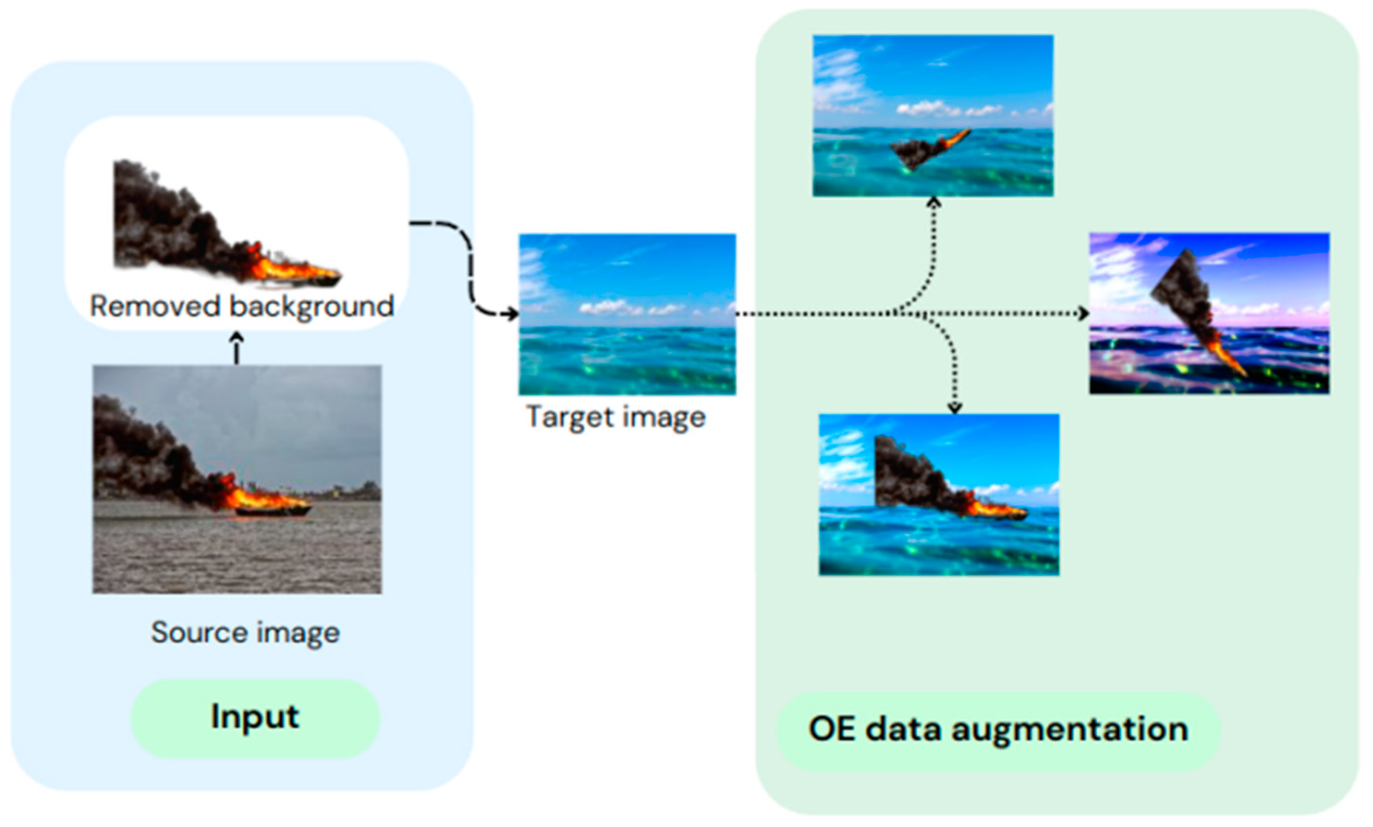
Several studies have proved the advantage of data augmentation in ML to train DL models. In this paper, we propose comprehensive data augmentation techniques based on image blending. By automatically removing the background from source images and integrating these into various target image backgrounds, we can create a vast and diverse dataset that simulates numerous real-world conditions.
Figure 1 is an example of a data augmentation illustration with basic and advanced data augmentation techniques combined, which is our proposed approach.
As previously mentioned, D-CNNs perform well in CV tasks with big data applications. This research focused on handling data scarcity related to ocean vessels. We augmented ship fire images by blending source and target images, where the source image is a ship on fire and the target images are various ocean environment scenes. To augment, backgrounds of ship fire images are removed and then attached to source images. During blending, we applied basic and advanced augmentation approaches. In
Section 3, we describe in more detail the methods that we utilized in this work. We anticipate that applying augmentation techniques, such as noise injection and scaling methods, for example, will significantly enhance the robustness of our generated dataset. These techniques enable us to create hazy ocean environmental images and simulate faraway distance localization, which in turn aid in improving the detection and recognition of small objects. To see the proposed method’s assistance in better image classification, especially ship fire detection, we fine-tuned Yolo (You Only Look Once) models, such as Yolo-v8 and Yolo-v10, and compared our achievements with other Yolo-based methods in
Section 5.
The main contributions of this research are as follows:
Collection of ship and ship fire images from internet sources.
Object-extracted blending of collected images with basic and advanced approaches. To note, our study will not cover all techniques of basic and advanced approaches.
Open-source Gradio web application for data augmentation that we applied in our work. Application can be used for the creation of other limited datasets.
To provide a comprehensive understanding of our research on data augmentation for the ship fire dataset, we have structured the sections of this paper accordingly as follows:
Section 2 is about related research works. This section provides a review of existing literature on data augmentation, focusing on various methods, datasets, and algorithms that have been studied.
Section 3 explains the contributions of this study. This part details the unique contributions of our research, specifically focusing on the techniques we employed for data augmentation in the context of ship fire images with blending to various ocean environment images. The key point is to include relevant data and techniques, such as background removal and blending with various ocean images by random location of the source image in the target image. Blending methods include random location, noise injection, rotation, cropping, scaling, and color and contrast change applications. In
Section 4, we highlight the development and functionality of the Gradio web application, created to facilitate the testing and visualization of our data augmentation techniques. The final section,
Section 5, summarizes the potential research directions and key contributions.
3. Proposed Methods, Model Architecture
3.1. Background Removing
From
Section 2, we have seen that by artificially enlarging the training dataset through various transformations, the application of data augmentation is becoming significantly helpful to develop a robust model by mitigating overfitting, covering scarce datasets, improving model generalization, and boosting overall accuracy. In this research, we propose a data augmentation approach that involves blending source and target images, applying a suite of augmentation techniques during the blending process. These techniques include random application of background-removed ship fire images while blending to source ocean images. Random application is crucial in every technique that we use in blending. These techniques include random resizing, cropping, blurring, positioning, color change, and usual flipping approaches.
Background removal, a specific form of augmentation, has gained prominence for its ability to isolate objects of interest from non-essential elements in an image. The image background removal library we use in our project was developed by Daniel Gatis. Removing the background from images is a technique used in image processing where the non-essential parts of an image are excluded, leaving only the foreground objects of interest. This process typically involves distinguishing the primary subject from the background using algorithms such as thresholding, edge detection, segmentation, and deep learning-based models. In our approach, the initial step was set to target image, where we focused on the primary subject and removed its background. For a given image I, represented as a matrix of pixel values:
where M and N are the dimensions of the image, and
denotes the pixel value at position (
).
Next, a segmentation algorithm is applied to divide the image into regions, producing a segmentation mask S:
where
is a binary value indicating whether pixel (
) belongs to the foreground (1) or the background (0).
After that, the processed image I’, after background removal is obtained by element-wise multiplication of the original image I and the segmentation mask S:
where, ∘ denotes the Hadamard product (element-wise multiplication).
The blending image function is designed to seamlessly overlay a ship image onto a background image at a specified position, ensuring proper handling of transparency. This function accepts three parameters, as can be seen in
Table 3.
The RGBA conversion ensures whether the background image supports transparency by including the alpha channel. The alpha channel acts as a mask in its represented channels to delineate the transparent and opaque regions of the ship image. The mask confirms that only the non-transparent parts of the ship image are pasted onto the background, allowing for smooth blending and preserving the visual integrity of both images.
3.2. Image Resizing and Positioning
The input image is converted to the RGBA mode to ensure the image has four channels, such as red, green, blue, and alpha—transparency. The inclusion of the alpha channel is particularly important for preserving transparency information, which is crucial when compositing the resized image onto different backgrounds. The dimensions of the resized image are computed by multiplying the original width and height of the ship image by the scale factor value. This step involves the use of integer typecasting to ensure the new dimensions are whole numbers. The image is resized to the newly calculated dimensions using the LANSZOS resampling algorithm, which is a popular method for image scaling.
To simulate different scales and perspectives, the isolated object is resized using a scaling factor. This is randomly selected within a predefined range to ensure variability. The resized object is then positioned onto the source image at random coordinates, creating a natural appearance of the object within different contexts.
Scaling by a factor of s:
where (
) are the coordinates in the original image, and (
) are the coordinates in the scaled image.
A more formal representation of the LANCZOS resampling process for a discrete set of pixels as follows in the equation below:
- -
is the original pixel value at position .
- -
is the resampled pixel value at the new position .
- -
is the Lanczos kernel applied to the distance between the original and new pixel positions.
3.3. Random Flip, Rotation and Combination
The input image was rotated at random angles to simulate different orientations. It was then combined with the target background image using blending techniques that ensure smooth integration and natural appearance. This step resulted in a final augmented image that was saved for further usage.
Vertical flip:
where I(
) is the pixel at coordinates (
) in the original image, W is the width, and H is the height.
Rotation by and angle
:
where (
) are the coordinates in the original image, and (
) are the coordinates in the rotated image.
3.4. Blur Effects
We applied the Gaussian blur effect to simulate various levels of atmospheric effects and depth of field. Noise injection is a matrix value usually drawn from a Gaussian distribution [
4], and it can help networks learn more robust features. Our work covers noise injection to prevent the model from learning the noise in the training data, which can lead to overfitting. By making the model robust to noise, it learns to better generalize unseen data and reach training stability. Our noise injection equation is as follows:
where,
is Gaussian noise with mean
and variance
.
In the next step, we applied a blur filter to the image. The Gaussian blur is a smoothing operation that reduces the high-frequency components in the image, effectively introducing an atmospheric effect. We set the blur radius from 1 to 20 and applied it to the blended ship image at random values. From the Gradio web app, the user can set blur ratio to zero, depending on their purpose [
64,
65].
3.5. Change Color Channels and White Balance Adjustment
Lighting biases are one of the most frequently facing challenges in image recognition tasks. Digital image data are typically represented as a tensor with dimensions corresponding to height, width, and color channels [
4]. Chatifled et al. [
43] mention that there is a 3% accuracy drop between grayscale and RGB image classification.
Implementing augmentations within the color channel space is an effective and straightforward form for individual color channels.
where
represent the red, green, and blue channels, respectively.
The white balance function is designed to correct color imbalances between target ship images and source ocean background images by performing white balance adjustment. With this, we ensure that colors in the image appear natural and accurate under varying lighting conditions. Proper white balance adjustment is crucial for maintaining color fidelity, especially in applications such as digital photography and image analysis or visual perception studies.
To calculate average intensities of each color channel, we have
:
where,
represents the intensity of the
i-th pixel in channel
c, and
N is the total number of pixels in the channel.
Afterwards, we compute scaling factor of channel
c as:
where avg is the average intensity computed across all channels.
Last, we adjust pixel intensities of
in channel
c using:
3.6. Change Contrast Button and Equalize Histogram
The contrast of the image is randomly adjusted to simulate different lighting conditions. This technique is used to improve the contrast of the image, making the objects more distinct.
where
is the contrast factor, and
is the mean intensity of the image.
The histogram equalization function is pivotal in preprocessing images for various computer vision tasks. Histogram equalization adjusts the cumulative distribution function (CDF) of pixel intensities to enhance contrast. By enhancing the contrast through HE, the function ensures that the images exhibit a more uniform distribution of pixel intensity. The process can be described mathematically as follows:
First, we compute the CDF
where
N is the total number of pixels in the image.
Next, we compute the map intensity values by transforming each pixel intensity
as:
where L is the number of possible intensity levels, and
is the new intensity value.
3.7. Change Sharpness Button
Then, we enhance image sharpness in a random range as we applied to other augmentation methods. The sharpness of the image is varied to simulate different camera focus settings.
where
is the sharpness factor, and
is the detailed enhanced image.
By iterating the above steps multiple times with different sources and target images, a massive dataset can be generated. Each iteration introduces random variations in scaling, positioning, rotation, blurring, color change, noise injection, and other OE-focused methods, resulting in a highly diverse and comprehensive dataset [
66,
67,
68].
3.8. Random Crop Function
We aimed to perform a random cropping (erasing) operation in an input image. This technique is a common data augmentation method used to increase the diversity of training datasets by generating multiple variations of the original image. Random cropping can help improve the robustness and generalization of ML models by providing a wider range. In this approach, we randomly cropped sections from background images after both target and source images were blended. This cropping might even crop ship fires images as well. The rectangular region is set to 500 by 500 in height and width, respectively. From the Gradio web app, it is possible to specify the height and width of a random rectangle area.
Image cropping (random erasing [
69]) is a common technique in image processing and data augmentation. In image recognition, this method mainly focuses on overcoming occlusion-related challenges, such as unclear part representation on objects. Mathematically,
is the image dimensions of width (
) and height (
) of the image. The goal is to crop a region of size (
,
) randomly from
, where
and
are the width and height of the cropping image region. For cropping coordinate detection, we randomly selected the top-left corner of the cropping region. Let
be the coordinates, then:
where,
is a function that returns a random integer between
and
.
We then set a transparency to that cropped area, denoted as
in transparent image size
,
. The transparent region
is then pasted onto the original image
with transparency. This result in
is given by:
This equation indicates that the region starting at (x,y) and extending pixels in width and pixels in height is replaced by the transparent region This process effectively creates an occlusion in the image, simulating scenarios where parts of the object are hidden. As we mentioned above, we have developed a Gradio web app, an interface to facilitate an interactive platform for performing and visualizing various image augmentation operations.
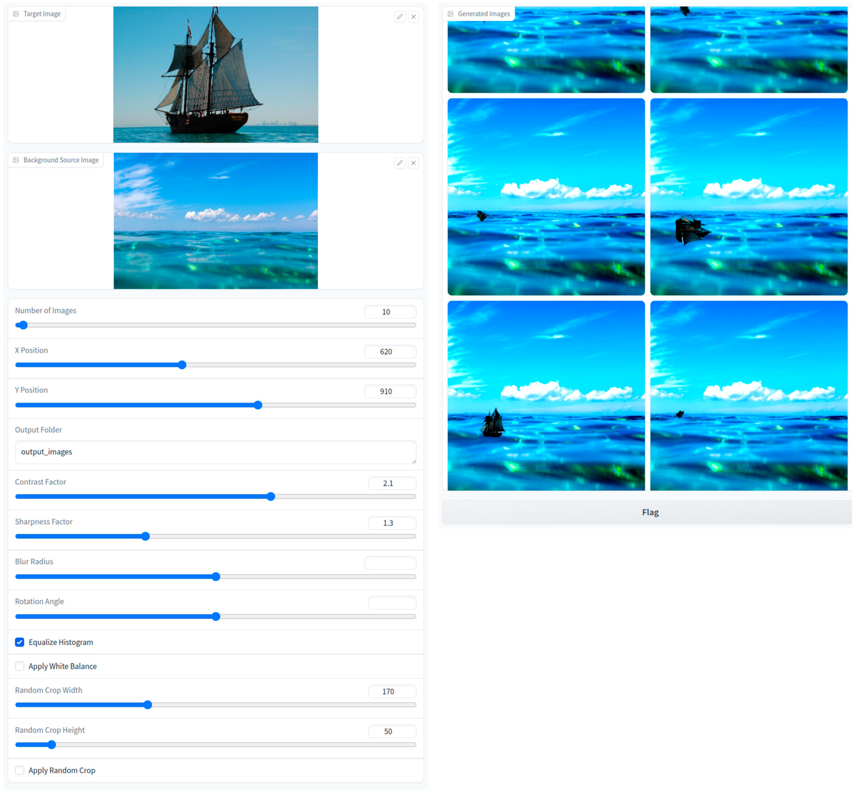
This system enables users to upload a target and a background image to generate a set of augmented images with varying parameters. In
Table 4, we can see the selection values of data augmentation. Based on the given features, data augmentation parameters can be customized. For example, if you want to have a bigger cropped area on the image by width or height, it is adjustable, ranging from 10 to 500. Similarly, other parameters are also available to select certain range values.
3.9. Dataset Collection
Figure 2 depicts the Gradio web interface, where we have an input target and source image. By sliding the OE augmentation method included functions, we can adjust data generation into our project.
Table 5 provides a detailed summary of the image dataset utilized for the task of ship fire detection, including both original internet source images and their augmented counterparts. The datasets are categorized into two primary classes, such as “Fire” and “No-fire”, with a further distinction between internet-sourced images and augmented samples in combination with ocean background images. For blending, the background should be a kind of image that represents all kinds of ocean scenarios. Similarly, sea vessels also should be varied, as the ocean environment covers many kinds of sea vessels. The initial dataset comprises 9200 images of ship fires and 4100 images of ships without fire. To increase the dataset size, a sample of 90 ship fire images was subjected to augmentation, resulting in an expanded dataset of 11,440 images. The extended dataset is generated by blending with 13 background ocean images.
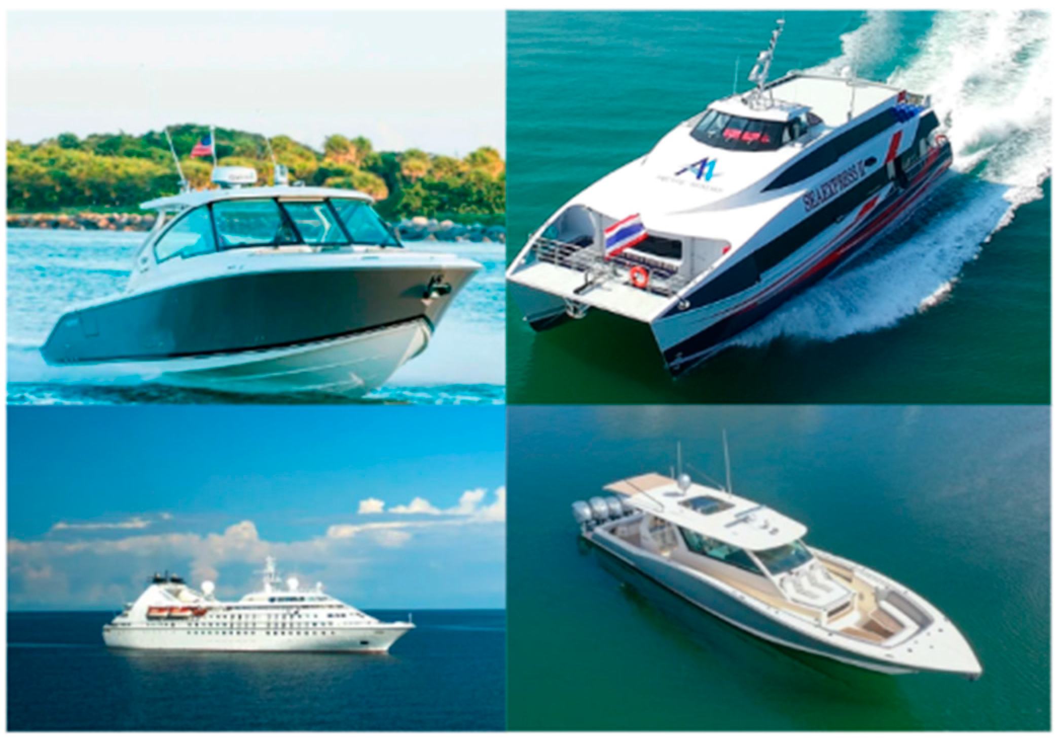
Figure 3 depicts a sample of ship images in an ocean environment. Ships in the image are considered as main objects that are extracted from the background and combined with other ocean images. Ocean and ship images are target and source images, respectively. Of these images, we augment one single-source ship image with another ocean target image. However, during blending source and target image, we can increase the number of images.
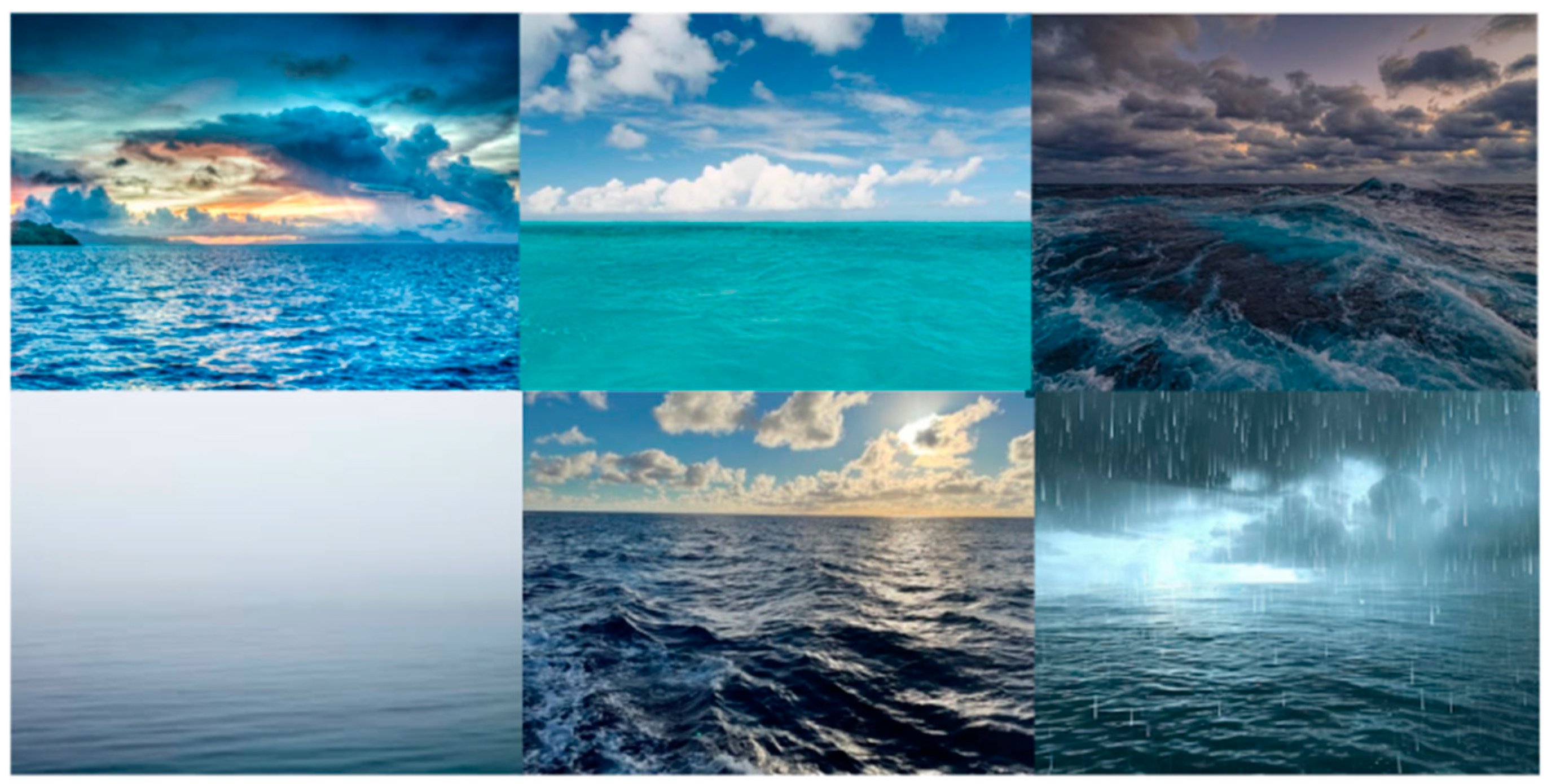
In
Figure 4, various different ocean environments are represented. An extracted ship image can represent various parts of an ocean image in applied augmentation techniques, such as noise injection (blur effect), rotation scaling, and random cropping techniques.
4. Experimental Results
In this research, we proposed several data augmentation techniques to source and target images for the purpose of ship fire image classification improvement. In
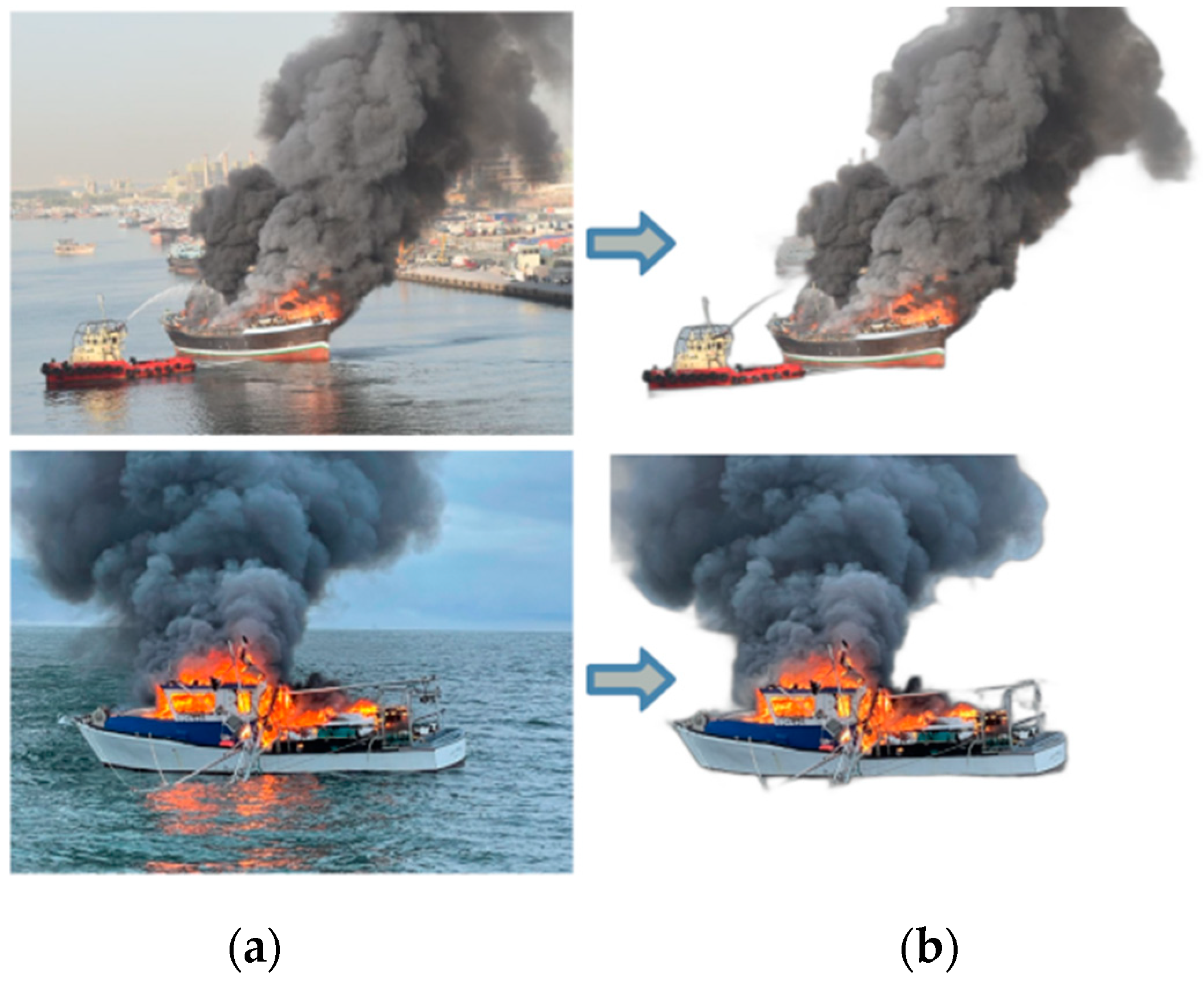
Figure 5a, a sample ship fire (boat) image is represented. From
Figure 5a, the main target image is extracted from the ocean environment and shown in
Figure 5b. This is the initial step for data augmentation.
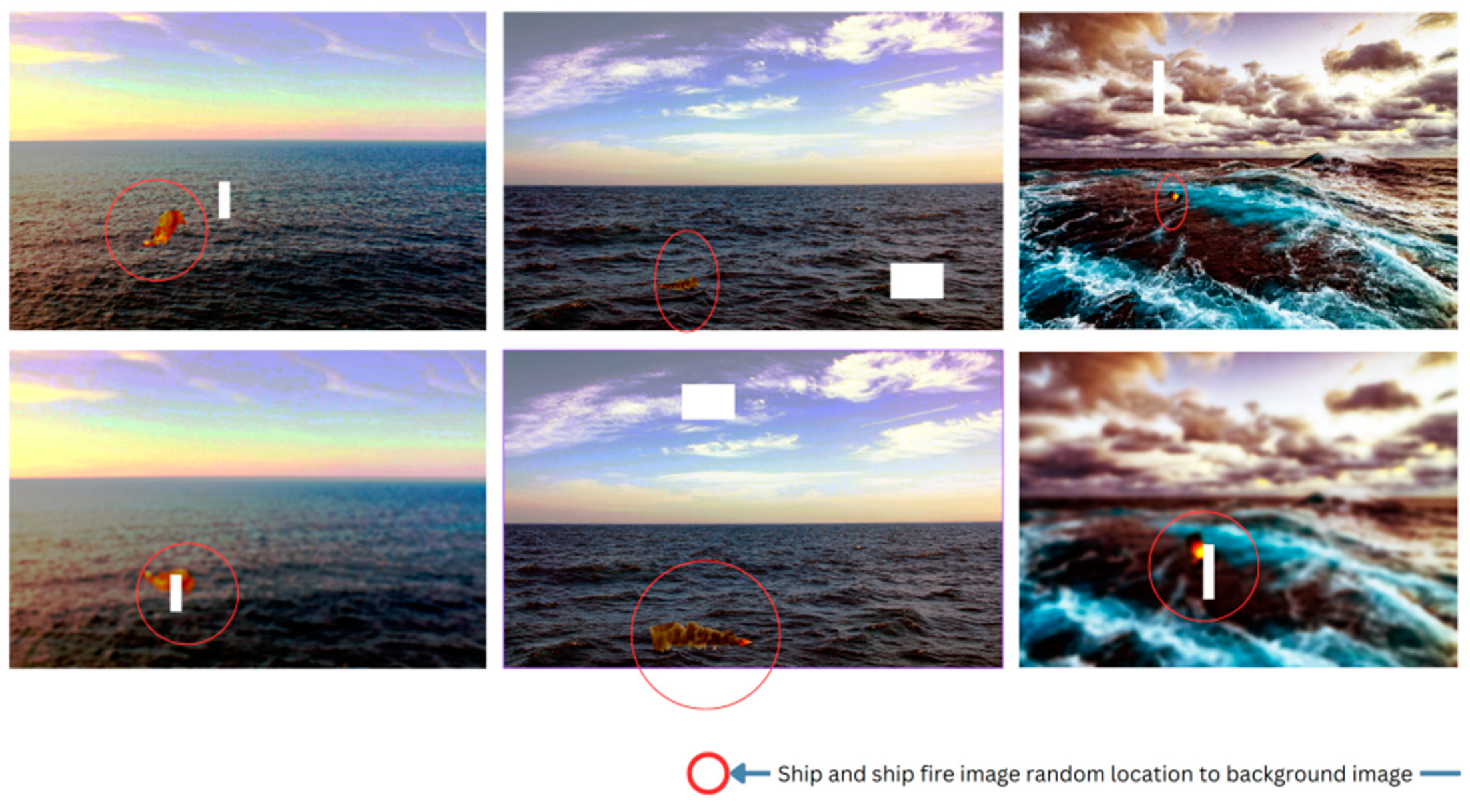
In
Figure 6, OE target images are attached to source ocean background images. In the red circles, we highlighted the source image location in the ocean image. As can be seen, augmentation techniques change the ocean image blur effect, sharpness, and a ship image’s random locations. Using the Gradio web application, we can change the source image location in the
x-
y axis and all other mentioned metrics listed in
Table 4. Finally, in
Figure 7, we see the OE ship fire dataset creation process beginning with the input ship fire image as the source and progressing to the extraction step, blending to target the ocean background image with the application of the data augmentation techniques.
To compare the augmented dataset performance, we labeled our dataset and trained the labeled dataset in Yolo-v8 and Yolo-v10 versions. Both models’ classification accuracy was high; therefore, we chose these models to fine-tune for ship fire detection purposes.
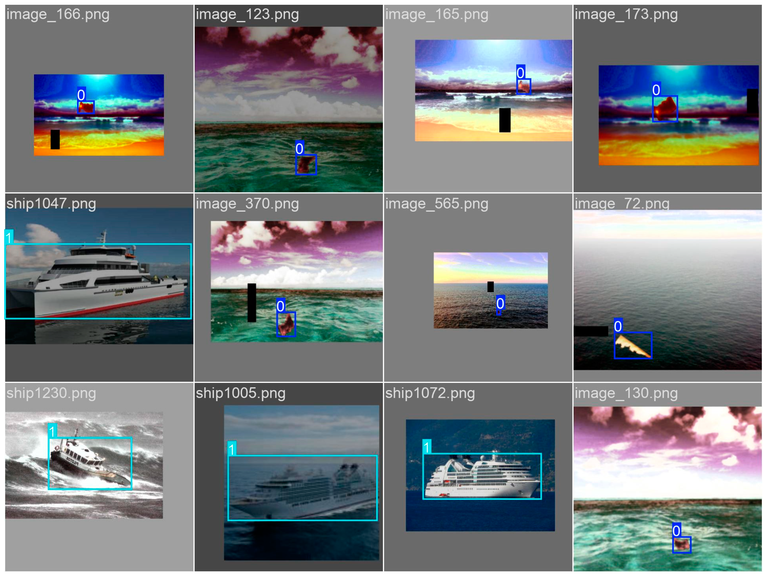
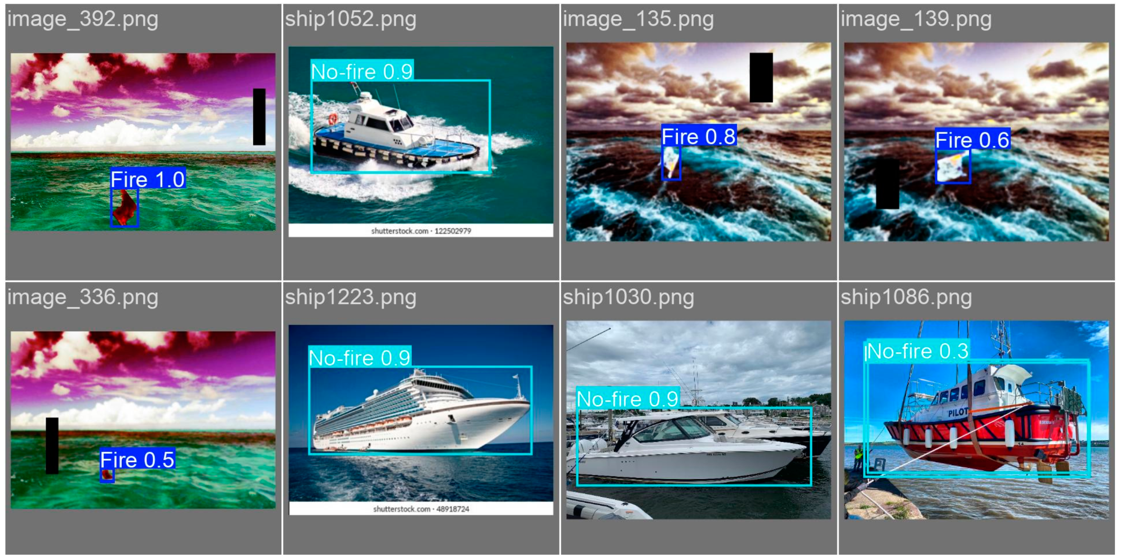
Figure 8 and
Figure 9 show training image examples with bounding box information on labeled classes. From figures, we can see that ship images are relatively clear to distinguish and identify, which is the “No-fire” class dataset. However, in the “Fire” class, we achieved our proposed style of dataset and type. In other words, we obtained hazy ship fire images with a different look, scale, size, and other applied augmentation technique results. From the comparative analysis of
Table 1, it can be concluded that having a large variety of datasets increases the model’s detection and classification accuracy.
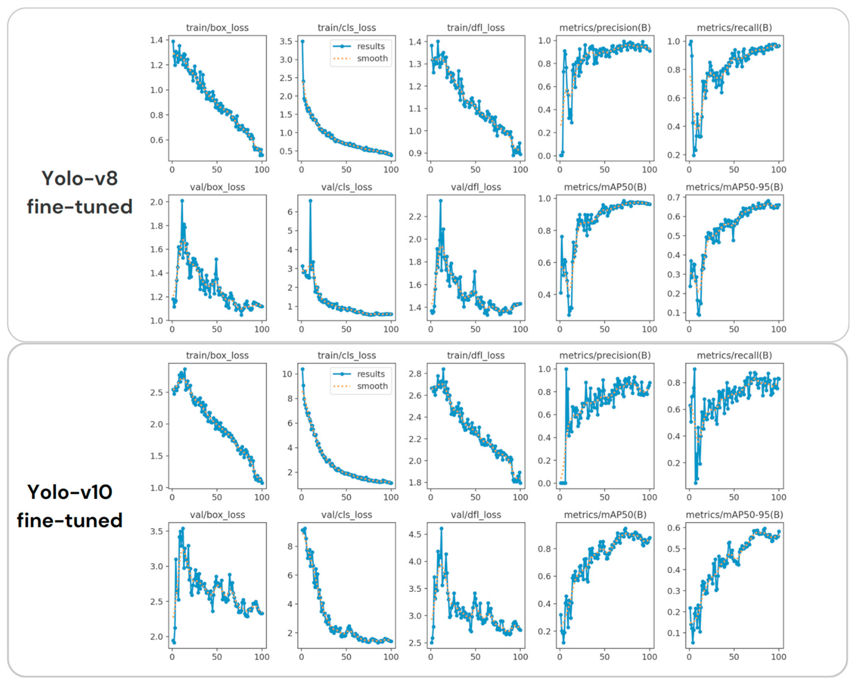
We trained both models on 100 epochs (
Figure 10). The training and validation loss plots show a decreasing trend, indicating that the models are improving as training progresses. The loss curves appear smoother, but there are some fluctuations in both models’ cases, possibly due to challenges in model optimization. In comparison, training and validation losses for the Yolo-v10 fine-tuned model for ship fire detection are consistently lower and smoother compared to Yolo-v8.
Metrics, such as precision, recall, and mean average precision (mAP), improve over epochs but show irregular behavior, especially after 50 epochs. These fluctuations are considered as our future research work that we focus on to optimize model training and solve instability in training or validation performances. The mAP score is a key metric for object detection tasks, measuring the accuracy of the bounding boxes. Yolo-v10 showed a higher and more consistent mAP than Yolo-v8, which demonstrates that the fine-tuned Yolo-v10′s performance is higher at detecting and classifying ship fires.
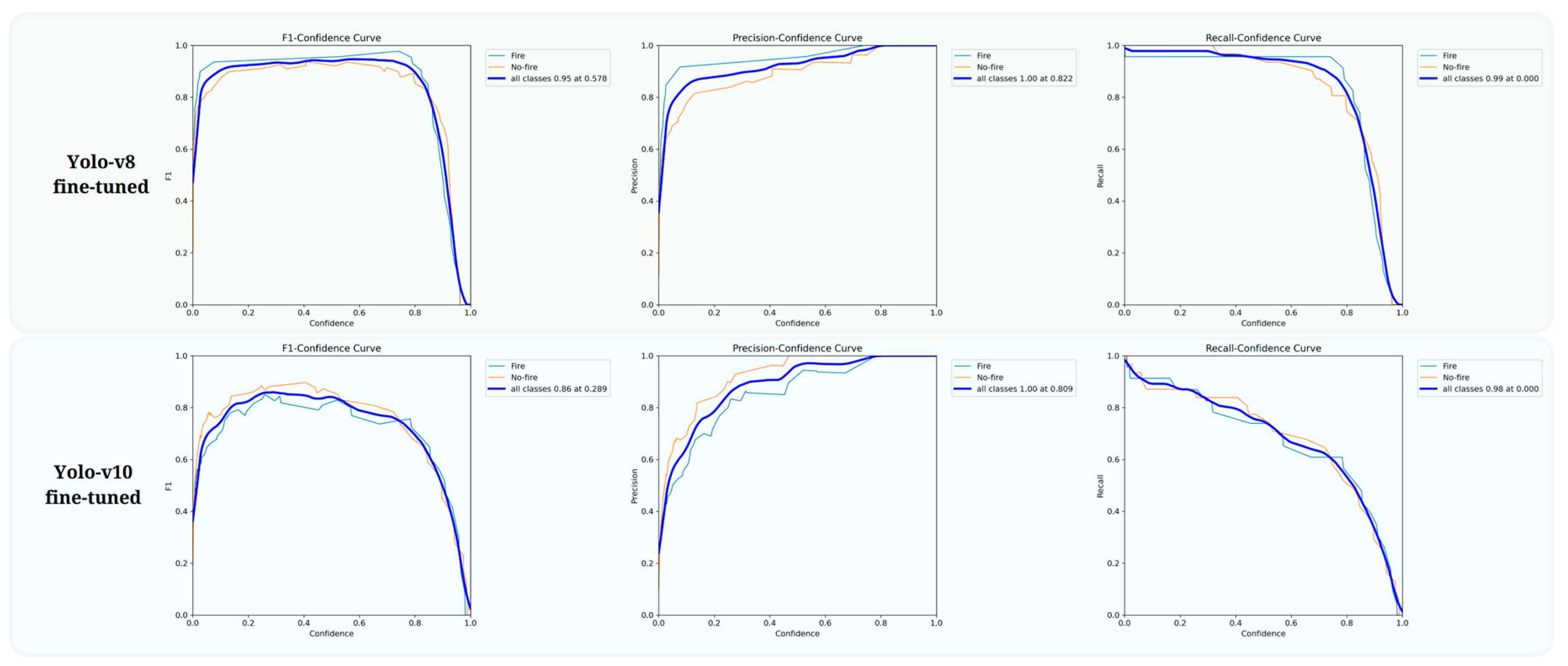
In
Figure 11, precision-recall (PR) curves are presented to illustrate the performance of both models’ training. In Yolo-v8, the mAP at the intersection over union (IoU) threshold of 0.5 reached 0.91% accuracy, which demonstrates the model’s relatively high accuracy in detecting and classifying ship fires. The PR curve for Yolo-v10 demonstrates slightly improved precision at 0.913 and recall of 0.937, indicating a better balance between precision and recall compared to Yolo-v8. However, in terms of Yolo-v8, the exact scores were 0.866 and 0.912 in precision and recall metrics. The mAP score of Yolo-v10 at the IoU (
[email protected]) is also higher for Yolo-v10 at 0.937, as can be seen in
Figure 11 and
Figure 12.
Table 6 compares the ship fire detection models’ achievements. Applied data augmentation and blending techniques for ship fire image, the custom fine-tuned models, such as Yolo-v8 and Yolo-10, clearly outperformed the more generalized models like, Yolo-v3-Tiny, Yolo-v5s, and Yolo-v7-Tiny. The fine-tuned Yolo-v10 model stands out, delivering the best precision, recall, F1 score, and
[email protected], which indicates proposed method superiority for accurately detecting ship fires in diverse ocean environments.
6. Conclusions
In this study, we presented an OE data augmentation technique based on image blending, which involves automatically removing backgrounds from source images and combining them with target images. This method allows for the generation of massive and diverse datasets, enhancing the training and generalization capabilities of ML models. Nowadays, many researchers focus on GAN, or style transfer architectures, as a focus area of interest. However, GANs can produce synthetic data with artifacts and noise that do not appear in real data and require significant computational resources. Perez et al. [
73], for example, proposed a neural style transfer algorithm that required two images from samples. However, the style transfer augmentation approach did not have any impact on the MNIST problem, which is the generation of a numerical dataset. Our approach is superficial with keeping OE identity by avoiding unrealistic subtlety, which cannot mislead the training process and degrade model performance. Moreover, our proposed OE data augmentation methods can iteratively generate huge amount of data, so that training of ML models does not suffer from a lack of data and diversity.
We used a dataset of ship images and an ocean image as a background to blend ship images in ocean environments. The ship images were processed using the background removing algorithm. The resulting isolated ship images were then merged with the source background image and blended into the OE augmentation pipeline.
In our future work, we will focus on optimizing data augmentation functionalities even further and wish to combine with Yolo (You Only Look Once) models to automate CV model training processes in a more straightforward manner.


