Abstract
High-speed microjet hydrogen–air diffusion flames are investigated computationally. The focus is on the prediction of the so-called bottleneck phenomenon. The latter has been previously observed as a specific feature of the present flame class and has not yet been investigated computationally. In the configuration under consideration, the nozzle diameter is 0.5 mm and six cases with mean nozzle injection velocities (U) between 306 m/s and 561 m/s are considered. The flow in the nozzle lance is analyzed separately to obtain detailed inlet boundary conditions for the flame calculations. It is confirmed by calculation that the phenomenon is mainly determined by the transition to turbulence in the initial parts of the free jet. The transitional turbulence proves to be the biggest challenge in predicting this class of flames, as the generally available turbulence and turbulent combustion models reach the limits of their validity in transitional flows. In a Reynolds-Averaged Numerical Simulation framework, the Shear Stress Transport model is found to perform better than alternative two-equation models and is used as the turbulence model. By neglecting the interactions between the turbulence and chemistry (no-model approach), it is possible to predict the morphology of the bottleneck flame and its dependence on U qualitatively. However, the position of the bottleneck is overpredicted for U < 561 m/s. The experimental flames in the considered U range are all attached to the nozzle. This is also predicted by the no-model approach. The Eddy Dissipation Concept (EDC) used as the turbulence combustion model predicts, however, lifted flames (with increasing lift-off height as U decreases). With the EDC, no bottleneck morphology is observed for U = 561 m/s. For lower U, the EDC results for the bottleneck position are generally closer to the measurements. It is demonstrated that accuracy in predicting the bottleneck position can be improved by ad hoc modifications of the turbulent viscosity.
1. Introduction
Parallel to the increasing utilization of renewable energy sources, together with sustainable energy management and recovery technologies [1,2,3], energy conversion through combustion will continue to play an important role, with an increasing emphasis on clean combustion. In the case of solid fuels and waste, in addition to combustion [4,5], gasification [6] is a good option for clean power generation. The synthesis gas contains considerable quantities of the “clean fuel”, hydrogen. In their recent experimental work, Sarker et al. [7] reported a hydrogen selectivity of up to 52% in the gasification of agricultural residues. Furthermore, the production of hydrogen by nuclear power plants is attracting increasing interest as a potential solution for the elimination of fossil fuels in the context of green energy supply [8,9]. In addition, hydrogen represents a very interesting alternative for the storage of surplus power from renewable power generation from wind turbines and photovoltaic systems [10].
In this context, combustion based on hydrogen and hydrogen mixtures has great potential to enable a clean and sustainable energy supply in the future. In areas such as stationary gas turbines, premixed combustion has been the state of the art. This has proven to be an extremely effective means of reducing the formation of thermal NO. One of the main problems with the premix combustion is so-called “flashback” [11]. Compared to methane, or other hydrocarbon fuels, hydrogen is much more reactive and has a much higher burning velocity. Although current technologies based on conventional fuels have been able to cope with the flashback problem, the use of hydrogen or hydrogen mixtures in premix systems poses a major challenge due to the higher flashback propensity. In a recent study, Aniello et al. [12] investigated the hydrogen substitution of natural gas in premixed perforated burners experimentally and confirmed the increase in the tendency to flashback due to the addition of hydrogen. Therefore, the investigation of flashback mechanisms and methods for preventing flashback in the context of hydrogen fuel utilization is increasingly moving into the focus of researchers.
Kudriakov et al. [13] numerically investigated a premixed laminar hydrogen flame in the presence of a quenching mesh. They were able to predict quenching qualitatively, but without a quantitative assessment. In a swirling hydrogen flame, Schönborn et al. [14] discovered experimentally that the flame eccentricity (caused by the precessing vortex core) can have an inhibiting effect on flashback. In a more recent study, Kiymaz et al. [15] carried out a numerical investigation of laminar premixed methane–hydrogen flames with a focus on the flashback dynamics, emphasizing the role of the wall temperature for the flashback tendency.
In order to prevent flashback, a completely different approach is to resort to non-premixed combustion, in which flashback is categorically impossible [11]. Recently, researchers are increasingly turning their attention to non-premixed technology to reduce flashback. Lopez-Ruiz et al. [16] analyzed a domestic multi-flame diffusion burner for hydrogen operation. Li et al. [17] investigated the effect of the addition of hydrogen on the structure of the microjet methane diffusion flame. Turbulent hydrogen diffusion flames were analyzed by Haj Ayed et al. [18] in connection with combustion in gas turbines.
On the other hand, if combustion takes place in the diffusion mode, local temperature peaks are unavoidable. For providing high local formation rates of thermal nitrogen oxide (NO) in this case, countermeasures exist such as dilution of the flame zone by exhaust gas recirculation or shortening the residence time. For realizing the latter, the use of microjet flames [19] has recently emerged as a convenient means. Against this background, the present work addresses microjet hydrogen diffusion flames, which are increasingly receiving attention, not only as a means for reducing NO emissions, but also for their relevance to compact applications.
In their rather recent experimental work on microjet hydrogen flames, Kozlov et al. [20,21,22] and Shmakov et al. [23] drew attention to a particular flame pattern, which constitutes the particular focus of the present investigation. The observed flame pattern was termed as the “bottleneck flame” [20,21,22,23]. Here, the radial expansion of the flame is quite large near the nozzle, narrows down abruptly at a certain distance from the nozzle and then expands again, resulting in the so-called bottleneck shape. This flame pattern was previously observed experimentally by other researchers [24,25], but not elaborated further. Kozlov et al. [20,21,22] and Shmakov et al. [23] have brought it back into the focus of current interest with their more recent studies. The purpose of the present paper is to present a computational study of this phenomenon, investigate its predictability by the available computational methods and, in doing so, to evaluate the predictive capability of the latter. To the best of the authors’ knowledge, this phenomenon has not yet been investigated computationally, which makes up the novelty of the present work.
Flames of gaseous fuels have received much attention from researchers in the past [26,27]. Although the flames of hydrocarbon fuels have been more in focus, there is still a large body of work on hydrogen flames. The numerous earlier papers on premixed hydrogen flames deal with topics such as flame propagation and safety [28,29,30,31]. An experimental and numerical study on laminar, nitrogen-diluted hydrogen diffusion flames was presented by Toro et al. [32]. A further numerical study on the same flame was presented by Piemsinlapakunchon and Paul [33], addressing the NO emissions. Skottene and Rian [34] studied the NO formation mechanisms in counterflow laminar hydrogen flames, based on a one-dimensional formulation. Benim and Korucu [35] presented a computational analysis of the flame of Toro et al. [32] with a more detailed analysis of various modeling aspects and NO formation paths. Benim et al. [36] and Benim and Pfeiffelmann [37] presented computational studies of lifted turbulent diffusion hydrogen flames, comparing the predictive capability of different turbulent combustion models. Haj Ayed et al. [18] presented a study on microjet diffusion flames for reducing NO emissions during combustion in gas turbines. A continuation of the work was published by Funke et al. [38], where more sophisticated models for turbulent combustion were applied. In none of the previous computational studies on laminar or turbulent hydrogen diffusion flames was the “bottleneck flame” phenomenon observed or addressed.
In the present work, the predictive capabilities of different modeling approaches for the present class of flames, i.e., for high-speed microjet hydrogen–air diffusion flames exhibiting a bottleneck structure, are investigated and assessed. The current computational analysis is based on the finite volume method based on general-purpose CFD code ANSYS Fluent 2022/R2 [39].
2. The Test Case
The high-speed microjet hydrogen–air diffusion flames measured by Kozlov et al. [20] are computationally analyzed. A sketch of the experimental device [20] is provided in Figure 1.

Figure 1.
Sketch of experimental device of Kozlov et al. [20].
Leaving the plenum, the pure hydrogen flows upwards through a vertically oriented circular tube (nozzle) with the length (L) of 60 mm. Beyond the nozzle exit, it forms a free jet, while mixing with the ambient air, and burns in the diffusion combustion mode (Figure 1). Two microjet nozzle diameters (d) were considered in the experiments, i.e., 0.5 mm and 1.0 mm [20]. In the present work, the flames with d = 0.5 mm are considered only (Figure 1). As far as the geometrical details are considered, the information provided in Ref. [20] was not complete. Therefore, when needed, assumptions had to be made. It is assumed that the flame is not confined and an atmospheric free jet flame results.
The operation conditions for the flames were provided only in terms of the area-averaged nozzle velocities (U) [20]. In total, 10 flames with different nozzle velocities were measured. The experimentally obtained [20] shadowgraph images of the flames for the six considered cases are provided in Figure 2.
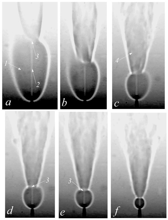
Figure 2.
Experimental shadowgraph images of high-speed microjet hydrogen–air diffusion flames for different mean nozzle velocities U (m/s): (a) 306, (b) 357, (c) 408, (d) 459, (e) 510, (f) 561 (Kozlov et al. [20]. The numbers in the sub-figures stem from the source [20], but they are not referred to in the present discussions).
The so-called bottleneck shape of the flame can easily be observed in Figure 2. It is most pronounced for the lowest nozzle velocity, i.e., for U = 306 m/s (Figure 2). A rather broad flame is formed just downstream from the nozzle. This becomes narrowed down further downstream, forming the “bottleneck”, and expands thereafter. This behavior is attributed to transition to turbulence [20]. The bubble (bottle) size becomes reduced with the increasing nozzle velocity (Figure 2). At very high nozzle velocities, additional features were observed [20]. For U ≥ 612 m/s, lifted flames were reported. In the present work, the six flames in the lower velocity range are considered, namely the flames with nozzle velocities of 306 m/s, 357 m/s, 408 m/s, 459 m/s, 510 m/s and 561 m/s, which are shown in Figure 2. Due to the compressible nature of the flow, the velocity varies along the fuel lance by expansion. This creates some uncertainty with respect to the nozzle velocities given in Ref. [20], since their position of occurrence is not clearly stated [20]. It is currently assumed that the given velocities are those occurring at the nozzle outlet.
Based on the available information [20], a priori estimations on the flow state in the nozzle can be made. Assuming atmospheric static pressure and a static temperature of 288 K at the nozzle exit and ideal gas behavior, local dimensionless numbers at the nozzle exit such as the Reynolds number (Re) [40], Mach number (Ma) [40] and the Froude number (Fr) [41] can be calculated, which are listed in Table 1.

Table 1.
Flames with mean nozzle exit speeds and estimated dimensionless numbers at nozzle exit.
The present, expanding nozzle flow, with variable material properties, is obviously more complex compared to an incompressible, constant-property pipe flow. For the latter, the laminar flow regime is known to prevail for Re < ~2000, while a fully developed turbulence is assumed to occur for Re > ~3000–4000. Thus, transitional turbulence can be expected to play an important role for the current setup. Since the flow is expanding, a “fully developed” flow state, where the velocity undergoes no more change along the tube length, cannot be achieved (as long as the expansion continues). Still, available expressions for the developing length, for incompressible pipe flow, can be used for estimation purposes. They imply, for all cases, that the nozzle is not necessarily sufficiently long to assure fully developed conditions at the exit.
The Mach numbers (Table 1) indicate that one should account for the compressibility effects. It should also be noted that the Mach numbers appearing in the table are based on the area-averaged velocities. Considering the radial velocity distribution in the nozzle, one can realize that higher values are likely to occur locally, near the nozzle centerline.
3. Modeling Outline
3.1. Mathematical Modeling Overview
Differential balance equations for mass, momentum and energy, as well as the species mass fractions for the compressible flow of a reacting ideal gas mixture, are computationally solved [39,42,43,44,45]. Thermal radiation is considered via the P1 model [39,46]. The gas absorption coefficient is estimated through the available Weighted Sum of Gray Gases Model [47] framework of the used software (although the standard coefficients of the model were adjusted for CO2/H2O mixtures [39,48]). The mean path length is estimated by a “domain based” approach. Buoyancy is considered, although the Froude numbers (Table 1) indicate a momentum-dominated flow [41]. Viscous dissipation is taken into account, which is expected to play a role for the high-speed flow in the narrow nozzle. The isobaric heat capacities of the species are represented by empirical fourth-order polynomials of temperature. The molecular transport properties of the mixture are obtained through ideal gas mixing laws, where the transport properties of its components are based on kinetic theory. For the mass diffusion, full multi-component diffusion due to the concentration gradients (concentration diffusion), as well as thermal diffusion due to the temperature gradients (thermal diffusion), are considered.
For investigating the effect of the individual model ingredients, calculations are also performed neglecting the buoyancy, thermal diffusion and simplifying the mass diffusion. In such calculations, only one ingredient is changed at a time, while the others remain as described above.
3.2. Turbulence Modeling
From the above discussion, it is obvious that transitional turbulence [49] plays an important role here. Within an RANS (Reynolds-Averaged Numerical Simulation) framework [50,51], there are only a few turbulence models that explicitly claim to be able to predict transitional turbulence. One of the more sophisticated ones in this category is the four-equation Transition SST model (T-SST) [39,52,53,54]. However, like other models in this category, the model is designed to predict transition in the wall boundary layers of external aerodynamic problems, but not necessarily in free shear layers as in the present case. Nevertheless, it is considered as an option in the present study as no better alternatives are known. In our previous studies [55], we observed that the two-equation SST k-ω [39,56] model (SST) has some ability to predict transition. Thus, in the present work, the SST is also considered as the turbulence model. For comparison, the standard k-ε model (KE) [39,57] is also used, complementing it with the two-layer zonal method [39,58] for the near-wall flow.
The turbulence models are used with their standard (default) values of model constants, applying production limiters, including the model amendments to account for compressibility and buoyancy effects [39]. In all models and cases, the maximum values of the non-dimensional wall distance of the next-to-wall cells, y+ [39,50], are always kept below unity.
Given the potential inaccuracies in the prediction of transitional turbulence associated with RANS-based turbulence models, a time-dependent, turbulence-resolving method such as Large Eddy Simulation may be considered more appropriate [59]. However, it is obvious that such methods require very high computational resources compared to RANS-based methods. Therefore, in the current phase, the RANS-based methods are considered in order to explore their predictive capability first. In presenting the results in the following sections, the averaged nature of the variables will not be indicated explicitly. All quantities are to be understood as Favre-averaged [27].
3.3. Reaction Mechanisms
For modeling hydrogen combustion reactions, the global reaction mechanism of Marinov et al. [60] (consisting of a single irreversible reaction involving the main species H2, O2 and H2O) and the detailed reaction mechanism of Conaire et al. [61] (consisting of over 20 elementary reactions of 8 species, namely, H2, O2, H2O, O, H, OH, HO2, H2O2) are used.
3.4. Turbulent Combustion Modeling
Modeling the turbulence–chemistry interaction, i.e., turbulent combustion modeling, is a further challenge due to the transitional nature of the present flow. The commonly available combustion models essentially assume a fully developed, high Reynolds number turbulence. In the present work, a “no-model” approach is found convenient and adopted, where the turbulence chemistry interaction is neglected. For comparison, the Eddy Dissipation Concept (EDC) [39,62] is also employed as the turbulent combustion model.
3.5. Numerical Modeling
Differential governing equations are spatially discretized by the finite volume method [63]. Discretized continuity and momentum equations are solved by a coupled solver. For achieving a steady-state solution, a pseudo-transient formulation, with automatic time stepping, is applied [39,63]. The convective terms are discretized by a second-order upwind scheme [39,63]. Only in one case did a first-order upwind scheme [39,63] have to be applied for the turbulence quantities to achieve convergence. For the sake of comparability, this is, then, applied to all cases for turbulence quantities, without, however, a noticeable effect on the results. For the chemical kinetics, a stiff chemistry solver is employed [39].
4. Solution Domains
Since the geometry and boundary conditions exhibit a circumferential symmetry, the steady-state, or time-averaged solution, is to be symmetric. Therefore, a two-dimensional axisymmetric formulation can be applied, if a steady state (or time-averaged in the sense of RANS) is targeted.
Due to the uncertainties in the flow details at the nozzle exit, not only the flame, but the flow in the nozzle lance is also analyzed. Due to different natures of the flows, it is found convenient to analyze the flow in the nozzle and the flame not in a single, but in separate domains. The flow in the nozzle domain is analyzed, and the resulting nozzle outlet distributions are used as the inlet boundary conditions in the subsequent calculation in the flame domain. In a horizontal layout, the domains are sketched in Figure 3.
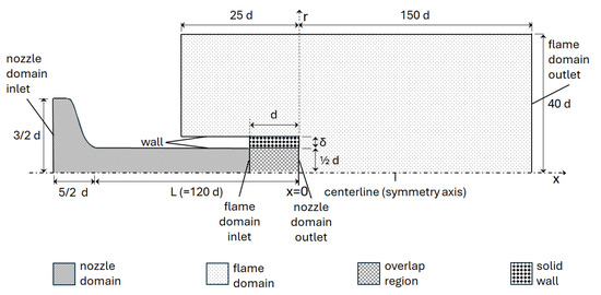
Figure 3.
Sketch of solution domains and boundaries for 2D axisymmetric formulation (not to scale).
Given the free jet configuration, the boundaries of the flame domain that separate the domain from the environment are not uniquely defined and to be chosen as a part of the modeling. They shall be positioned at a sufficient distance so as not to interfere with the flame. A domain size of 40 d in the radial direction and 150 d in the axial direction, measured from the nozzle outlet (Figure 3), is found to sufficiently fulfill this requirement. One can also see that the flame domain extends 25 d upstream from the nozzle outlet, for preventing any disturbing effect by the corresponding boundary.
5. Boundary Conditions
In Figure 3, one can see that the inlet of the flame domain is not placed exactly at the nozzle outlet, but a nozzle diameter (d) distance upstream in the nozzle. Thus, after the nozzle flow solution, not the results at the nozzle domain outlet, but those at the section one nozzle diameter upstream are used as the inlet boundary conditions for the flame domain. The tube wall section corresponding to this overlapping region is also included as “solid” in the flame domain, to be able to predict an eventual conjugate heat transmission form hot flame touching the tube, to the flow in the nozzle across the wall (Figure 3).
For the nozzle domain calculations, which are carried out for pure hydrogen as fluid, a constant, atmospheric static pressure is applied as the boundary condition at the nozzle outlet (assuming the static pressure variation in the flame domain to be negligible compared to that along the nozzle), assigning zero-gradient boundary conditions for the remaining variables. Obviously, the no-slip boundary conditions and the symmetry conditions apply at the wall and on the symmetry axis, respectively. For the energy equation, the nozzle walls are assumed to be adiabatic. At the nozzle inlet boundary, a constant total temperature and mass flow rate are applied as the boundary conditions. The total temperature is assumed to be 298 K, and the mass flow rate is iteratively varied until the target area-averaged velocity at the nozzle exit is achieved (Table 1).
Modeling turbulence in the nozzle is challenging due to transitional effects. Although the Reynolds numbers for the nozzle velocities (Table 1) imply a rather laminar flow state for some cases, for a unified and smooth treatment, a turbulence model is used for all cases, assuming that the model can predict transitional effects to an extent. As the inlet boundary conditions for the turbulence quantities, a very low turbulence intensity of 0.1% and a macro-length scale of 30% of the inlet diameter are assumed.
For the flame domain calculations, carried out for the mixture of ideal gases, the inlet boundary conditions for all flow variables, except pressure, are extracted from the preceding nozzle domain solution, as mentioned above. The mass flow rate along with the radial mass flux distribution are prescribed as the inlet boundary conditions for the momentum equations. Radial distributions of the total temperature and turbulence quantities are prescribed as well. Radial variations in the variables are described by polynomials up to fourth order, which very closely represent the obtained solution in the nozzle domain. The inlet boundary conditions for the species transport equations are trivial, since the flame domain inlet boundary lies within the nozzle. As the wall boundary condition for the energy equation, an adiabatic wall is assumed except for the walls corresponding to the overlapping region (Figure 3), where the fluid–solid coupled heat transfer is calculated. The tiny left boundary of the solid region (Figure 3) is assumed to be adiabatic.
At the outlet of the flame domain (Figure 3), a pressure boundary with constant ambient static pressure is applied. The further free boundaries that are placed radially at 40 d from the centerline and at −25 d from the nozzle exit (Figure 3) are also treated as pressure boundaries with a prescribed ambient static pressure. At the pressure boundaries, the flow direction is not prescribed. In case of outflow, zero-gradient boundary conditions apply and in case of inflow, assumed ambient values for temperature (288 K), species mass fractions (air composition) and turbulent quantities are applied. For the latter, again, a quite low turbulence intensity of 1% and a macro-length scale equal to 30% of the corresponding hydraulic diameter are assumed.
6. Grids
All grids are generated based on quadrilateral cells, arranged in a structured manner (except in a small region in the plenum of the nozzle domain). Grid independence is always assured.
Figure 4 shows the results of a grid independence study for the nozzle domain, for the highest nozzle velocity, using grids with 1400, 4400, 5400, 12,200, 21,600, 33,400, 48,600, 58,200 and 86,400 total number of cells.
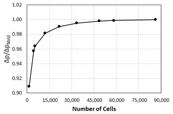
Figure 4.
Normalized pressure drop across nozzle calculated by different grids.
The pressure drop (Δp) across the nozzle is displayed (Figure 4), where the values are normalized by the maximum value, ΔpMAX, obtained with the finest grid. One can observe that the deviations are less than 1% for grids with a number of cells greater than 21,600. The finest grid with 86,400 is used for the calculations.
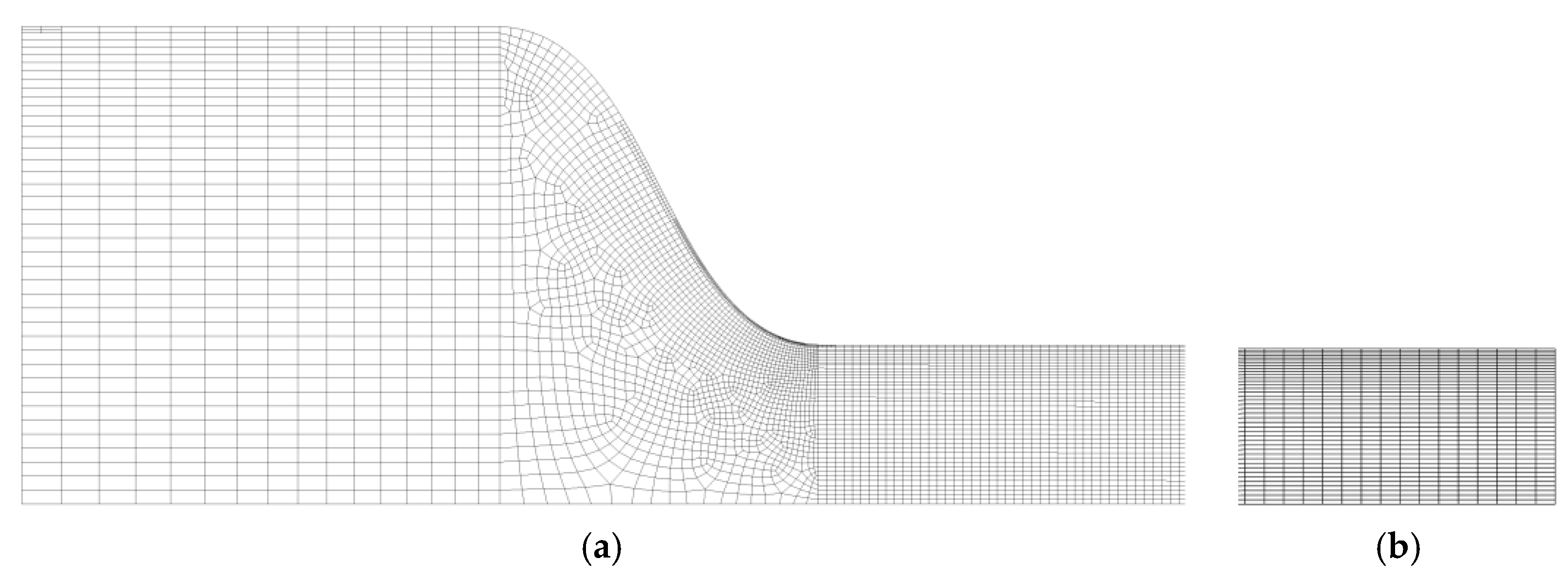
Detail views of the grid for the inlet and outlet regions of the nozzle domain are shown in Figure 5.
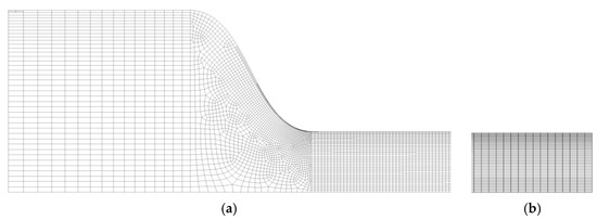
Figure 5.
Grid for nozzle domain: (a) detail view at inlet, (b) detail view at outlet.
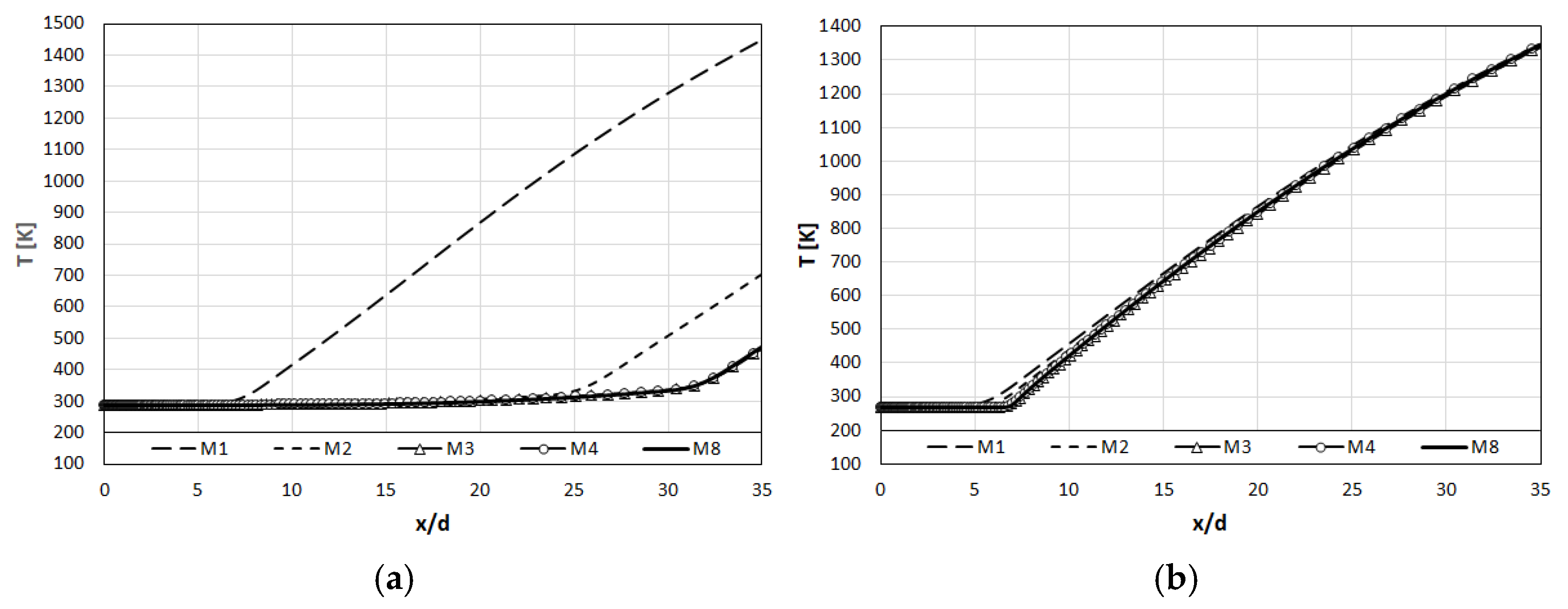
In the grid independence study for the flame domain, in total, eight grids with 9200 (M1), 16,800 (M2), 25,600 (M3), 33,400 (M4), 40,000 (M5), 45,200 (M6), 50,500 (M7) and 57,000 (M8) are considered. Temperature variations along the symmetry axis for Case A and Case F (Table 1) calculated by different grids are shown in Figure 6 for the nozzle nearfield, where the results obtained for M5, M6 and M7 are not shown for clarity. One can see that even with grid M3 (25,600 cells), a sufficient grid independence is achieved for both flames. Still, the finest grid M8 (57,000 cells) is used for the calculations, where a sufficient grid independence for all considered flames can be assumed.
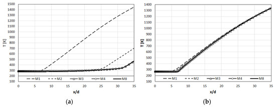
Figure 6.
Temperature variation along centerline calculated by different grids: (a) Case A, (b) Case B.
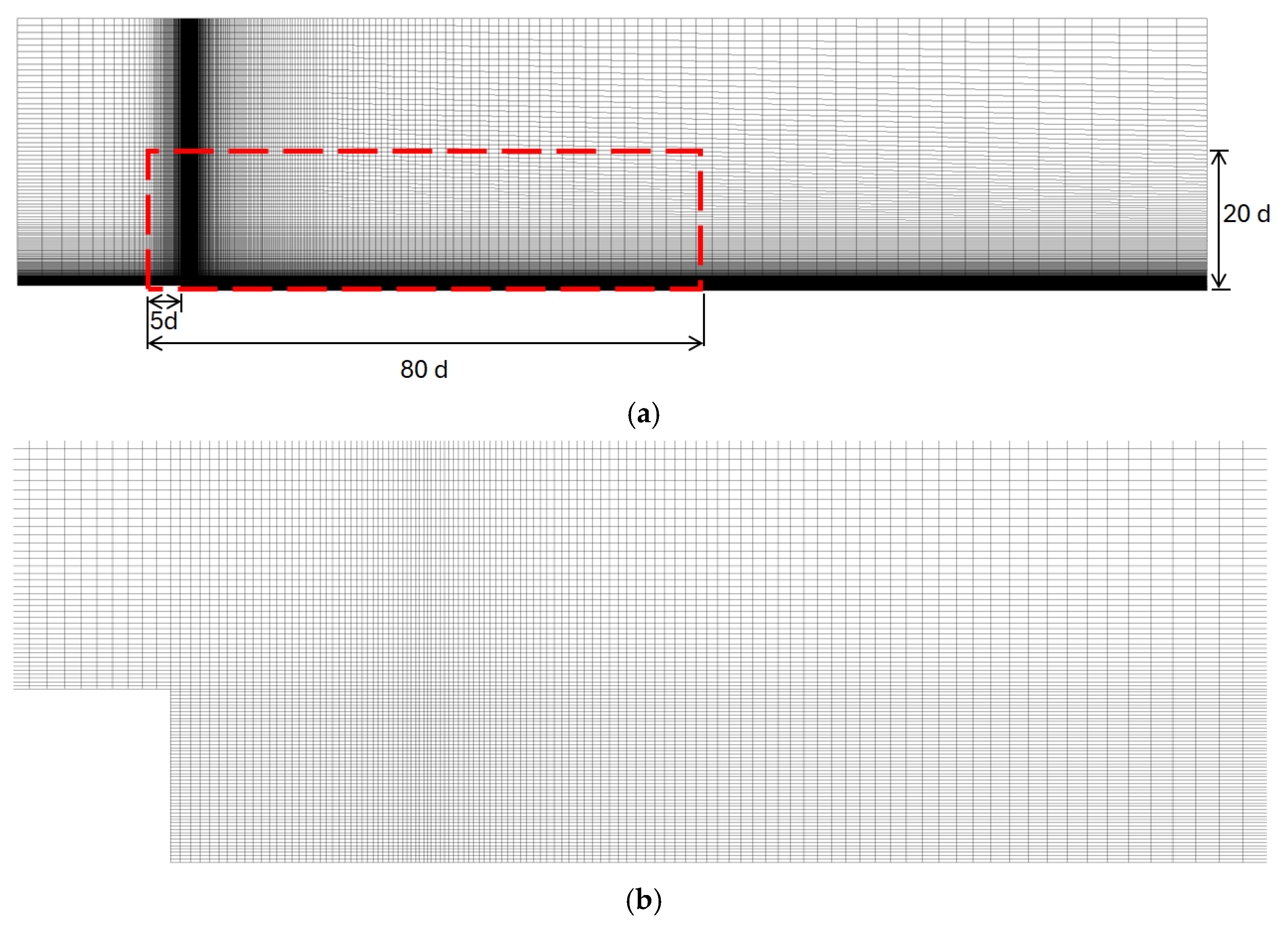
Figure 7 shows the grid used for the flame domain and its detail view for the nozzle inlet region. For clarity, in presenting the results as contour plots, the results will be shown not in the whole computational domain, but a sub-domain with an axial extension of 80 d and radial extension of 20 d, as indicated by the red rectangle with broken lines in Figure 7a.
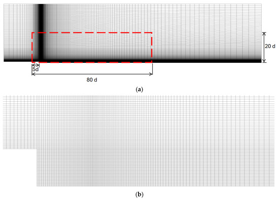
Figure 7.
Grid for flame domain: (a) complete view with indication of the region used for contour plots, (b) detail view near nozzle inlet.
7. Results for Nozzle Flow
As discussed above, the purpose of the analysis of the nozzle flow has been the derivation of detailed and consistent sets of inlet boundary conditions for the flame calculations. The calculations are carried out using the SST turbulence model, for the cases summarized in Table 1.
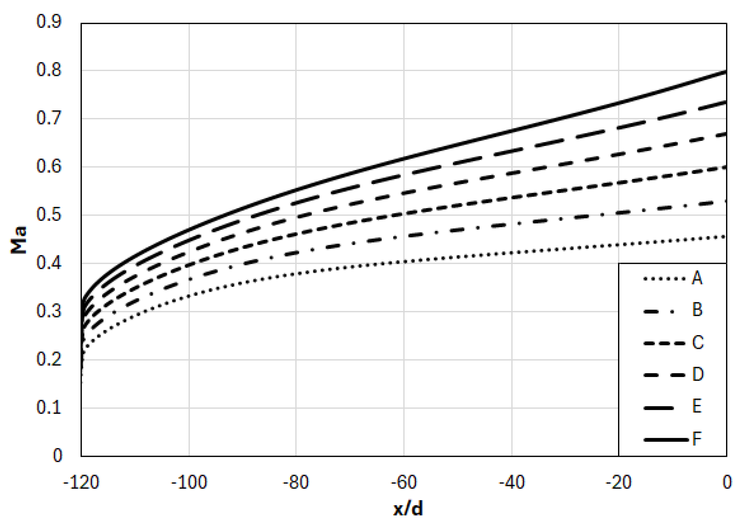
The predicted variations in the Mach number along the centerline for the considered cases (Table 1) are plotted in Figure 8. One can see that the flow experiences a substantial acceleration along the nozzle length. The centerline Mach numbers at the nozzle exit are considerably high and vary approx. between 0.45 (Case A) and 0.80 (Case F).
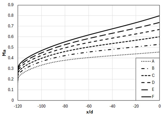
Figure 8.
Variation in Mach number along nozzle tube centerline.
As can be deduced from Figure 8, there are considerable differences between the inlet and outlet velocities of the nozzle. The nozzle outlet velocities (U) are presented in Table 1. The predicted velocities at the nozzle inlet are denoted as Uinlet (U and Uinlet are the area-averaged axial velocities at the corresponding nozzle cross sections). The differences between the nozzle outlet and inlet velocities, defined as ΔU = U-Uinlet, are listed in Table 2, where the percentage deviations are also given.
Table 2.
Differences and percentage deviations between the nozzle inlet and outlet velocities.
The predicted radial profiles of axial velocity at the nozzle exit are presented in Figure 9, for the considered six cases (Table 1). For comparison, the parabolic velocity profile for the fully developed laminar pipe flow is also displayed. One can see that the case with the lowest nozzle velocity (Case A) attains a velocity profile that is not identical with but close to the parabolic curve. With the increasing nozzle velocity, the deviation from the parabolic curve increases.
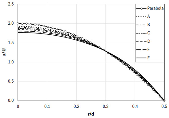
Figure 9.
Radial profiles of axial velocity at nozzle exit.
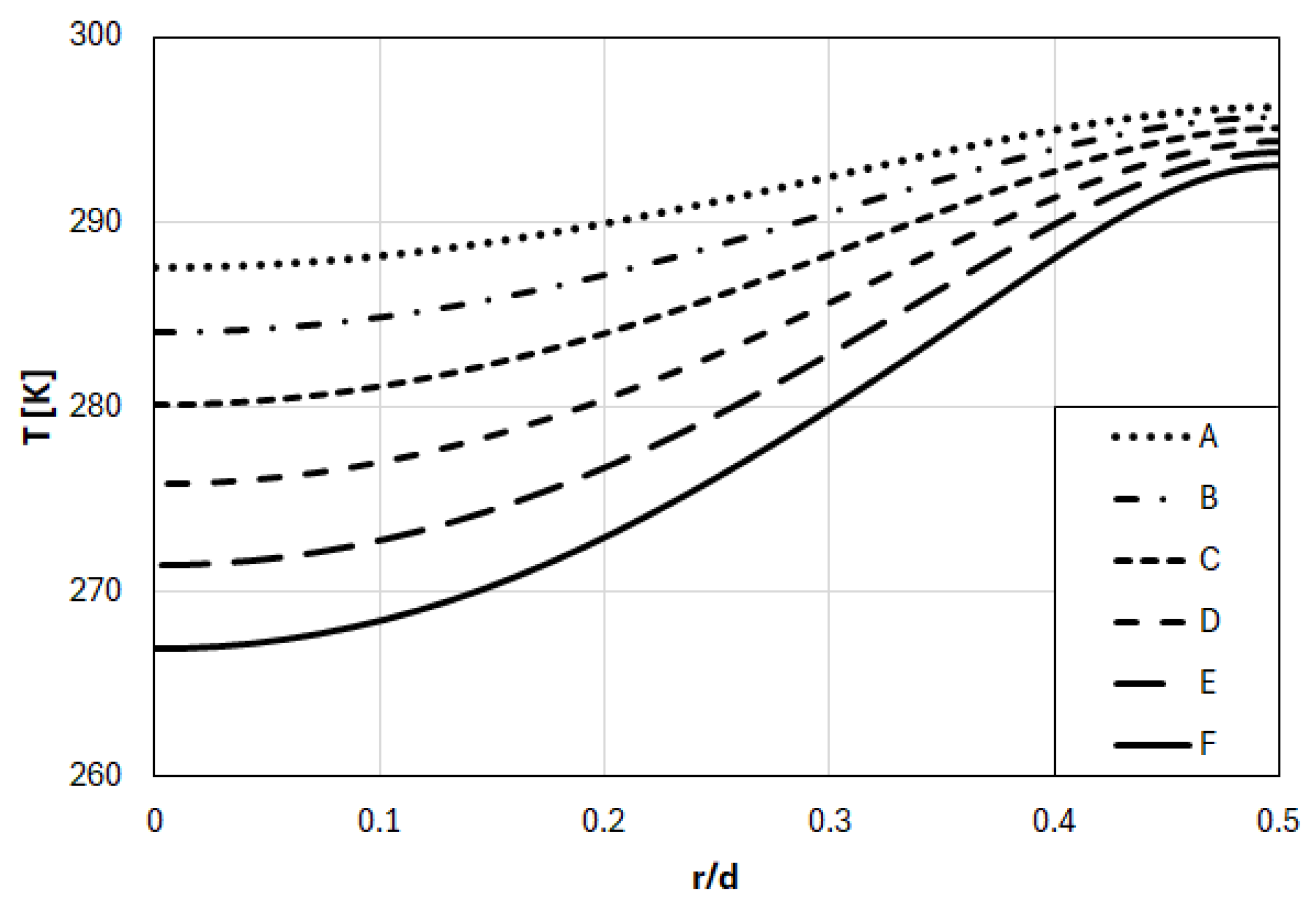
The predicted radial profiles of the static temperature at the nozzle exit are displayed in Figure 10, for the considered cases. With the increasing nozzle velocity (Mach number), the temperature decreases due to expansion.
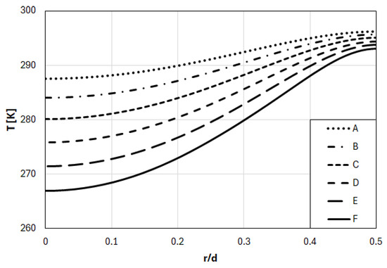
Figure 10.
Radial profiles of static temperature at nozzle exit.
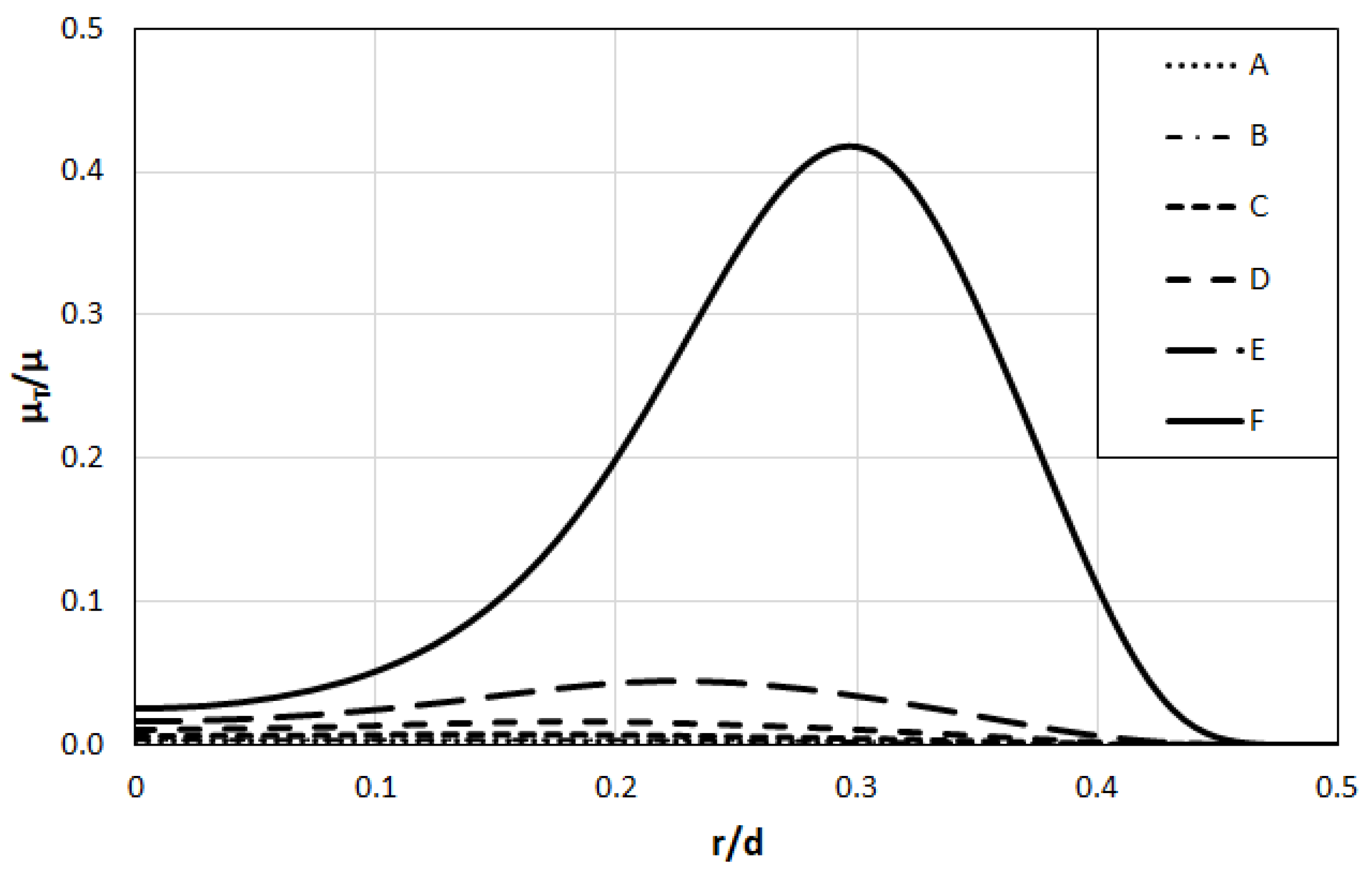
The turbulent viscosity ratio, i.e., the ratio of turbulent viscosity (μT) to the molecular viscosity (μ), can be seen as a convenient measure to judge the turbulence state of the flow. The radial profiles of the predicted turbulent viscosity ratio for the considered cases are presented in Figure 11. One can see that even for the case with the highest nozzle velocity, i.e., highest Reynolds number (Case F), the maximum value of the turbulent viscosity ratio is about 0.4, while its mean value is lower than 0.2. These very low values imply a flow state very close to the laminar flow or in a quite early stage of transition. For the other five cases (A-E), the turbulent viscosity ratios are negligibly small.
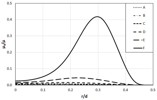
Figure 11.
Radial profiles of turbulent viscosity ratio at nozzle exit.
8. Results for Microjets in Flame Domain
In this section, the results for the microjet flames are presented for the cases summarized in Table 1.
8.1. Case A
The measured bottleneck flame shape is most predominant for Case A (Figure 2a). Thus, in the present section, this case is investigated first, where different modeling approaches are also compared and assessed.
8.1.1. Turbulence Model Assessment
As an initial step, the non-reacting flow is investigated. Predictions are obtained by the SST, T-SST and KE turbulence models. Contour plots of the turbulent viscosity ratio (μT/μ) predicted by different turbulence models are presented in Figure 12.
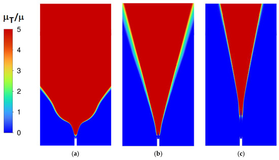
Figure 12.
Turbulent viscosity ratio for non-reacting flow for Case A: (a) KE, (b) T-SST, (c) SST.
The purpose of the present comparison is to see the prediction of the transitional behavior. Assuming that the turbulence viscosity ratio of 5 is high enough to mark the turbulent flow, the color scale is limited by 5 for a clearer display: the red regions in the figures mark the turbulent regions, whereas the blue regions are essentially the laminar zones.
For KE and T-SST, high turbulence levels are predicted immediately after the nozzle. For the SST model, the transition (marked by the condition μT/μ = 5) is predicted to occur at a distance approx. 10 d downstream from the nozzle. This seems to correlate, to an extent, with the experimentally observed downstream bottleneck position (Figure 2a).
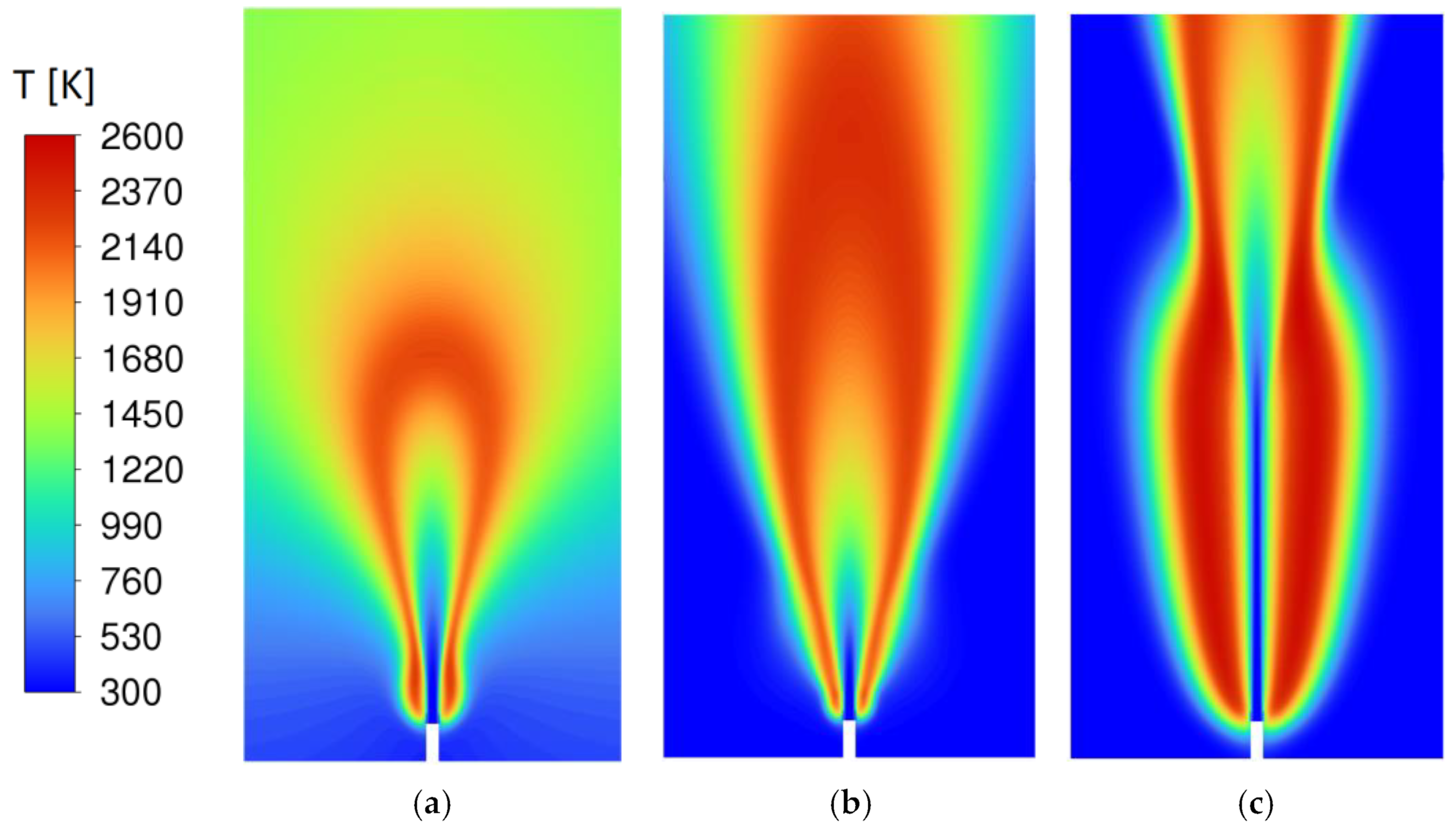
For Case A with combustion, predictions are obtained, again using the SST, T-SST and KE turbulence models, using the detailed reaction mechanism of Conaire et al. [61], and neglecting the turbulence–chemistry interactions (as mentioned above).
The flame obtained by T-SST (Figure 13b) does not show a bottleneck morphology, whereas the flame obtained by KE (Figure 13a) has only a quite weak indication of a bottleneck shape in a small region. However, the results of SST (Figure 13c) exhibit a bottleneck morphology similar to the experimental flame pattern (Figure 2a). In a relationship with the predicted turbulent viscosity ratio fields (Figure 12), this can be seen as a further indication of the correlation between the bottleneck flame shape and transition phenomena. Since, among the investigated turbulence models, only the SST seems to predict these effects (at least qualitatively), the SST model is used as the turbulence model in the further analysis.

Figure 13.
Temperature distribution for Case A: (a) KE, (b) T-SST, (c) SST.
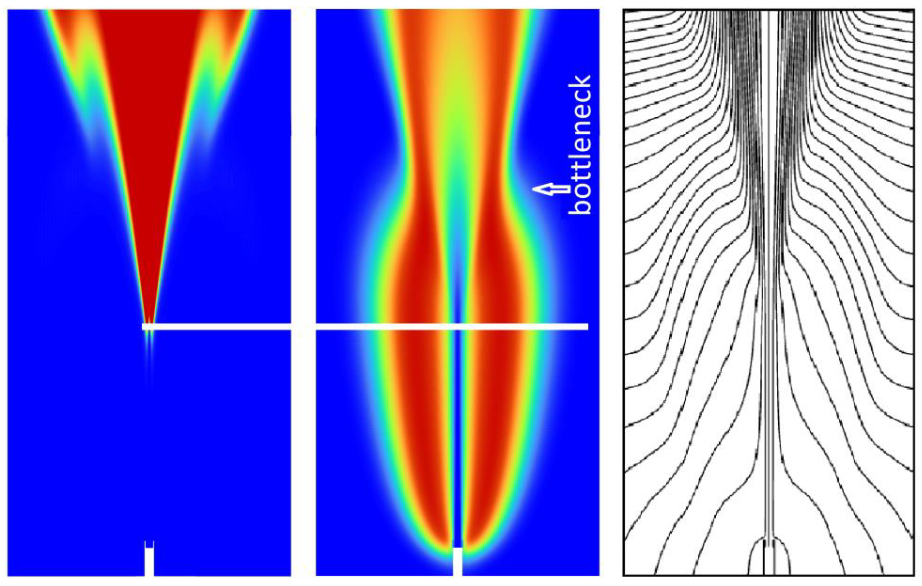
Figure 14 compares the field distributions of the turbulent viscosity ratio (scale of Figure 12) and temperature (scale of Figure 13), as well as the streamlines, for combusting Case A.

Figure 14.
Turbulent viscosity ratio (left), temperature (middle), streamlines (right) for Case A.
Compared to the non-reacting case (Figure 12c), the transition takes place at a farther downstream position, when there is combustion (Figure 14 left). The white horizontal line in Figure 14 (located at an axial distance x/d = 31 from the nozzle) is drawn to indicate the relative position of the transition point in comparison to the flame shape. It is interesting to note that the bottleneck location does not coincide with the transition point but occurs at a downstream position. The transition point roughly corresponds to the position where the bubble (bottle) has attained its largest radial expansion. This makes approximately 2/3 of the distance between the nozzle and the bottleneck. Thereafter (after transition), the bottle size starts to decrease to its minimum at the bottleneck. Looking at the streamlines, it can be seen that the flow pattern resembles that of a turbulent free jet emanating from the transition point. The bottleneck appears to occur at the intersection of the jet boundaries with the converging bottle contour.
8.1.2. Effect of Buoyancy
For assessing the effect of buoyancy, calculations are carried out by neglecting gravity. The predicted temperature field is shown in Figure 15.
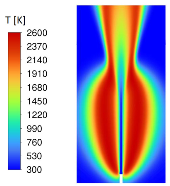
Figure 15.
Temperature distribution predicted by neglecting buoyancy, Case A.
Comparing Figure 15 with Figure 13c, one can see that a radially larger bottle is predicted, when buoyancy is neglected, while the bottleneck position also moves upstream. For macroscopic vertical free jet flames of hydrocarbon fuels, Fr > 5 was identified as the momentum-dominated range [41]. In the present case, with a considerably larger Froude number (13.5, Table 1), a notable effect of buoyancy especially on the radial expansion of the flame is still observed. The remaining cases (B to F) have larger Froude numbers (Table 1). Therefore, the effect of buoyancy is expected to be less important for them. The significance of buoyancy would decrease with the increasing Froude number.
8.1.3. Effect of Thermal Diffusion and Preferential/Differential Diffusion
The effect of thermal diffusion is investigated by performing a calculation by its omission. In hydrogen flames, it is known that differential and preferential diffusion play an important role. For finding out their effect on the bottleneck phenomenon, a calculation is also performed by neglecting them, assuming a Lewis number (Le) of unity.
The predicted temperature fields by neglecting thermal diffusion and assuming Le = 1 are presented in Figure 16.

Figure 16.
Temperature distribution for Case A: (a) thermal diffusion neglected, (b) Le = 1 assumed.
Comparing Figure 16a with Figure 13c, one can see that thermal diffusion has a rather marginal effect on the flame shape. Neglecting thermal diffusion, the flame radial extension is slightly reduced, while the bottleneck position remains rather unaffected. A much stronger change in the flame morphology is observed by the assumption of Le = 1 (Figure 16b). In a hydrogen–air flame, the Lewis number of hydrogen can be estimated to be about 0.3 [64]. Thus, the assumption of Le = 1 implies an artificial reduction in the diffusion coefficient of hydrogen by a factor of about 3 or more. Consequently, this results in an underprediction of the spatial extension of the reaction zone in all directions. Here, the radial flame size is considerably reduced. This is accompanied by a shortening of the bottle size in the axial direction and a corresponding upstream shift of the bottleneck position. Although its position is shifted, the bottleneck morphology is still observed, confirming that the phenomenon itself is not merely a result of the unique diffusion properties of hydrogen.
8.1.4. Assessment of Combustion Mechanisms and Turbulent Combustion Models
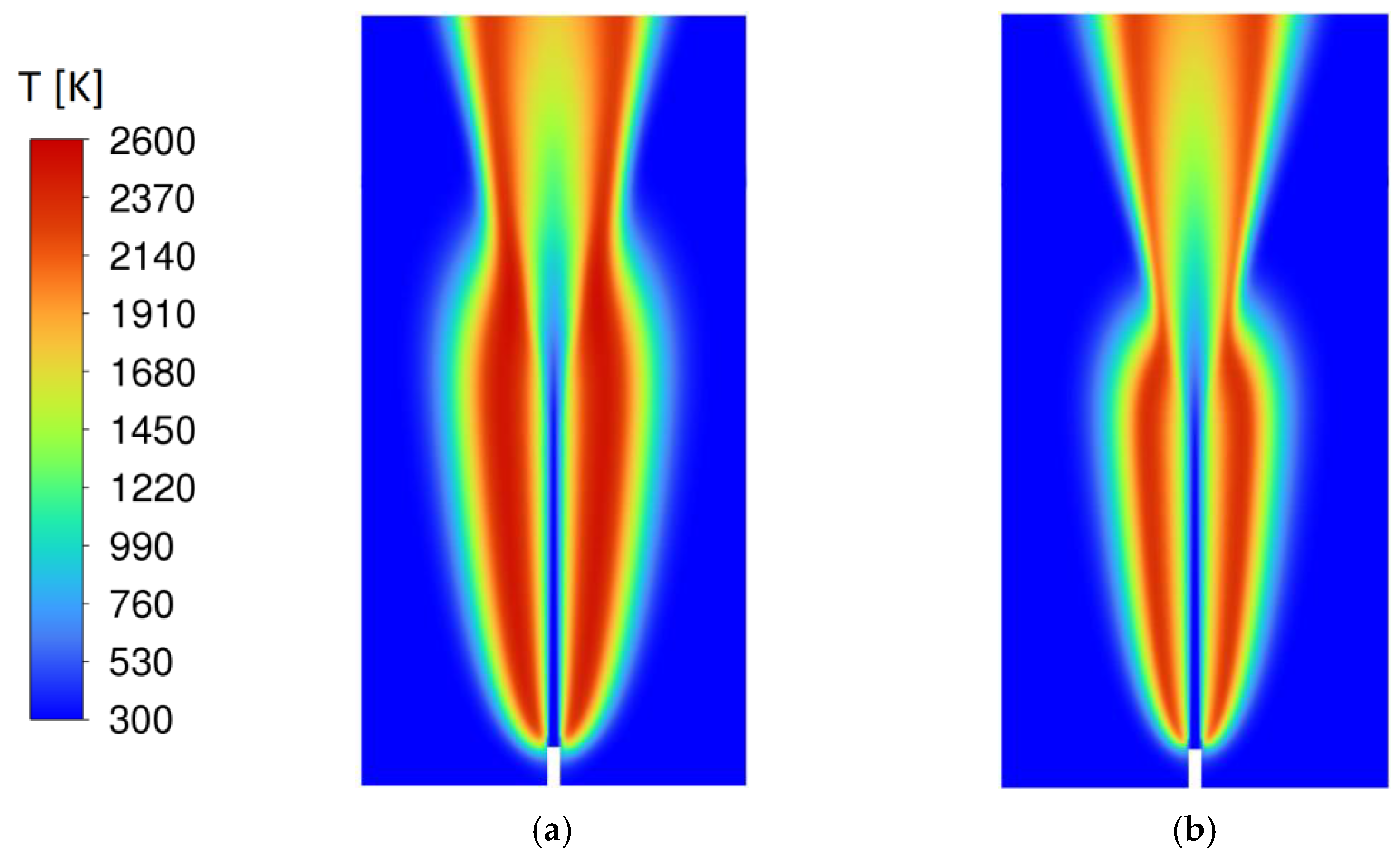
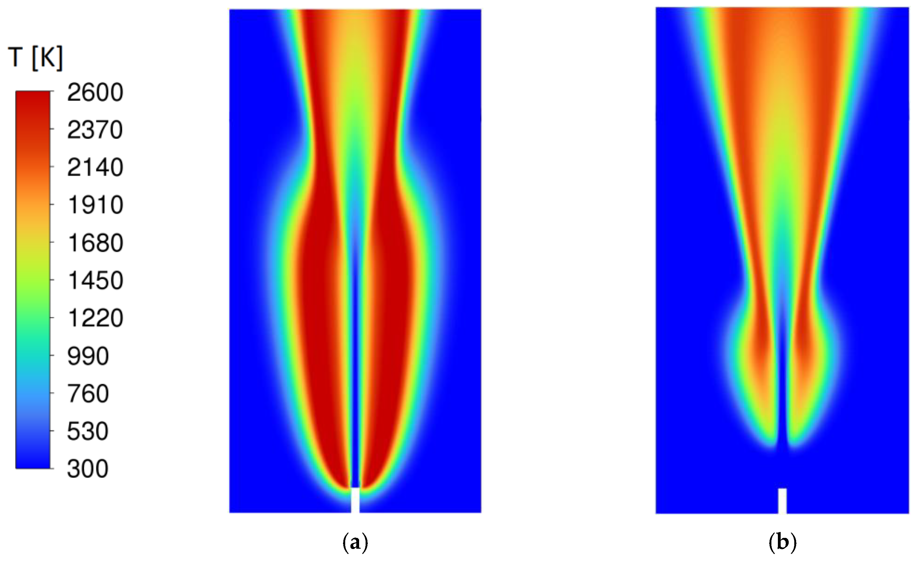
In all calculations presented above, the detailed hydrogen reaction mechanism of Conaire et al. [61] has been used. In the present section, the predictive capability of the single-step global reaction mechanism of Marinov et al. [60] is assessed. The predicted temperature distribution using the global mechanism of Marinov et al. [60] is shown in Figure 17a. Comparing Figure 17a with Figure 13c, one can see that the predicted flame morphology is practically identical. As one would expect, the predicted temperatures by the global reaction mechanism (Figure 17a) are higher compared to those of the detailed reaction mechanism (Figure 13c). However, the flame shape and the position of the bottleneck are practically identical between both reaction mechanisms.
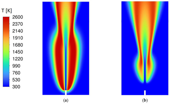
Figure 17.
Temperature field for Case A: (a) global reaction mechanism, no-model approach for turbulent combustion model, (b) detailed reaction mechanism, EDC as turbulent combustion model.
In the calculations above, for turbulent combustion, the no-model approach has been used, i.e., the turbulence–chemistry interactions have been neglected. For comparison, the Eddy Dissipation Concept (EDC) [39,62] is also applied here as the turbulent combustion model. The predicted temperature field by the EDC is presented in Figure 17b.
It can be seen in Figure 17b that a lifted flame is predicted by the EDC, where the reaction zones in the nearfield of the nozzle are predicted to be extinguished. It is also interesting to note that the bottleneck pattern is still observed in the EDC prediction, however, at a more upstream position. For the lifted flame of EDC, the transition to turbulence occurs earlier compared to the attached flame of the no-model approach (Figure 14 left) (rather similar to the non-reacting flow (Figure 12c)), which is the main reason for the more upstream position of the bottleneck in the EDC prediction.
8.2. All Cases, Comparison with Experiments
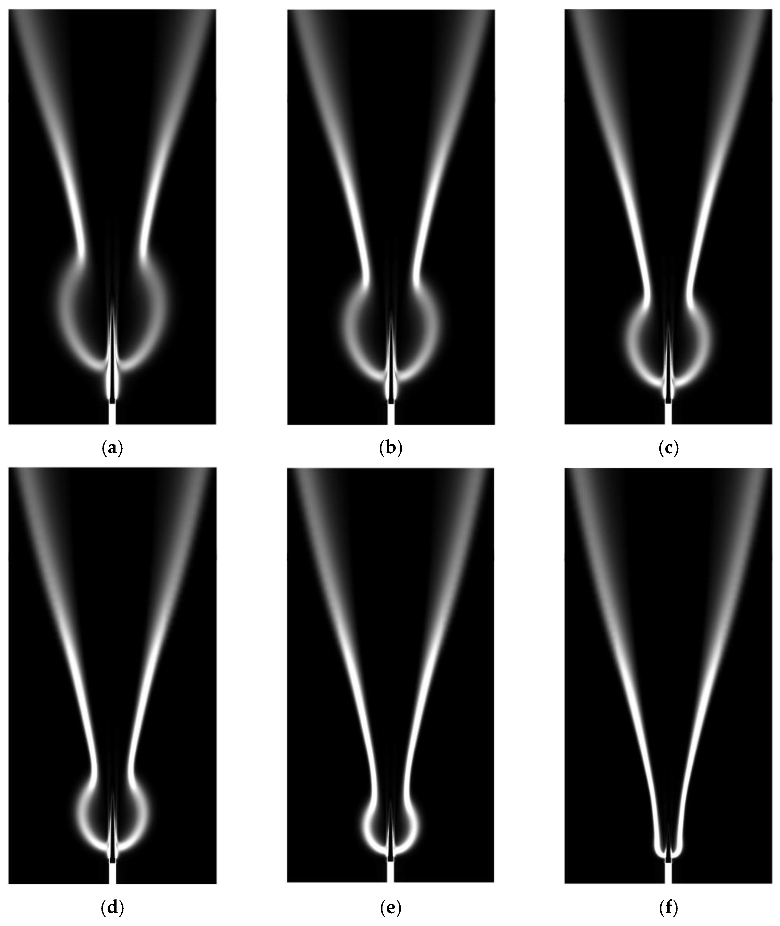
It is shown in the preceding section that the flame morphology predicted by the global [60] and detailed [61] mechanisms does not show a notable difference. Thus, the global reaction mechanism [60] is used for the calculations presented in the current section. The experimental results were presented as shadowgraphs that reveal density variations (Figure 2, [20]). Obviously, density variations are strongly coupled with temperature variations. However, variations in composition additionally play a role, especially in the present case, with large differences in the molecular masses of the components and preferential/differential diffusion, and pressure differences can also contribute. Thus, for increasing the resemblance to the displayed experimental fields, the predicted flame morphologies are displayed via the amount of the density gradient (Δρ), which is calculated from Δρ = [(∂ρ/∂x)2 + (∂ρ/∂y)2]1/2. For simplicity, the resulting fields will be referred to as Schlieren images in the following. In all field plots, the scale of Δρ is kept constant between 0 and 1000 kg/m4. Since it is about a qualitative comparison of the morphologies, scales are not provided in the figures.
The predicted Schlieren images for all considered six cases (Table 1) obtained by adopting the no-model approach for turbulent combustion are provided in Figure 18.
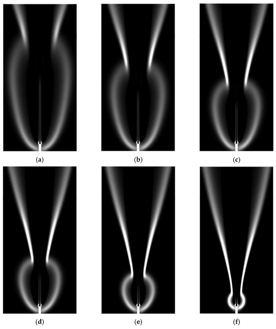
Figure 18.
Predicted Schlieren images of the considered flames (no-model approach for turbulent combustion): (a) Case A, (b) Case B, (c) Case C, (d) Case D, (e) Case E, (f) Case F.
Comparing Figure 18 with Figure 2, one can see that the predicted flame morphologies show a quite good qualitative agreement with the measurements. Similar to the experiments (Figure 2), the predictions show that the “bottle” becomes smaller and the bottleneck position moves closer to the nozzle as the nozzle velocity is increased.
The predicted Schlieren images obtained by using the EDC as the turbulent combustion model are presented in Figure 19.
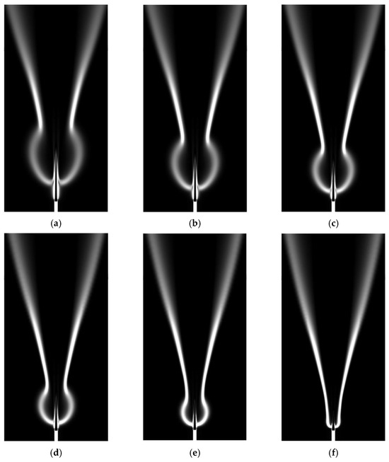
Figure 19.
Predicted Schlieren images of the considered flames (EDC for turbulent combustion): (a) Case A, (b) Case B, (c) Case C, (d) Case D, (e) Case E, (f) Case F.
The EDC results (Figure 19) also show, in general, a qualitative agreement with the measurements (Figure 2) for the bottleneck morphology. However, for Case F, no bottleneck is predicted (Figure 19f). As was previously observed in Figure 17, the bottleneck positions are predicted at more upstream positions by the EDC, compared to the no-model approach (Figure 18). It has already been observed in Figure 17b, for Case A, that the prediction by the EDC in the nozzle nearfield is inaccurate, as a lifted flame is predicted by the EDC. In Figure 19, it can be seen that a lifted flame is predicted by the EDC for all considered cases.
In the present predictions (Figure 18 and Figure 19) and in the experiments (Figure 2, [20]), a decrease in the bottle size with the increasing nozzle velocity is observed. This is expected to be mainly due to the increasing velocity gradients between the jet and environment. With the increasing nozzle velocity, the contribution of the gradients to turbulence production increases, which triggers an earlier transition.
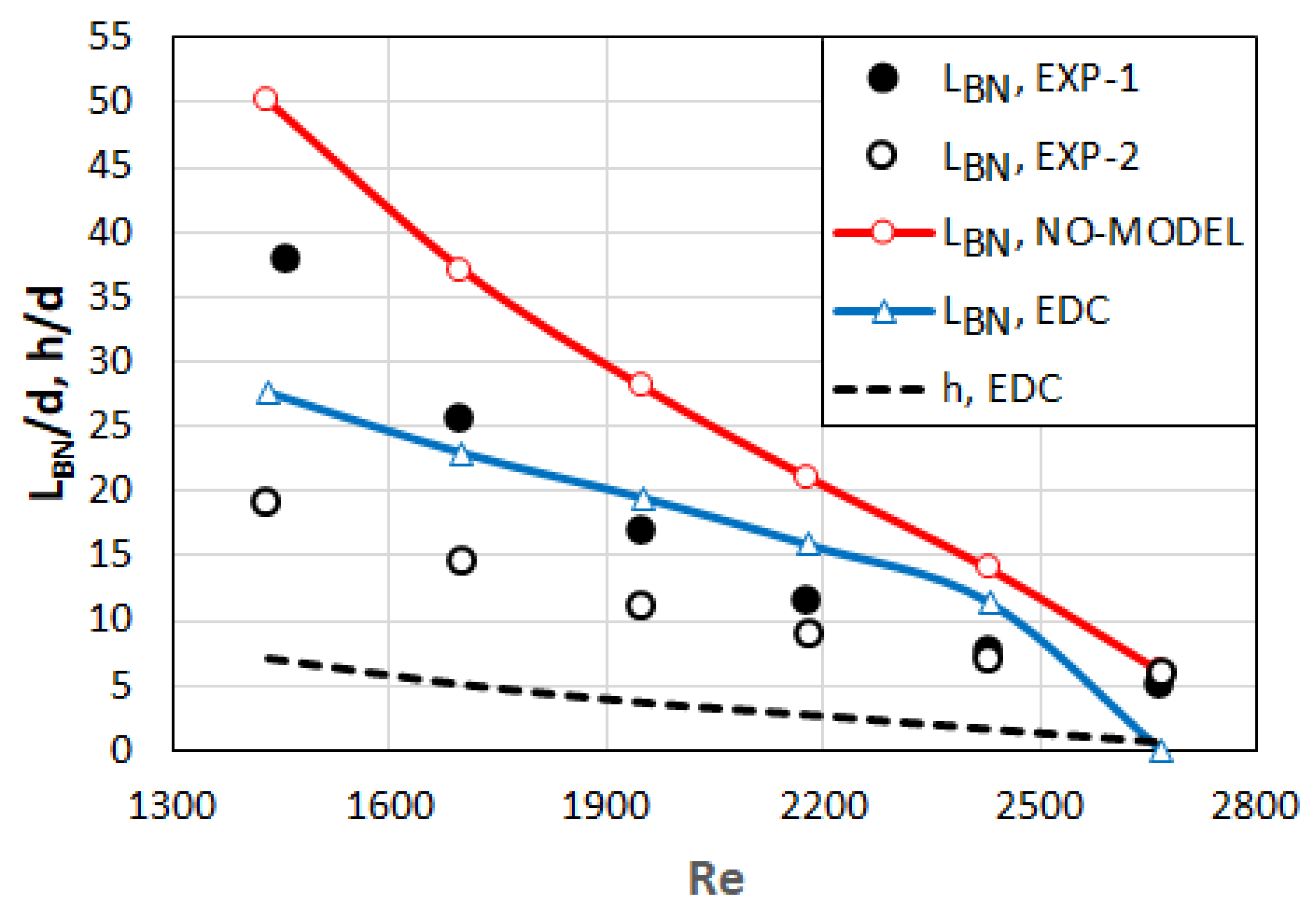
The measured [20] and predicted normalized bottleneck positions (LBN/d) (bottleneck distance measured from the nozzle outlet LBN, normalized by the nozzle diameter d) are provided in Figure 20 for all considered cases (predictions by neglecting turbulence–chemistry interactions are referred to as NO-MODEL, predictions using EDC as turbulence combustion model are referred to as EDC). At this stage, an apparent inconsistency in the presentation of the experimental results shall be addressed [20]. In addition to the shadowgraphs of flames (Figure 2), a curve plot showing the variation in LBN/d from case to case was also provided [20]. It appears that the results implied by the shadowgraphs and the curve plot do not coincide. In this respect, it shall also be acknowledged that the optical determination of the bottleneck position may be subject to some uncertainty and even subjectivity, when also considering the role of turbulent fluctuations. In the present comparison, both representations of the experimental results are considered. The results implied by the shadowgraphs of Ref. [20] are indicated by EXP-1 and the results presented in the curve plot of Ref. [20] are indicated by EXP-2. The lift-off height (h) predicted by the EDC is also displayed in the figure (in agreement with the previous work [32,36,37] in determining the lift-off height, it is assumed that the flame root is marked by an OH mole fraction of 600 ppm or by a temperature of 750 K that corresponds to this value).
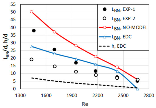
Figure 20.
Bottleneck position (LBN) and lift-off height (h) as function of Reynolds number (Re) for considered cases (Table 1).
As seen in Figure 20, both predictions (no-model and EDC) indicate a reduction in LBN with the increasing nozzle speed, and so far, agree qualitatively well with the experiments. For Re = 2670, the prediction by the no-model approach shows a perfect agreement with the experiments, whereas the EDC does not predict any bottleneck morphology (LBN = 0 is used for this case, in Figure 21).
Figure 21.
Bottleneck position (LBN) and lift-off height (h) as function of Reynolds number (Re) for considered cases (Table 1). Predictions are obtained by turbulent viscosity modification.
For Re ≤ 2430, the no-model approach overpredicts the experimental results throughout. The EDC overpredicts the EXP-2 curve for all Re. Comparing the EDC curve with the EXP-1 curve, an overprediction and underprediction are observed for Re ≤ 2180 and Re ≥ 2430, respectively, while the agreement for 2180 < Re < 2430 is quite good. The lift-off height predicted by the EDC increases with the decreasing nozzle velocity. Obviously, this is not a physically correct behavior, but just due to the inability of the model to predict combustion in laminar regimes.
From the above discussions, it becomes clear that the predictability of the transitional behavior, i.e., turbulence modeling, plays the most predominant role in the relationship with the prediction of the bottleneck flame morphology. Better results can be expected if turbulence models can be improved to predict transition in free shear layers more accurately. Here, a very simple, ad hoc attempt is taken for a turbulence model modification, by modifying the turbulent viscosity for Cases A–E. The modified viscosity (μT,MOD) is obtained by multiplying the turbulent viscosity (μT) of the SST model by a coefficient C as
and C is adjusted to fit to the experimental results. For this purpose, the experimental results presented in the line graph of Ref. [20] are taken as the reference (EXP-2)
In combination with the no-model approach, the following expression can be suggested for the coefficient,
which delivers values varying between 1.59 and 1.44 for C in the considered range.
In relationship with the EDC, the below relationship can be used
leading to C values from 1.16 to 1.22 in the considered range.
The bottleneck distances and lift-off heights (for the EDC) calculated with the above modifications are displayed in Figure 21.
One can see that a nearly perfect agreement with the measurements can be obtained by applying the above modifications of the turbulent viscosity. It is obvious that the above-mentioned ad hoc modification has no theoretical basis and can in no means claim to be universal. It is intended only for demonstrating the effect of a turbulence model modification and, hopefully, encouraging model improvements in the present context.
9. Conclusions
A computational analysis of high-speed microjet hydrogen–air diffusion flames with emphasis on the predictability of the bottleneck morphology is presented. The results are compared with the measurements of Kozlov et al. [20]. For the quantitative assessment of the prediction of the bottleneck position, two sets of experimental representations, based on the shadowgraph images and the curve plot provided in Ref. [20], are taken as the reference.
Calculations confirm that although agents such as preferential and differential diffusion may have a substantial influence on the flame shape, it is the transition to turbulence that predominantly controls the occurrence of the bottleneck morphology. At the same time, the transitional turbulence constitutes the main challenge in the prediction of this class of flames, since the available turbulence and turbulent combustion models are designed essentially for a fully turbulent flow regime. In comparison to alternative turbulent viscosity models, the SST model is found to predict the transitional behavior of the free jet qualitatively and is used as the turbulence model. For the reaction mechanism, it is observed that the use of a single-step global [60] or a detailed [61] reaction mechanism does not make a noticeable difference for the prediction of the flame shape and the bottleneck phenomenon.
As far as the turbulent combustion modeling is concerned, it is found that the flame shape can be predicted qualitatively quite well, when turbulence–chemistry interactions are neglected (no-model approach). Quantitatively, although the bottleneck position is predicted exactly for Re = 2670 by the no-model approach, an overprediction for lower Reynolds numbers is observed (in comparison to both sets of experimental results).
Using the EDC as the turbulent combustion model, no bottleneck pattern is predicted for Re = 2670. For lower Reynolds numbers, the EDC curve also overpredicts one of the experimental curves (shadowgraph-based) throughout and crosses the other one (curve plot-based), with a higher quantitative agreement. Quantitatively seen, the EDC curve is closer to the experimental curves than the no-model curve for Re ≤ 2430.
A characteristic of the EDC results is the prediction of an “artificially” lifted flame with an increasing lift-off height with a decreasing Reynolds number due to the model limitation.
It is demonstrated that a good agreement with the experiments for the bottleneck position can be obtained for 1430 ≤ Re ≤ 2430 by modifying the turbulent viscosity.
As potential future work, an analysis of the flames by the unsteady, three-dimensional, turbulence-resolving approaches such as Large Eddy Simulations is envisaged. The present study highlights the need for improved RANS models for the transition to turbulence in free shear layers, which also points out an interesting area for future research.
Funding
This research received no external funding.
Institutional Review Board Statement
Not applicable.
Informed Consent Statement
Not applicable.
Data Availability Statement
The data presented in this study may be made available on request.
Conflicts of Interest
The author declares no conflicts of interest.
References
- Sorensen, B. Renewable Energy; Academic Press: Cambridge, MA, USA, 2017. [Google Scholar]
- Radovanovic, M. Sustainable Energy Management; Academic Press: Cambridge, MA, USA, 2022. [Google Scholar]
- DuBois, E.; Mercier, A. Energy Recovery; Nova Science: Hauppauge, NY, USA, 2010. [Google Scholar]
- Benim, A.C.; Epple, B.; Krohmer, B. Modelling of pulverised coal combustion by a Eulerian-Eulerian two-phase flow formulation. Prog. Comput. Dyn. Int. J. 2005, 5, 345–361. [Google Scholar] [CrossRef]
- Barnes, I.D. Understanding pulverised coal, biomass and waste combustion e a brief overview. Appl. Therm. Eng. 2005, 74, 89–95. [Google Scholar] [CrossRef]
- Higman, C.; van der Burgt, M. Gasification, 2nd ed.; Gulf Professional Publishing: Houston, TX, USA, 2008. [Google Scholar]
- Sarker, T.R.; Nanda, S.; Dalai, A.K. Hydrogen-rich gas production from hydrothermal gasification of fuel pellets obtained fromco-pelletization of agricultural residues. Int. J. Hydrogen Energy 2024, 52, 80–93. [Google Scholar] [CrossRef]
- IAEA. Hydrogen Production Using Nuclear Energy; IAEA Nuclear Energy Series, No. NP-T-4.2; International Atomic Energy Agency: Vienna, Austria, 2013. [Google Scholar]
- Karaca, A.E.; Dincer, I.; Gu, J. Life cycle assessment study on nuclear based sustainable hydrogen production options. Int. J. Hydrogen Energy 2020, 45, 22148–22159. [Google Scholar] [CrossRef]
- Gotz, M.; Lefebvre, J.; Mors, F.; McDaniel Koch, A.; Graf, F.; Bajohr, S.; Reimert, R.; Kolb, T. Renewable power-to-gas: A technological and economic review. Renew. Energy 2016, 85, 1371–1390. [Google Scholar] [CrossRef]
- Benim, A.C.; Syed, K. Flashback Mechanisms in Lean Premixed Gas Turbine Combustion; Academic Press: Cambridge, MA, USA, 2015. [Google Scholar]
- Aniello, A.; Poinsot, T.; Selle, L.; Schuller, T. Hydrogen substitution of natural-gas in premixed burners and implications for blow-off and flashback limits. Int. J. Hydrogen Energy 2022, 47, 33067–33081. [Google Scholar] [CrossRef]
- Kudriakov, S.; Studer, E.; Bin, C. Numerical simulation of the laminar hydrogen flame in the presence of a quenching mesh. Int. J. Hydrogen Energy 2011, 26, 2555–2559. [Google Scholar] [CrossRef]
- Schönborn, A.; Sayad, P.; Klingmann, J. Influence of precessing vortex core on flame flashback in swirling hydrogen flames. Int. J. Hydrogen Energy 2014, 39, 20233–20241. [Google Scholar] [CrossRef]
- Kiymaz, T.B.; Boncu, E.; Guleryuz, D.; Karaca, M.; Yilmaz, B. Numerical investigations on flashback dynamics of premixed methane-hydrogen-air laminar flames. Int. J. Hydrogen Energy 2022, 59, 25022–25033. [Google Scholar] [CrossRef]
- Lopez-Ruiz, G.; Fernandez-Akarregi, A.R.; Diaz, L.; Urresti, I.; Alava, I.; Blanco, J.M. Numerical study of a laminar hydrogen diffusion flame based on the non-premixed finite-rate chemistry model; thermal NOx assessment. Int. J. Hydrogen Energy 2019, 44, 20426–20439. [Google Scholar] [CrossRef]
- Li, D.; Wang, R.; Yang, G.; Wan, J. Effect of hydrogen addition on the structure and stabilization of a micro-jet methane diffusion flame. Int. J. Hydrogen Energy 2021, 46, 5790–5798. [Google Scholar] [CrossRef]
- Haj Ayed, A.; Kusterer, K.; Funke, H.H.W.; Keinz, J.; Bohn, D. CFD based exploration of the dry-low-NOx hydrogen micromix combustion technology at increased energy densities. Propuls. Power Res. 2017, 6, 15–24. [Google Scholar] [CrossRef]
- You, C.-H.; Lee, H.Y.; Hwang, S.-S. Low NOX combustion characteristics by hydrogen micro jet flame in cross flow. J. Mech. Sci. Technol. 2023, 37, 445–455. [Google Scholar] [CrossRef]
- Kozlov, V.V.; Grek, G.R.; Korobeinichev, O.P.; Litvinenko, Y.A.; Shmakov, A.G. Features of diffusion combustion of hydrogen in the round and plane high-speed microjets (Part II). Int. J. Hydrogen Energy 2016, 41, 20240–20249. [Google Scholar] [CrossRef]
- Kozlov, V.V.; Grek, G.R.; Kozlov, G.V.; Litvinenko, Y.A.; Shmakov, A.G. Experimental study on diffusion combustion of high-speed hydrogen round microjets. Int. J. Hydrogen Energy 2019, 44, 457–468. [Google Scholar] [CrossRef]
- Kozlov, V.V.; Vikhorev, V.V.; Grek, G.R.; Litvinenko, Y.A.; Shmakov, A.G. Diffusion combustion of a hydrogen microjet at variations of its velocity profile and orientation of the nozzle in the field of gravitation. Combust. Sci. Technol. 2019, 191, 1219–1235. [Google Scholar] [CrossRef]
- Shmakov, A.G.; Grek, G.R.; Kozlov, V.V.; Litvienko, Y.A. Influence of initial and boundary conditions at the nozzle exit upon diffusion combustion of a hydrogen microjet. Int. J. Hydrogen Energy 2017, 42, 15913–15924. [Google Scholar] [CrossRef]
- Takahashi, F.; Mizomoto, M.; Ikai, S. Transition from laminar to turbulent free jet diffusion flames. Combust. Flame 1982, 48, 85–95. [Google Scholar] [CrossRef]
- Agarwal, A.K.; Burt, A.W.; Alammar, K.N. Effect of buoyancy on transitional hydrogen gas-jet diffusion flames. Combust. Sci. Technol. 2005, 177, 2305–2322. [Google Scholar] [CrossRef]
- Glassman, I.; Yetter, R.A.; Glumac, N.G. Combustion, 5th ed.; Academic Press: Cambridge, MA, USA, 2014. [Google Scholar]
- Libby, P.A.; Williams, F.A. Turbulent Reacting Flows, 2nd ed.; Academic Press: Cambridge, MA, USA, 1994. [Google Scholar]
- Xiao, H.; Wang, Q.; He, X.; Sun, J.; Yao, L. Experimental and numerical study on premixed hydrogen/air flame propagation in horizontal rectangular closed duct. Int. J. Hydrogen Energy 2010, 35, 1367–1376. [Google Scholar] [CrossRef]
- Kim, W.; Namba, T.; Johzaki, T.; Endo, T. Self-similar propagation of spherically expanding flames in lean hydrogen-air mixtures. Int. J. Hydrogen Energy 2020, 45, 25608–25614. [Google Scholar] [CrossRef]
- Shmakov, A.G.; Kozlov, V.N.; Litvinenko, M.V.; Litvinenko, Y.A. Effect of inert and reactive gas additives to hydrogen and air blow-off of flame at hydrogen release from microleakage. Int. J. Hydrogen Energy 2021, 46, 2796–2803. [Google Scholar] [CrossRef]
- Benim, A.C.; Pfeiffelmann, B. Computational investigation of laminar premixed hydrogen flame past a quenching mesh. Int. J. Numer. Methods Heat Fluid Flow 2020, 30, 1923–1935. [Google Scholar] [CrossRef]
- Toro, V.V.; Mokhov, A.V.; Levinsky, H.B.; Smooke, M.D. Combined experimental and computational study of laminar, axisymmetric hydrogen-air diffusion flames. Proc. Combust. Inst. 2005, 30, 485–492. [Google Scholar] [CrossRef]
- Piemsinlapakunchon, T.; Paul, M.C. Effects of content of hydrogen on the characteristics of co-flow laminar diffusion flame of hydrogen/nitrogen mixture in various flow conditions. Int. J. Hydrogen Energy 2018, 43, 3015–3033. [Google Scholar] [CrossRef]
- Skottene, M.; Rian, K.E. A study on NOx formation in hydrogen flames. Int. J. Hydrogen Energy 2007, 32, 3572–3585. [Google Scholar] [CrossRef]
- Benim, A.C.; Korucu, A. Computational investigation of non-premixed hydrogen-air laminar flames. Int. J. Hydrogen Energy 2023, 48, 14492–14510. [Google Scholar] [CrossRef]
- Benim, A.C.; Pfeiffelmann, B.; Oclon, P.; Taler, J. Computational investigation of a lifted hydrogen flame with LES and FGM. Energy 2019, 173, 1172–1181. [Google Scholar] [CrossRef]
- Benim, A.C.; Pfeiffelmann, B. Comparison of Combustion Models for Lifted Hydrogen Flames within RANS Framework. Energies 2020, 13, 152. [Google Scholar] [CrossRef]
- Funke, H.H.W.; Beckmann, N.; Keinz, J.; Abanteriba, S. A comparison of numerical combustion models for hydrogen and hydrogen-rich syngas applied for dry-low-Nox-micromix-combustion. J. Eng. Gas Turbines Power 2018, 140, 081504. [Google Scholar] [CrossRef]
- ANSYS Fuent Release 2022/R2, Theory Guide. 2022. Available online: https://www.ansys.com/products/fluids/ansys-fluent (accessed on 31 July 2024).
- Streeter, W.L.; Wylie, E.B. Fluid Mechanics, 7th ed.; McGraw-Hill: New Yor, NY, USA, 1979. [Google Scholar]
- Schefer, R.W.; Houf, W.G.; Bourne, B.; Colton, J. Spatial and radiative properties of an open-flame hydrogen plume. Int. J. Hydrogen Energy 2006, 31, 1332–1340. [Google Scholar] [CrossRef]
- Turns, S.R. An Introduction to Combustion, 3rd ed.; McGraw Hill: New York, NY, USA, 2012. [Google Scholar]
- Bird, R.B.; Stewart, W.E.; Lightfoot, E.N. Transport Phenomena, 2nd ed.; Wiley: Hoboken, NJ, USA, 2002. [Google Scholar]
- Kee, R.J.; Coltrin, M.E.; Glarborg, P.; Zhu, H. Chemically Reacting Flow, 2nd ed.; Wiley: Hoboken, NJ, USA, 2018. [Google Scholar]
- Kuo, K.K.-Y. Principles of Combustion; Wiley: Hoboken, NJ, USA, 1986. [Google Scholar]
- Özisik, M.N. Radiative Transfer and Interactions with Conduction and Convection; Wiley: Hoboken, NJ, USA, 1973. [Google Scholar]
- Hottel, H.C.; Sarofim, A.F. The effect of gas flow patterns on radiative transfer on cylindrical enclosures. Int. J. Heat Mass Transf. 1965, 8, 1153–1169. [Google Scholar] [CrossRef]
- Smith, T.F.; Shen, Z.F.; Friedman, J.N. Evaluation of coefficients for the weighted sum of gray gases model. J. Heat Transf. 1982, 104, 602–608. [Google Scholar] [CrossRef]
- Hinze, J.O. Turbulence, 2nd ed.; McGraw-Hill: New York City, NY, USA, 1975. [Google Scholar]
- Durbin, P.A.; Pettersson Reif, B.A. Statistical Theory and Modeling for Turbulent Flows; Wiley: Hoboken, NJ, USA, 2010. [Google Scholar]
- Leschziner, M. Statistical Turbulence Modelling for Fluid Dynamics, Demistified; Imperial College Press: London, UK, 2015. [Google Scholar]
- Langtry, R.B.; Menter, F.R. Correlation-based transition modeling for unstructured parallelized computational fluid dynamics codes. AIAA J. 2009, 47, 2894–2906. [Google Scholar] [CrossRef]
- Menter, F.R.; Langtry, R.B.; Likki, S.R.; Suzen, Y.B.; Huang, P.G.; Volker, S. A correlation-based transition model using local variables: Part I—Model formulation. J. Turbomach. 2006, 128, 413–422. [Google Scholar] [CrossRef]
- Langtry, R.B.; Menter, F.R.; Likki, S.R.; Suzen, Y.B.; Huang, P.G.; Volker, S. A correlation-based transition model using local variables: Part II—Test cases and industrial applications. J. Turbomach. 2006, 128, 423–434. [Google Scholar] [CrossRef]
- Benim, A.C.; Pasqualotto, E.; Suh, S.-H. Modelling turbulent flow past a circular cylinder by RANS, URANS, LES and DES. Prog. Comput. Fluid Dyn. Int. J. 2008, 8, 299–307. [Google Scholar] [CrossRef]
- Menter, F.M. Two-equation eddy-viscosity turbulence models for engineering applications. AIAA J. 1994, 32, 1598–1605. [Google Scholar] [CrossRef]
- Launder, B.E.; Spalding, D.B. The numerical computation of turbulent flows. Comput. Methods Appl. Mech. Eng. 1974, 3, 269–289. [Google Scholar] [CrossRef]
- Chen, H.C.; Patel, V.C. Near-wall turbulence models for complex flows including separation. AIAA J. 1988, 26, 641–648. [Google Scholar] [CrossRef]
- Garnier, E.; Adams, N.; Sagaut, P. Large Eddy Simulation for Compressible Flows; Springer: Berlin, Germany, 2009. [Google Scholar]
- Marinov, N.M.; Westbrook, C.K.; Pitz, W. Detailed and Global Chemical Kinetics Model for Hydrogen; Report No. UCRL-JC-120677; Lawrence Livermore National Laboratory: Livermore, CA, USA, 1995. [Google Scholar]
- Conaire, M.O.; Curran, H.J.; Simmie, J.M.; Pitz, W.J.; Westbrook, C.K. A comprehensive modeling study of hydrogen oxidation. Int. J. Chem. Kinet. 2004, 36, 603–622. [Google Scholar] [CrossRef]
- Gran, I.R.; Magnussen, B.F. A numerical study of a bluff-body stabilized diffusion flame. Part 2. Influence of combustion modeling and finite-rate chemistry. Combust. Sci. Technol. 1996, 119, 191–217. [Google Scholar] [CrossRef]
- Versteeg, H.K.; Malalasekera, W. An Introduction to Computational Fluid Dynamics—The Finite Volume Method, 2nd ed.; Pearson: London, UK, 2007. [Google Scholar]
- Pitsch, H. The transition to sustainable combustion: Hydrogen- and carbon-based future fuels and methods dealing with their challenges. Proc. Combust. Inst. 2024, 40, 105638. [Google Scholar] [CrossRef]


Disclaimer/Publisher’s Note: The statements, opinions and data contained in all publications are solely those of the individual author(s) and contributor(s) and not of MDPI and/or the editor(s). MDPI and/or the editor(s) disclaim responsibility for any injury to people or property resulting from any ideas, methods, instructions or products referred to in the content. |
© 2024 by the author. Licensee MDPI, Basel, Switzerland. This article is an open access article distributed under the terms and conditions of the Creative Commons Attribution (CC BY) license (https://creativecommons.org/licenses/by/4.0/).