The Optimization of a Ternary Blend Using Grey Relation Analysis with the Taguchi Method for the Improved Performance and Reduction of Exhaust Emissions

Abstract

The demand for renewable and environmentally friendly fuels has prompted the exploration of alternative energy sources to replace conventional fossil fuels. This work investigates the optimization of a ternary blend comprising cottonseed oil (CSO), neem oil (NO), and orange peel Oil (OPO) for improved combustion characteristics, enhanced performance, and reduced exhaust emissions. Biodiesels like Cotton Seed Oil Methyl Ester (CSOME), Neem Oil Methyl Ester (NOME), and Orange Peel Oil Methyl Ester (OPOME) were made from CSO, NO, and OPO, respectively. The experimental results show major improvements in thermal efficiency and reductions in key pollutants, including NOx, CO, HC, and smoke. The best blending ratios are determined through a methodical process that employs optimization tools such as Grey Relation Analysis (GRA) with the Taguchi Method and ANOVA for validation. Then, various proportions of these biodiesels were tested in a CRDI engine to optimize the ternary blend proportions. The addition of 10% CSO and 10% OPO to NO reduces NOx emissions by 10% at CR17 as compared to diesel. Brake thermal efficiency improved by 9.08%. HC emission decreased by 10%. Average smoke opacity decreased by 27.65%. Cylinder pressure remains unchanged, but the Net Heat Release rate increased by 2%. Optimum parameters obtained are G2B10 Blend, Load 100%, CR17 and 10% EGR. The findings underscore the potential of this ternary blend as a viable alternative to conventional diesel fuel, with GRA using Taguchi proving to be an effective optimization tool for Multi-Criteria Decision Making (MCDM).

1. Introduction

The creation of cleaner and more sustainable energy sources is required due to the depletion of fossil fuel supplies and the effects of greenhouse gas emissions on the environment. Because of their low toxicity, biodegradability, and capacity to lower harmful emissions, biofuels made from renewable feedstocks are attracting more attention [1]. Because they are readily available, inexpensive, and pose little threat to food crops, non-edible oils like cottonseed oil, neem oil, and orange peel oil stand out among these. Numerous studies have explored the potential of biofuels as alternatives to diesel fuel. For example, Knothe and Razon (2017) reviewed the properties and performance of biodiesel derived from various feedstocks, highlighting the role of optimization in achieving desired combustion and emission characteristics [1]. Ramadhas et al. (2004) emphasized the importance of feedstock selection and transesterification in producing high-quality biodiesel [2]. Kalam and Masjuki (2002) demonstrated the potential of palm oil biodiesel to reduce engine emissions while maintaining performance comparable to diesel [3]. Research on the blends of biofuels indicates significant advantages over single-feedstock biodiesel. B. Çiftçi et al. (2009) studied the combustion characteristics of waste cooking oil biodiesel blended with fusel oil, noting improved ignition properties and reduced emissions [4]. Similarly, Chauhan et al. (2013) explored the performance of jatropha biodiesel blended with mahua oil and diesel, reporting enhanced brake thermal efficiency and lower unburnt hydrocarbons. These studies underscore the benefits of blending biofuels to exploit complementary properties [5].

Ternary blends of biofuels are gaining attention due to their ability to combine the unique properties of individual oils, resulting in synergistic effects on engine performance and emissions. For instance, Jain and Sharma (2010) reported that blends of jatropha, karanja, and mahua oils exhibited superior thermal efficiency and lower emissions compared to single-source biodiesel [6]. Similarly, research conducted by Bhale et al. (2009) highlighted the improved combustion characteristics of a blend of linseed oil, mahua oil, and turpentine oil [7]. Prasad et al. (2014) explored combinations of neem oil, rice bran oil, and waste cooking oil biodiesel, demonstrating significant reductions in NOx and particulate matter emissions [8]. Gopinath Dhamodaran et al. (2016) demonstrated a comparison of neem oil, rice bran oil, and cottonseed oil biodiesel, where the degree of unsaturation is the main parameter that affects NOx emissions [9].

Despite these advancements, the optimization of ternary blends using systematic tools remains underexplored. Advanced methodologies such as the response Artificial Neural Network (ANN), surface methodology (RSM), genetic algorithms (GAs) and Grey Relation Analysis (GRA) with the Taguchi Method provide robust frameworks for identifying optimal blend ratios to maximize performance and minimize emissions. This study aims to optimize a ternary blend of cottonseed oil, neem oil, and orange peel oil to achieve improved combustion performance and reduced exhaust emissions. By leveraging Grey Relation Analysis (GRA) with the Taguchi Method optimization technique, this research provides insights into achieving a sustainable and efficient biofuel blend for compression ignition engines.

Many researchers have utilized Multi-Criteria Decision Making (MCDM) techniques, incorporating Grey Relational Analysis (GRA) combined with the Taguchi Method for optimization. Chicken methyl ester was used in blending with diesel from 0% to 20%, and GRA was used to optimize the blend% and engine speed [10]. Karnwal et al. used GRA and the Taguchi technique to optimize the injection timing, CR, nozzle-opening pressure, and the % of thumba biodiesel–diesel blend. With improved engine responses, they found the optimal solution [11]. Four input parameters—compression ratio, fuel injection timing, air temperature, and air pressure—as well as responses—brake thermal efficiency, brake specific fuel consumption, hydrocarbon emission, and smoke opacity—were investigated using the GRA and Taguchi technique [12]. Analysis of Variance (ANOVA) has been used to identify the important contributions of each parameter, and the Grey Relational Grade (GRG) has been used to identify the ideal parameter levels. Grey relational analysis can be used to maximize a number of response properties. To confirm the experimental results, ANOVA and confirmation tests were also conducted. Finer atomization and better fuel-air mixing are made possible by OPO’s significantly lower kinematic viscosity compared to diesel and other fuels. It encourages evaporation and combustion because its flash and boiling points are lower than those of diesel fuel. Lemon peel oil’s natural oxygen concentration may also promote full combustion and reduce the emissions of CO and HC. OPO has lower H% and C% than diesel, which results in lower CO and HC levels. Orange peel oil has a flash point of 68 °C, meaning that fuels with a value of more than 65 °C are safe to handle and store. Orange peel oil is therefore superior to diesel in terms of safety [13].

2. Materials and Methods

2.1. Feedstock Selection

To make CSOME, cotton (Gossypium arboreum) is grown in Maharashtra, Madhya Pradesh, and Gujarat. It produces 14.71 q/ha of seed cotton and is ready in 160 days [14]. NOME is made from neem seeds (Azadirachta indica), which are grown in Rajasthan, Tamil Nadu, and Uttar Pradesh. Moreover, OPOME is made from orange peels in states like Maharashtra, Madhya Pradesh, and Tamil Nadu that grow citrus fruits. Pilot studies on ternary mixes of CSOME, NOME, and OPOME demonstrated enhanced BTE and lower emissions for the B20 blend when compared to diesel, confirming their suitability. Feedstocks were chosen based on their availability, physicochemical characteristics, and suitability for diesel engines. CSOME improves combustion by providing high calorific value, improved cetane number, and strong oxidative stability [15]. Because NOME is oxygen-rich and inedible, its high cetane number increases combustion efficiency [16]. OPOME contributes to improved atomization and igniting properties because of its low density, high volatility, and limonene concentration [17]. Neem fruits, cottonseeds, and orange peels were gathered, dried, and processed to eliminate moisture. Methanol and a KOH catalyst were used to transesterify-extracted oils at 60 °C in an 8:1 molar ratio. OPOME involved extracting oil from orange peel waste prior to transesterification, and purification was then performed to obtain the final methyl esters.

Testing fuel was prepared using three biodiesels such as CSO, NO, OPO in three proportions of CSO: NO: OPO as 8:1:1, 1:8:1, 1:1:8, named as G1, G2 and G3, respectively. So, G1 is the group in which cottonseed oil dominates the other two oils, in G2, neem oil dominates the other two oils, and, in G3, OPO dominates the other two oils, as shown in Figure 1.

After finalizing, the proportion of pure biodiesel was prepared using the transesterification process to reduce the density and viscosity of oils [18,19,20]. After 100% biodiesel preparation, blends of these hybrid biodiesel are prepared with diesel. G1B10 indicates 10% biodiesel from G1 and 90% diesel, G2B10 indicates 10% biodiesel from G2 and 90% diesel, and G3B10 is 10% biodiesel from G3 and 90% diesel.

Table 1. Properties of testing fuel.

Sr. No	Test Description	Ref Std ASTM 6751	Reference		Testing Fuel
			Unit	Limit	B00	G1B10	G2B10	G3B10
1	Density	D1448	gm/cc	0.800–0.900	0.832	0.835	0.836	0.836
2	Calorific Value	D6751	MJ/Kg	34–45	42.7	42.11	42	42.26
3	Cetane Number	D613	NA	41–55	49	49.6	49.55	49.6
4	Viscosity	D445	mm2/s	3–6	2.7	4.65	4.87	3.98
5	Flash Point	D93	°C	-	64	160	149	83
6	Fire Point	D93	°C	-	72	160	170	140
7	Moisture	D2709	%	0.05%	Nil	Nil	Nil	Nil

, showing various instruments, was used to measure the density, viscosity, calorific value, cetane number, and flash point of the testing fuels.

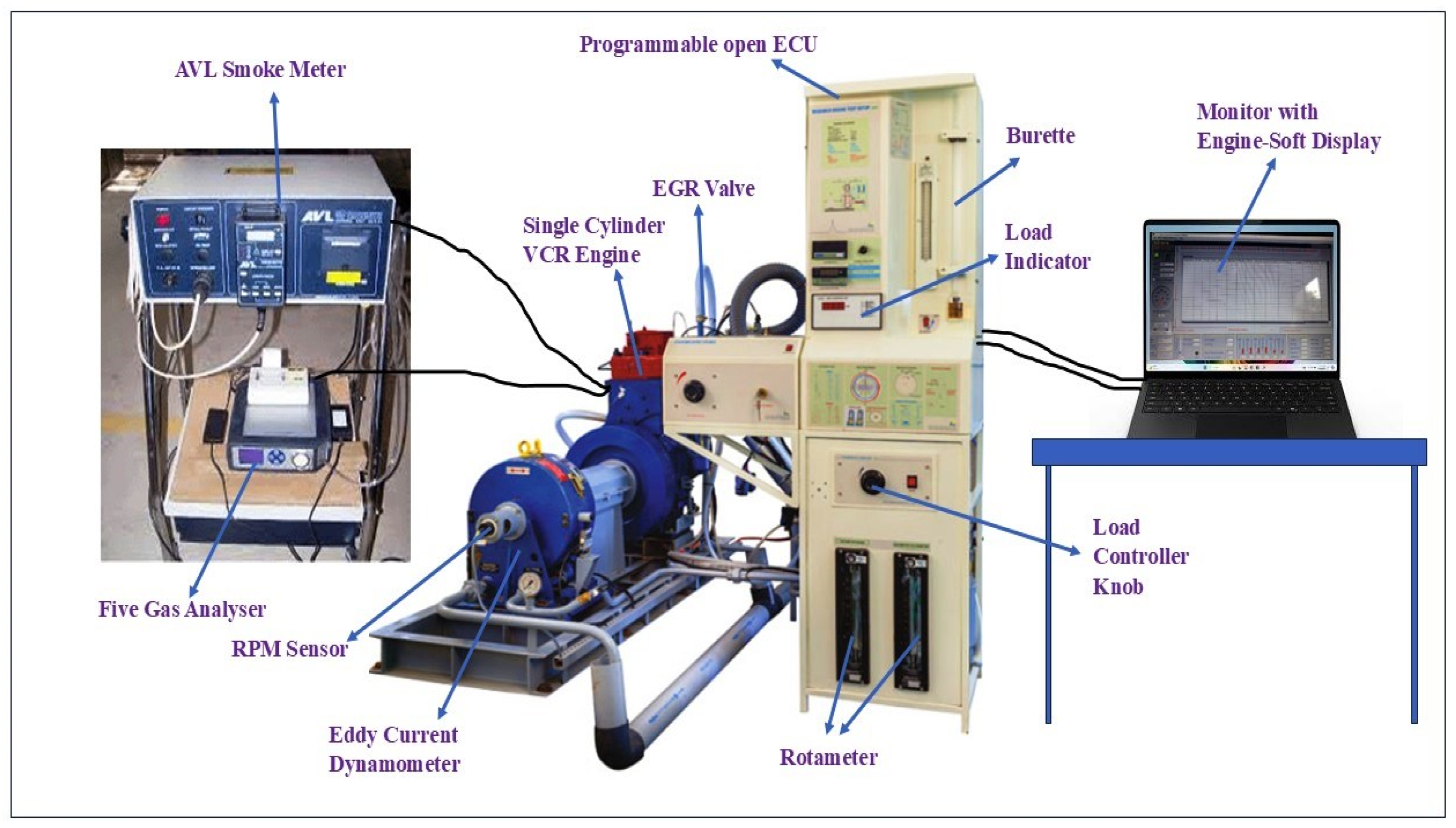
2.2. Experimental Setup and Measurements

Figure 2 depicts the engine setup, which was a computerized CRDI VCR Engine test built by Kirloskar and had a single cylinder, four strokes, water-cooling, a stroke of 110 mm, a bore of 87.5 mm, and a displacement of 661 cc with a CR range of 12–18, and an output of 3.5 kW at 1500 rpm. An air box, twin fuel tanks, a manometer, fuel measurement units, fuel and air flow transmitters, calorimeters, water flow metres, and cooling rotameters were additional parts of the system. These devices measure temperature, load, crank angle, combustion pressure, airflow, fuel flow, and airflow. The engine’s programmable ECU controls the injection, common rail, pressure sensor, fuel pump, and compression ratio by tilting the cylinder block. This setup allows you to study engine characteristics such as brake power, thermal efficiency, and fuel consumption at different compression ratios and EGR levels. The exhaust gases were tested using a five-gas analyzer (CO, HC, CO₂, O₂, and NOx), and the smoke opacity was measured with an AVL smoke metre. Apex Innovations developed Engine Soft; a Lab view-based tool for real-time performance monitoring that includes data gathering, analysis, and export capabilities compatible with Excel.

Table 2. Details of emission measurement instruments and procedures.

Emission Parameter	Instrument Used	Measurement Principle	Calibration Method	Measurement Range	Resolution
Nitrogen Oxides (NOxs)	Chemiluminescence NOx Analyzer (Horiba PG-250)	Chemiluminescence Detection (CLD)	Zero calibration (N2), span calibration (NO2 in N2)	0–5000 ppm	±1 ppm
Hydrocarbons (HCs)	Flame Ionization Detector (FID) Gas Analyzer (AVL 444)	Flame Ionization Detection	Propane gas in balance air	0–10,000 ppm	±0.1 ppm
Carbon Monoxide (CO)	Non-Dispersive Infrared (NDIR) Gas Analyzer (Testo 350)	Infrared Absorption	Zero calibration (N2), span calibration (CO in N2)	0–10%	±0.01%
Carbon Dioxide (CO2)	Non-Dispersive Infrared (NDIR) Gas Analyzer (Testo 350)	Infrared Absorption	Zero calibration (N2), span calibration (CO2 in N2)	0–20%	±0.1%
Smoke Opacity	AVL 437 Smoke Meter	Light Extinction Method	Zero calibration (filtered air), span calibration	0–100% opacity	±0.1%

shows details of the emission measurement instruments and procedures.

2.3. Plan of Investigation

Grey Relation Analysis with Taguchi Method

The best engine operating parameters were found, and experimental design was carried out using the Taguchi approach. BTE, BSFC, and emissions were the response variables for which the Signal-to-Noise (S/N) ratio was computed. For NOx, HC, smoke opacity, and SFC, smaller is better; for BTE, greater is better. Multiple performance indicators were transformed into a single Grey Relational Grade (GRG) using Grey Relational Analysis (GRA), enabling multi-objective optimization. Figure 3 displays a flowchart that depicts the optimization process.

Multiple responses were evaluated using a Grey relational grade, which streamlines their optimization into a single relational grade. This approach efficiently optimizes parameters including fuel mix (%), engine speed (rpm), engine load (kg), and EGR impact (%) by integrating Grey Relational Analysis and the Taguchi Method. Brake Thermal Efficiency (BTE, %), brake specific fuel consumption (BSFC, g/kWh), NOx (ppm), HC (ppm), and smoke (% Vol) are examples of output responses that are influenced by these input elements.

Table 3. Factors and levels.

Parameters	Unit	Level
		1	2	3	4
Blend Ratio	%	0	G1B10	G2B10	G3B10
Load	%	25%	50%	75%	100%
CR	--	17	18
EGR	%	0	10

below lists the factors along with their level. The L16 array was used for the trials, and

Table 4. L16 Array with inputs and outputs for B10.

Trial	Blend (%)	Load (%)	CR	EGR (0%)	NOx (ppm)	HC (ppm)	SMOKE (% Vol)	SFC (g/kWh)	BTE (%)
1	DIESEL	25%	17	0%	189	17	0.6	0.6	14.23
2	DIESEL	50%	17	0%	856	26	4.1	0.43	19.72
3	DIESEL	75%	18	10%	281	15	14.6	0.37	22.88
4	DIESEL	100%	18	10%	282	25	23.7	0.31	27.29
5	G1B10	25%	17	10%	90	8	0.9	0.57	15.01
6	G1B10	50%	17	10%	191	12	5.2	0.48	17.88
7	G1B10	75%	18	0%	1260	26	8.8	0.34	24.88
8	G1B10	100%	18	0%	1069	50	18	0.35	24.52
9	G2B10	25%	18	0%	435	19	3.1	0.61	14.12
10	G2B10	50%	18	0%	894	29	8.1	0.39	21.93
11	G2B10	75%	17	10%	294	16	7.1	0.34	25
12	G2B10	100%	17	10%	266	18	15.7	0.31	27.27
13	G3B10	25%	18	10%	221	1	0.8	0.57	15
14	G3B10	50%	18	10%	288	3	2.7	0.48	17.83
15	G3B10	75%	17	0%	1078	29	14.1	0.34	25.18
16	G3B10	100%	17	0%	995	49	31.8	0.35	24.54

displays the response values that were achieved.

Advanced analytical tools were utilized to measure exhaust emissions, such as nitrogen oxides (NOxs), hydrocarbons (HCs), and smoke opacity, in order to assess the emission characteristics of the Common Rail Direct Injection (CRDI) engine running on ternary biodiesel blends. An uncertainty analysis and appropriate calibration techniques guaranteed the measurements’ accuracy and dependability. Three procedures were used to calibrate the instruments: span calibration using certified gas mixes, validation tests with reference gas, and zero calibration with purified air or nitrogen. To guarantee accuracy, calibration was carried out both before and after tests. An uncertainty analysis was carried out to assess the experimental data’s dependability, taking into account mistakes in the test setup and measuring devices. Utilizing the root sum square (RSS) approach, the total uncertainty (U_t) was determined.

$$U_t=\sqrt{U_1^2+U_2^2+U_3^2+U_3^2+U_4^2+U_5^2}$$

where U₁ = the measurement uncertainty for NOx, U₂ is the measure of uncertainty in HC, U₃ = the smoke opacity uncertainty, and U₄ is the measure of uncertainty in SFC. The uncertainties in each measurement parameter are represented by U₅ = uncertainty in BTE measurement. ±1.2% for brake power, ±1.5% for HC and fuel consumption, 2.5% for smoke opacity, and ±2% for NOx were the measurement uncertainties. Within reasonable bounds, the overall uncertainty ranged between ±3 and 4%. To reduce errors, a computerized system averaged three readings per condition while recording data in real time at 1 Hz.

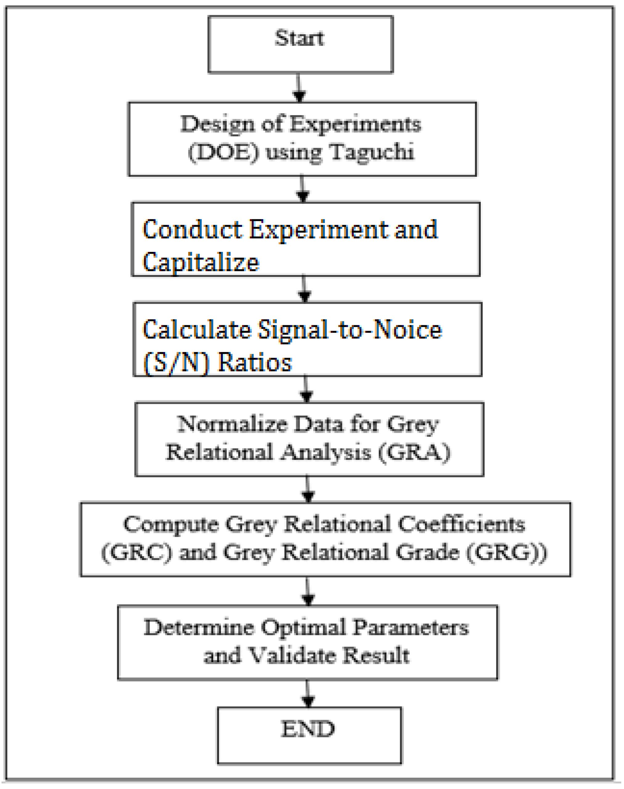
3. Optimization Methodology

Optimization Steps Using Grey Relational Analysis

Step 1: Use the following formula to determine the S/N ratio for the matching replies.

The larger the better.

$${\displaystyle \frac{S}{N}}ratio\left(\eta \right)=-10{log}_{10}\left({\displaystyle \frac{1}{n}}\right)\sum _{i=1}^n{\displaystyle \frac{1}{y_{ij}^2}}$$

(1)

where n = the No. of replications, $y_{ij}$ = observed response value where i = 1, 2, …, n, and j = 1, 2, …, k.

When maximizing the desired quality characteristic is the aim, this is employed tosolve difficulties. The larger-the-better kind is the name given to this dilemma.

The smaller the better.

$${\displaystyle \frac{S}{N}}ratio\left(\eta \right)=-10{log}_{10}\left({\displaystyle \frac{1}{n}}\right)\sum _{i=1}^n{y}_{ij}^2$$

(2)

This problem, where the characteristic is meant to be minimized, is known as the smaller-the-better kind.

The nominal the best.

$${\displaystyle \frac{S}{N}}ratio\left(\eta \right)=10{log}_{10}\left({\displaystyle \frac{{\mu }^2}{{\sigma }^2}}\right)$$

(3)

where

$$\mu ={\displaystyle \frac{y_1+y_2+y_3+y_4\dots \dots +y_n}{n}}$$

$${\sigma }^2={\displaystyle \frac{{\sum {(y}_i-\overline{y})}^2}{n-1}}$$

The purpose of this type of problem, called nominal-the-best is to minimize the mean squared error around a specific goal number. The scenario is reduced to a limited optimization problem in any attempt to achieve the mean on target. Normalization is a procedure that transforms a single data input by scaling it into a range appropriate for further analysis and distributing it uniformly.

Step 2: $y_{ij}$ is normalized as $Z_{ij}$ (0 ≤ $Z_{ij}$ ≤ 1) using a standard formula to eliminate unit differences and reduce variability [21]. Normalization adjusts the data to approximate a value of 1, which can influence ranking. To ensure reliable results, we recommend using S/N ratio values for normalization in Grey Relation Analysis for the S/N ratio with the larger-the-better and using Equation (4) [12].

$$Z_{ij}={\displaystyle \frac{y_{ij}-\mathrm{m}\mathrm{i}\mathrm{n}(y_{ij},i=\mathrm{1,2},\dots n)}{\max \left(y_{ij},i=\mathrm{1,2},\dots n\right)-\mathrm{m}\mathrm{i}\mathrm{n}(y_{ij},i=\mathrm{1,2},\dots n)}}$$

(4)

For an S/N ratio with smaller the better, use Equation (5)

$$Z_{ij}={\displaystyle \frac{\max (y_{ij},i=\mathrm{1,2},\dots n){-y}_{ij}}{\max \left(y_{ij},i=\mathrm{1,2},\dots n\right)-\min (y_{ij},i=\mathrm{1,2},\dots n)}}$$

(5)

For an S/N ratio with nominal-the-best, use Equation (6)

$$Z_{ij}={\displaystyle \frac{{(y}_{ij}-\mathrm{Target})-\mathrm{m}\mathrm{i}\mathrm{n}(\left|y_{ij}-\mathrm{Target}\right|,i=\mathrm{1,2},\dots n)}{\max \left(\left|y_{ij}-\mathrm{T}\mathrm{a}\mathrm{r}\mathrm{g}\mathrm{e}\mathrm{t}\right|,i=\mathrm{1,2},\dots n\right)-\min \left(\left|y_{ij}-\mathrm{Target}\right|,i=\mathrm{1,2},\dots n\right)}}$$

(6)

Step 3: Calculate the grey relational co-efficient for the normalized S/N ratio values

$$\gamma (y_0\left(k\right),y_i\left(k\right))={\displaystyle \frac{{∆}_{\min }+\xi {∆}_{\max }}{{∆}_{0j}\left(k\right)+\xi {∆}_{\max }}}$$

(7)

where

1. j = 1, 2, …, n, k = 1, 2, …, m, n is the No. of experimental data items, and m is the No. of responses.

2. $y_0\left(k\right)$ is the reference sequence $y_0\left(k\right)$ = 1, (k = 1, 2, …, m); $y_j\left(k\right)$ is the specific comparison sequence.

3. ${∆}_{0j}\left(k\right)=‖y_0\left(k\right)-y_j\left(k\right)‖=$ the absolute value of the difference between $y_0\left(k\right) \mathrm{a}\mathrm{n}\mathrm{d} y_j\left(k\right)$.

4. ${∆}_{\min }=\min min‖y_0\left(k\right)-y_j\left(k\right)‖=\mathrm{i}\mathrm{s} \mathrm{t}\mathrm{h}\mathrm{e} \mathrm{s}\mathrm{m}\mathrm{a}\mathrm{l}\mathrm{l}\mathrm{e}\mathrm{s}\mathrm{t} \mathrm{v}\mathrm{a}\mathrm{l}\mathrm{u}\mathrm{e} \mathrm{o}\mathrm{f}{ y}_j\left(k\right)$.

5. ${∆}_{\max }=\max max‖y_0\left(k\right)-y_j\left(k\right)‖=\mathrm{i}\mathrm{s} \mathrm{t}\mathrm{h}\mathrm{e} \mathrm{l}\mathrm{a}\mathrm{r}\mathrm{g}\mathrm{e}\mathrm{s}\mathrm{t} \mathrm{v}\mathrm{a}\mathrm{l}\mathrm{u}\mathrm{e} \mathrm{o}\mathrm{f} y_j\left(k\right)$.

6. $\xi$ is the distinguishing coefficient, defined range 0 ≤ $\xi$ ≤1.

Step 4: Generate the grey relational grade.

$${\overline{\gamma }}_j={\displaystyle \frac{1}{k}}\sum _{I=1}^m\left({\gamma }_{ij}\right)$$

(8)

where k is the No. of performance characteristics, and ${\overline{\gamma }}_j$ is the grey relational grade for the jth experiment.

Step 5: Determine the best combination of factors and levels based on the grey relational grade; a higher grade denotes a higher-quality result. This makes it possible to choose the ideal levels for controllable elements and estimate the effects of components.

For instance, we compute the average of grade values (AGV) for each level j, represented as [${AGV}_{ij}$], in order to assess the influence of factor i. The effect, E_i, is then defined as follows:

$${\mathrm{E}}_i=\max \left({AGV}_{ij}\right)-\min \left({AGV}_{ij}\right)$$

(9)

The optimal level j* is established if the factor i is adjustable by

$$j^{\mathrm{*}}={\max }_j\left({AGV}_{ij}\right)$$

(10)

Step 6: Perform ANOVA to identify significant factors by analyzing the impact of individual process parameters. While the Taguchi Method cannot isolate the effect of specific parameters, ANOVA compensates by calculating the percentage contribution of each factor to the total variation (SST) [21,22,23]. The SST is divided into the sum of squared deviations caused by the process parameters and the error. A factor’s significance is determined by its F-value, with larger F-values indicating a greater effect on performance characteristics.

Step 7: Determine the predicted optimum condition by calculating the estimated S/N ratio using the optimal design parameter levels. This is performed based on the factor levels derived from Equations (9) and (10) to verify the quality characteristic.

$$\widehat{\eta }={\eta }_m+{\displaystyle \frac{1}{k}}\sum _{I=1}^q\left({\overline{\eta }}_i-{\eta }_m\right)$$

(11)

${\eta }_m$ = Average SN ratio.

$\overline{\eta }$ = Average SN ratio corresponding to ith significant factor on jth level.

q = Number of significant factors.

4. Implementation of Methodology

Step 1: Use one of the equations to find the S/N ratios for a certain reaction and the expected S/N ratios of the initial conditions, depending on the kind of quality attributes, (1), (2), or (3). Table 4 displays the calculated S/N ratios for each quality attribute.

Step 2: Normalize the S/N ratio values using Formulas (4)–(6).

Table 5. S/N ratio and normalization data.

Trial	S/N Ratio					Normalization Data
	NOx (ppm)	HC (ppm)	SMOKE (% Vol)	SFC (g/kWh)	BTE (%)	NOx (ppm)	HC (ppm)	SMOKE (% Vol)	SFC (g/kWh)	BTE (%)
1	−45.5	−24.6	4.437	4.44	23.1	0.915	0.673	1.000	0.033	0.008
2	−58.6	−28.3	−12.26	7.33	25.9	0.345	0.490	0.888	0.600	0.425
3	−49	−23.5	−23.29	8.64	27.2	0.837	0.714	0.551	0.800	0.665
4	−49	−28	−27.49	10.2	28.7	0.836	0.510	0.260	1.000	1.000
5	−39.1	−18.1	0.9151	4.88	23.5	1.000	0.857	0.990	0.133	0.068
6	−45.6	−21.6	−14.32	6.38	25	0.914	0.776	0.853	0.433	0.285
7	−62	−28.3	−18.89	9.37	27.9	0.000	0.490	0.737	0.900	0.817
8	−60.6	−34	−25.11	9.12	27.8	0.163	0.000	0.442	0.867	0.790
9	−52.8	−25.6	−9.827	4.29	23	0.705	0.633	0.920	0.000	0.000
10	−59	−29.2	−18.17	8.18	26.8	0.313	0.429	0.760	0.733	0.593
11	−49.4	−24.1	−17.03	9.37	28	0.826	0.694	0.792	0.900	0.826
12	−48.5	−30.1	−23.92	10.2	28.7	0.850	0.367	0.516	1.000	0.998
13	−46.9	0	1.9382	4.88	23.5	0.888	1.000	0.994	0.133	0.067
14	−49.2	−9.54	−8.627	6.38	25	0.831	0.959	0.933	0.433	0.282
15	−60.7	−29.2	−22.98	9.37	28	0.156	0.429	0.567	0.900	0.840
16	−60	−33.8	−30.05	9.12	27.8	0.226	0.020	0.000	0.867	0.791

presents the findings.

Step 3: Perform the analysis of grey relations. Equation (7) can be used to obtain the grey relationship coefficient for the normalized S/N ratio values based on the data in Table 4. Because all process parameters are equally weighted, Equation (7)’s value for ξ is 0.5 [12]. Table 5 and

Table 6. Grey relation deviation, coefficient, grade, and rank.

Grey Relation Deviation					Grey Relation Coeff					Grade	Rank
NOx	HC	SMOKE	SFC	BTE	NOx	HC	SMOKE	SFC	BTE
0.085	0.327	0.000	0.967	0.992	0.855	0.605	1.000	0.341	0.335	0.627	9
0.655	0.510	0.112	0.400	0.575	0.433	0.495	0.817	0.556	0.465	0.553	13
0.163	0.286	0.449	0.200	0.335	0.754	0.636	0.527	0.714	0.599	0.646	7
0.164	0.490	0.740	0.000	0.000	0.753	0.505	0.403	1.000	1.000	0.732	2
0.000	0.143	0.010	0.867	0.932	1.000	0.778	0.981	0.366	0.349	0.695	5
0.086	0.224	0.147	0.567	0.715	0.853	0.690	0.772	0.469	0.412	0.639	8
1.000	0.510	0.263	0.100	0.183	0.333	0.495	0.655	0.833	0.732	0.610	10
0.837	1.000	0.558	0.133	0.210	0.374	0.333	0.473	0.789	0.704	0.535	15
0.295	0.367	0.080	1.000	1.000	0.629	0.576	0.862	0.333	0.333	0.547	14
0.687	0.571	0.240	0.267	0.407	0.421	0.467	0.675	0.652	0.551	0.553	12
0.174	0.306	0.208	0.100	0.174	0.741	0.620	0.706	0.833	0.742	0.729	3
0.150	0.633	0.484	0.000	0.002	0.769	0.441	0.508	1.000	0.997	0.743	1
0.112	0.000	0.006	0.867	0.933	0.817	1.000	0.987	0.366	0.349	0.704	4
0.169	0.041	0.067	0.567	0.718	0.747	0.925	0.881	0.469	0.410	0.686	6
0.844	0.571	0.433	0.100	0.160	0.372	0.467	0.536	0.833	0.757	0.593	11
0.774	0.980	1.000	0.133	0.209	0.393	0.338	0.333	0.789	0.705	0.512	16

presents the findings.

Step 4: Equation (8) can then be used to calculate the grey relational grade. Lastly, the grades are taken into account while optimizing the design issue with multiple response parameters. Table 6 presents the findings.

Step 5: Using Equation (9), the primary impacts and the factor effects based on the grey relational grade value are listed in Table 6.

Regression Equation

GRADE = 0.6315 + 0.0082 BLEND_DISEL − 0.0119 BLEND_G1B10 + 0.0114 BLEND_G2B10 − 0.0077
BLEND_G3B10 + 0.0117 LOAD_25% − 0.0235 LOAD_50% + 0.0129 LOAD_75% − 0.0011 LOAD_100% +
0.0048 CR_17 − 0.0048 CR_18 − 0.0653 EGR_0% + 0.0653 EGR_10%

Step 6: The ideal parameter circumstances are G2B10, 100% load, CR17, and 10% EGR while taking into account the maximizing of grade values Table 6.

Table 7. Model Summary.

S	R-sq	R-sq(adj)	PRESS	R-sq(pred)	AICc	BIC
0.047949	82.05%	61.53%	0.08408	6.21%	−1.02	−37.3

shows model summary, which shows model is perfect and valid.

Step 7: ANOVA is created to determine the important elements using the grey grade value.

Table 8. Response table for means (main effects).

Level	BLEND	LOAD	CR	EGR
1	0.6397	0.6432	0.6363	0.5662
2	0.6196	0.608	0.6267	0.6968
3	0.6429	0.6444
4	0.6238	0.6304
Delta	0.0233	0.0364	0.0097	0.1305
Rank	3	2	4	1

displays the response table for means, which highlights crucial information about the response variable across different factors and aids in the interpretation of ANOVA by displaying trends and identifying the most relevant factors influencing the result.

ANOVA findings are displayed in

Table 9. Analysis of variance.

Source	DF	Seq SS	Contribution	Adj SS	Adj MS	F-Value	p-Value
BLEND	3	0.001596	1.78%	0.001596	0.000532	0.23	0.872
LOAD	3	0.003424	3.82%	0.003424	0.001141	0.5	0.696
CR	1	0.000375	0.42%	0.000375	0.000375	0.16	0.698
EGR	2	0.068156	76.03%	0.068156	0.068156	29.65	0.001
Error	7	0.016093	17.95%	0.016093	0.002299
Total	15	0.089644	100.00%

. According to ANOVA, the EGR (76.03%) has the greatest impact on engine emissions and performance, followed by load (3.82%), blend (1.78%), and the CR (0.42%).

Step 8: The following model is used to determine the predicted mean at the optimal settings (μ), which is used to estimate the optimum condition.

$$\mathsf{\mu }=\overline{\mathrm{G}2\mathrm{B}10}+\overline{\mathrm{L}\mathrm{o}\mathrm{a}\mathrm{d}}+\overline{CR}+\overline{EGR}-2\ast {\overline{T}}_{gg}$$

(12)

where ${\overline{T}}_{gg}$ is the average grey grade mean, and $\overline{\mathrm{G}2\mathrm{B}10}$, $\overline{\mathrm{L}\mathrm{o}\mathrm{a}\mathrm{d}}$, $\overline{CR}$, $\overline{EGR}$ are the mean values of the grey relational grade with the parameters at optimal levels. At ideal conditions, the predicted mean (μ) is 0.7430564232399214.

The confidence interval (CI) is calculated as

$$\mathrm{C}.\mathrm{I}.=\sqrt{F_{\alpha }\left(1, f_e\right)V_e\left[{\displaystyle \frac{1}{{\eta }_{eff}}}+{\displaystyle \frac{1}{R}}\right]}$$

(13)

where R is the number of confirmation tests, ${\eta }_{eff}$ is the effective total number of tests, $V_e$ is the error mean square, $f_e$ is the error degrees of freedom, and α is the risk. The F ratio at a significance level of α% is denoted by F_α(1, $f_e$).

$${\eta }_{eff}={\displaystyle \frac{Total number of observations}{1+\left(Total degress of free domassociated with it mesused in estimating \mu Ra\right)}}$$

(14)

The 95% confidence interval of the expected optimum condition is thus provided by the following model, where ${\mathsf{\mu }}_{cgg}$ = the grey relational grade value following the execution of the confirmation trials with optimal configuration points, i.e., G2B10, 100% load, CR17, 10% EGR.

Taguchi analysis NOx vs. factors are shown in Figure 4. NOx increases with load due to increases in temperature. As the CR ratio increases, NOx also increases again, reason being the increase in temperature inside the combustion chamber. For G2B10, NOx is less as compared to the other blend of G1B10 and G3B10, due to higher density, less calorific value, and the EGR system. Figure 5 shows the HC versus the BLEND, LOAD, CR, and EGR. For G3B10, the HC emission is significantly less as compared to the remaining blend due to proper combustion and less viscosity [18].

The HC increases with load. CR and EGR reduces the HC emission due to enhanced combustion and Net Heat Release rate improvement. Figure 6 shows smoke opacity emission vs. input factors. G1B10 and 10% EGR have a less amount of smoke opacity emissions. Due to the recirculation of exhaust gases, smoke opacity reduces. Figure 7 shows the SFC vs. input factors. The SFC for G2B10 is less due to less density of neem oil. The SFC decreases with the increase in load as the BP increases with load. There is notas much effect of the CR and EGR on the SFC.

Figure 8 shows BTE vs. input factors. G2B10 blend impressed more as compared to another blend due to higher density and higher cetane number. There is less effect of the CR and EGR on BTE. Figure 9 depicts the effects of factors on grade values, demonstrating that the optimal parameter configuration is G2B10, 75% load, 17CR, and 10% EGR. Figure 10 shows probability, fits, histograms, and order plots for the grey relation grade. The residual plots indicate that the assumptions of the regression model (normality of residuals, constant variance, and independence) are generally met. This suggests that the model is a good fit for the data and does not exhibit significant biases or inconsistencies.

The optimal solution using Grey Relation Analysis is G2B10, 100% load, 17CR, 10%EGR, and corresponding response values and optimal parameter conditions using Anova are G2B10,75% Load, 17CR, 10%EGR and optimum response, as shown in

Table 10. Optimal solution and optimum parameter setting.

Optimization	Blend	Load	CR	EGR	NOx (ppm)	HC (ppm)	SMOKE (% Vol)	SFC (g/kWh)	BTE (%)
GRA	G2B10	100%	17	10%	266	18	15.7	0.31	27.27
Optimal parameter setting	G2B10	75%	17	10%	294	16	7.1	0.34	25

.

5. Confirmation Experiment

A confirmation experiment was performed at the optimal settings to validate improvements in CRDI CI engine performance and emission reduction. The results, shown in Table 10, yielded a grey relational grade (${\mathsf{\mu }}_{cgg}$) of 0.7119876663008827, within the 95% confidence interval of the predicted optimum. This value represents a negative 3.14% improvement over the predicted mean. As a result, the GRA results are retained as the ideal parameter setting. The Taguchi approach in conjunction with the Grey Relational Analysis was successful in optimizing multi-response problems, such as NOx, HC, smoke, SFC, and BTE. The optimal blend, G2B10 (10% cottonseed oil, 80% neem oil, 10% orange peel oil), achieved enhanced ignition with a shorter delay and higher peak pressure, NOx reduced by 10%, Brake thermal efficiency improved by 9.08%. The HC emission decreased by 10%. The average smoke opacity decreased by 27.65%. Cylinder pressure remains unchanged, but the Net Heat Release rate improved by 2%.

6. Conclusions

Tests were carried out using Biodiesel and its blend. Output parameters such as emissions like NOx, HC and smoke and performance parameters like SFC and BTE were measured for different input parameters such as blend%, load, CR and EGR. The following conclusions can be drawn:

• Grey Relational Analysis is a highly helpful tool for estimating the NOx, HC, smoke, SFC, and BTE with many objectives in the Taguchi approach for optimizing the multi-response issues.
• Because it does not require complex mathematical theory or calculation, engineers without solid experience in statistics can use it.
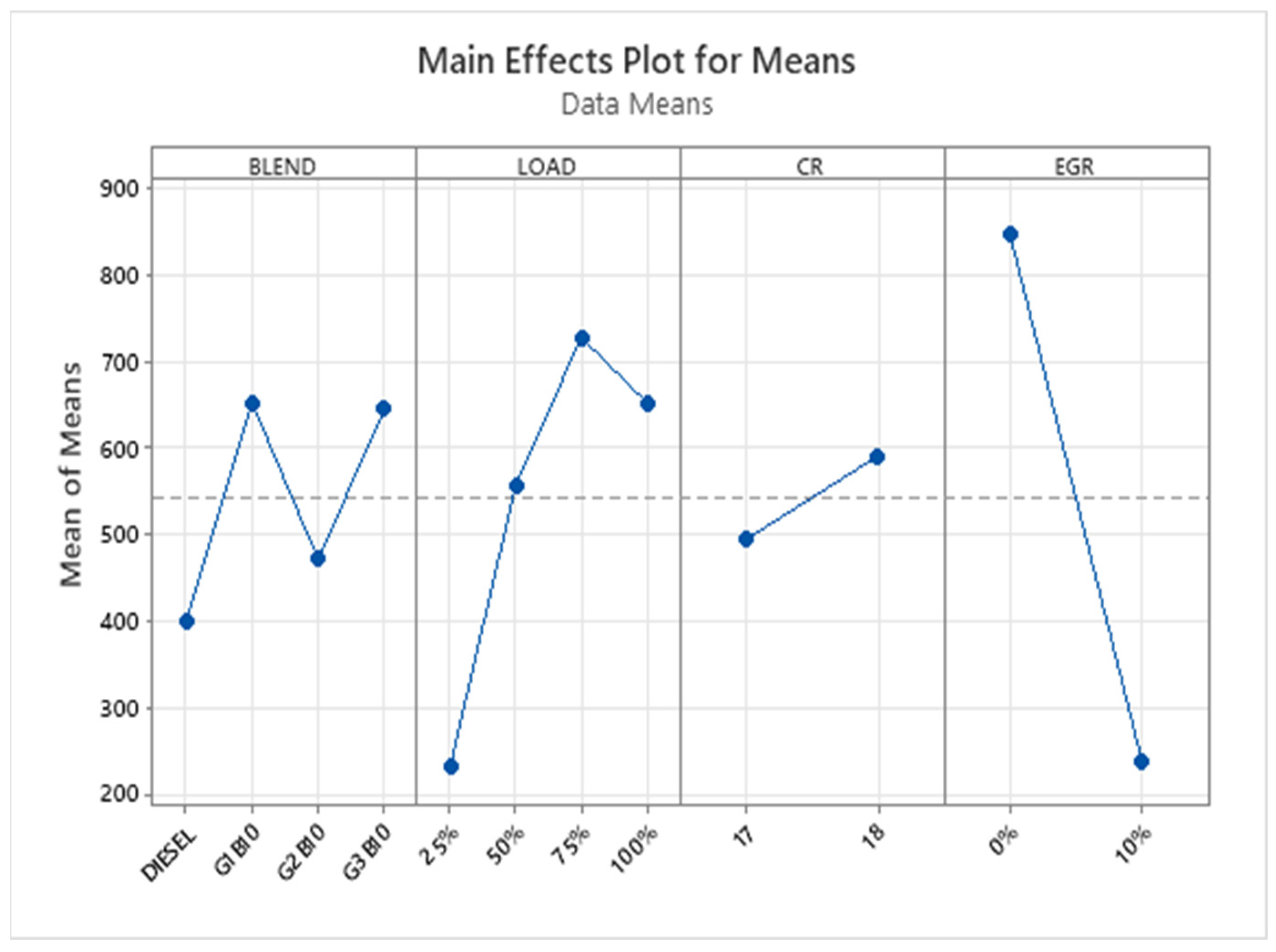
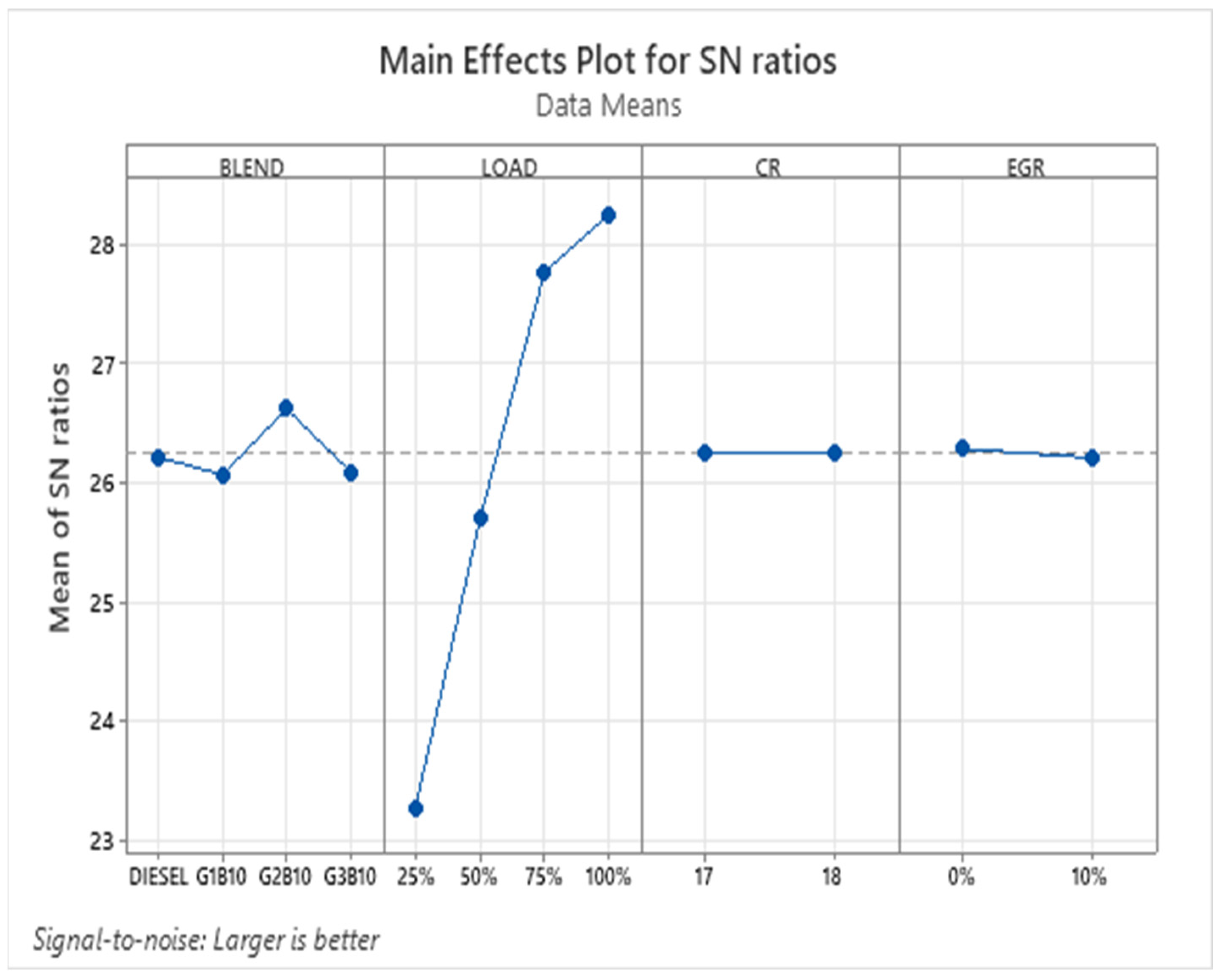
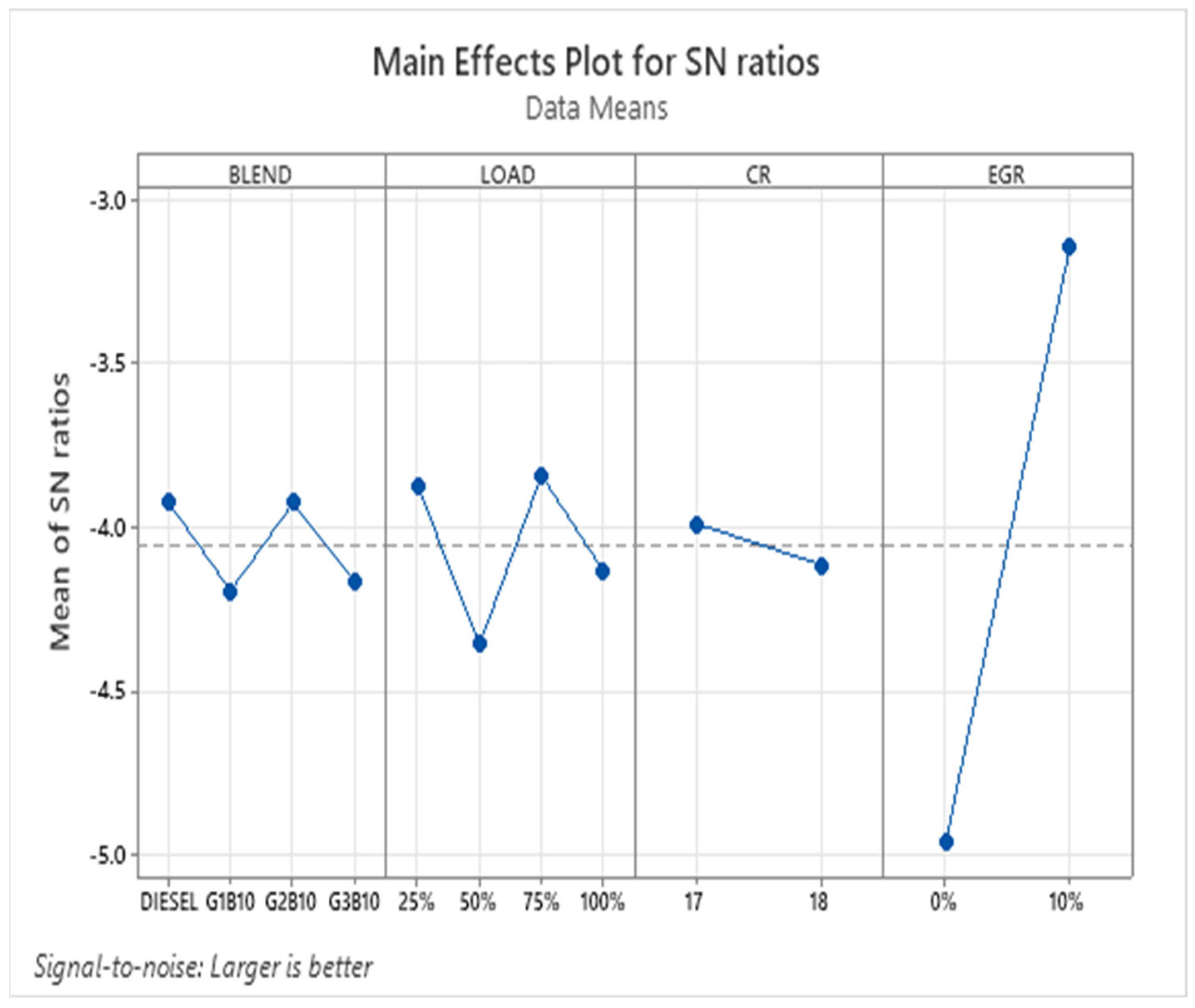
• Load (62.53%) influences more on engine performance and emissions followed by the EGR (33.92%), blend (0.59%) and CR (0.02%).
• Optimum parameter settings from GRA and ANOVA is found to be G2B10, 100%Load, 17CR, 10%EGR and optimum values of NOx = 266 ppm, HC = 18 ppm, smoke = 15.7% Vol, SFC = 0.31 g/kWh, and BTE = 27.27%.

This study successfully demonstrates the feasibility of a ternary blend of cottonseed oil, neem oil, and orange peel oil as an alternative fuel for diesel engines. The optimized blend achieved significant improvements in combustion and performance while reducing exhaust emissions. The use of advanced optimization tools like Grey Relation Analysis with Taguchi ensured the precise identification of the optimal blend ratio, paving the way for large-scale implementation. The ternary blend outperformed binary blends and individual oils in terms of both performance and emissions, highlighting the synergistic effects of the selected oils.

References

1. Knothe, G.; Razon, L.F. Biodiesel fuels. Prog. Energy Combust. Sci. 2017, 58, 36–59. [Google Scholar] [CrossRef]
2. Ramadhas, A.S.; Jayaraj, S.; Muraleedharan, C. Use of vegetable oils as I.C. engine fuels—A review. Renew. Energy 2004, 29, 727–742. [Google Scholar] [CrossRef]
3. Kalam, M.A.; Masjuki, H.H. Biodiesel from palmoil—An analysis of its properties and potential. Biomass Bioenergy 2002, 23, 471–479. [Google Scholar] [CrossRef]
4. Çiftçi, B.; Karagöz, M.; Aydin, M.; Çelik, M.B. The effect of fusel oil and waste biodiesel fuel blends on a CI engine performance, emissions, and combustion characteristics. J. Therm. Anal. Calorim. 2024, 149, 7783–7796. [Google Scholar] [CrossRef]
5. Chauhan, B.S.; Kumar, N.; Jun, Y.D.; Lee, K.B. Performance and emission study of preheated Jatropha oil on medium capacity diesel engine. Energy 2010, 35, 2484–2492. [Google Scholar] [CrossRef]
6. Jain, S.; Sharma, M.P. Prospects of biodiesel from Jatropha in India: A review. Renew. Sustain. Energy Rev. 2010, 14, 763–771. [Google Scholar] [CrossRef]
7. Bhale, P.V.; Deshpande, N.V.; Thombre, S.B. Improving the low temperature properties of biodiesel fuel. Renew. Energy 2009, 34, 794–800. [Google Scholar] [CrossRef]
8. Ramachandra, R.; Pandurangadu, V.; Raju KA, K. Comparison and Evaluation of Performance and Emission Characteristics of Four Stroke Diesel Engine with Neem and Cotton Seed Bio Diesels. Int. J. Eng. Technol. Res. 2014, 2, 282–285. [Google Scholar]
9. Dhamodaran, G.; Krishnan, R.; Pochareddy, Y.K.; Pyarelal, H.M.; Sivasubramanian, H.; Ganeshram, A.K. A comparative study of combustion, emission, and performance characteristics of rice-bran-, neem-, and cottonseed-oil biodiesels with varying degree of unsaturation. Fuel 2017, 187, 296–305. [Google Scholar] [CrossRef]
10. Gad, M.S.; El-Shafay, A.S.; Alqsair, U.F.; Ağbulut, Ü.; Attia, E.A. Multi-objective optimization based grey relational analysis and investigation of using the waste animal fat biodiesel on the engine characteristics. Fuel 2023, 343, 127950. [Google Scholar] [CrossRef]
11. Karnwal, A.; Hasan, M.M.; Kumar, N.; Siddiquee, A.N.; Khan, Z.A. Multi-response optimization of diesel engine performance parameters using thumba biodiesel-diesel blends by applying the Taguchi method and grey relational analysis. Int. J. Automot. Technol. 2011, 12, 599–610. [Google Scholar] [CrossRef]
12. Muqeem, M.; Sherwani, A.F.; Ahmad, M.; Khan, Z.A. Taguchi based grey relational analysis for multi response optimisation of diesel engine performance and emission parameters. Int. J. Heavy Veh. Syst. 2020, 27, 441–460. [Google Scholar] [CrossRef]
13. Asokan, M.A.; Prabu, S.S.; Prathiba, S.; Sukhadia, D.S.; Jain, V.; Sarwate, S.M. Emission and performance behavior of Orange peel oil/diesel blends in di diesel engine. Mater. Today Proc. 2021, 46, 8114–8118. [Google Scholar] [CrossRef]
14. Indian Council of Agricultural Research. Annual Report 2023–2024. 2016, pp. 1–23. Available online: https://icar.org.in/sites/default/files/2024-09/ICAREngAR_2023-24forweb.pdf (accessed on 1 September 2024).
15. Gopidesi, R.K.; Reddy, V.R.K.; Kumar, V.S.S.; Vardhan, T.V.; Reddy, V.J. Effect of cotton seed oil in diesel engine performance emission and combustion characteristics. Int. J. Innov. Technol. Explor. Eng. 2019, 8, 2602–2605. [Google Scholar]
16. Ranjith, V.V.; Thanikaikarasan, S. Prediction of Exhaust Gas Emission characteristics using Neem oil blended bio-diesel in diesel engine. Mater. Today Proc. 2020, 21, 870–875. [Google Scholar] [CrossRef]
17. Ashok, B.; Nanthagopal, K.; Perumal, D.A.; Babu, J.M.; Tiwari, A.; Sharma, A. An investigation on CRDi engine characteristic using renewable orange-peel oil. Energy Convers. Manag. 2018, 180, 1026–1038. [Google Scholar] [CrossRef]
18. Mourshed, M.; Ghosh, S.K.; Islam, M.W. Experimental investigation of cotton (Gossypium hirsutum) seed oil and neem (Azadirachta indica) seed oil methyl esters as biodiesel on DI (Direct Injection) engine. Int. J. Ambient Energy 2022, 43, 1772–1782. [Google Scholar] [CrossRef]
19. Rastogi, A.; Shaban, M.; Saxena, S.; Singh, T.P. Neem Biodiesel: An Alternative Fuel. Innovare J. Eng. Technol. 2021, 9, 18–21. [Google Scholar] [CrossRef]
20. Mishra, D.; Kumar, N.; Chaudhary, R. Effect of orange peel oil on the performance and emission characteristics of diesel engine fueled with quaternary blends. Energy Sources Part A Recovery Util. Environ. Eff. 2022, 45, 650–660. [Google Scholar] [CrossRef]
21. Abifarin, J.; Ofodu, J. Modeling and Grey Relational Multi-response Optimization of Chemical Additives and Engine Parameters on Performance Efficiency of Diesel Engine. Int. J. Grey Syst. 2022, 2, 16–26. [Google Scholar] [CrossRef]
22. Gul, M.; Shah, A.N.; Jamal, Y.; Masood, I. Multi-variable optimization of diesel engine fuelled with biodiesel using grey-Taguchi method. J. Braz. Soc. Mech. Sci. Eng. 2016, 38, 621–632. [Google Scholar] [CrossRef]
23. Brijesh, P.; Chowdhury, A.; Sreedhara, S. The simultaneous reduction of NO x and PM using ultra-cooled EGR and retarded injection timing in a diesel engine. Int. J. Green Energy 2015, 12, 347–358. [Google Scholar] [CrossRef]
Figure 1. Testing fuels.
Fire 08 00083 g001
Figure 2. Experimental setup.
Fire 08 00083 g002
Figure 3. Flowchart for illustrating the optimization process.
Fire 08 00083 g003
Figure 4. Taguchi analysis: NOx vs. BLEND, LOAD, CR, and EGR.
Fire 08 00083 g004
Figure 5. Taguchi analysis: HC vs. BLEND, LOAD, CR, and EGR.
Fire 08 00083 g005
Figure 6. Taguchi analysis: SMOKE vs. BLEND, LOAD, CR, and EGR.
Fire 08 00083 g006
Figure 7. Taguchi Analysis: SFC vs. BLEND, LOAD, CR, and EGR.
Fire 08 00083 g007
Figure 8. Taguchi Analysis: BTE vs. BLEND, LOAD, CR, and EGR.
Fire 08 00083 g008
Figure 9. Factor effects on grade values.
Fire 08 00083 g009
Figure 10. Probability fits, histograms, and order plots.
Fire 08 00083 g010