Abstract
This study investigates the physical interactions and between forest fires and the atmosphere, which often lead to conditions favourable to instability and the formation of pyrocumulus (PyCu). Using the coupled atmosphere–fire spread modelling framework, WRF-SFIRE, the Portuguese October 2017 Quiaios wildfire, in association with tropical cyclone Ophelia, was simulated. Fire spread was imposed via burnt area data, and the fire’s influence on the vertical and surface atmosphere was analysed. Simulated local atmospheric conditions were influenced by warm and dry air advection near the surface, and moist air in mid to high levels, displaying an inverted “V” profile in thermodynamic diagrams. These conditions created a near-neutrally unstable atmospheric layer in the first 3000 m, associated with a low-level jet above 1000 m. Results showed that vertical wind shear tilted the plume, resulting in an intermittent, high-based, shallow pyroconvection, in a zero convective available potential energy environment (CAPE). Lifted parcels from the fire lost their buoyancy shortly after condensation, and the presence of PyCu was governed by the energy output from the fire and its updrafts. Clouds formed above the lifted condensation level (LCL) as moisture fluxes from the surface and released from combustion were lifted along the fire plume. Clouds were primarily composed of liquid water (1 g/kg) with smaller traces of ice, graupel, and snow (up to 0.15 g/kg). The representation of pyroconvective dynamics via coupled models is the cornerstone of understanding the phenomena and field applications as the computation capability increases and provides firefighters with real time extreme fire conditions or predicting ahead of time.
1. Introduction
Wildfires have significant negative impacts on the ecology and socioeconomic activities of the affected populations. Fire–atmosphere interactions promote fire risk, with atmospheric instability and pyroconvection as their drivers. Pyroconvective clouds can be classified as pyro cumulus (PyCu) [1] or pyrocumulonimbus (PyCb), the latter being defined as clouds generated by buoyant energy imparted to the atmosphere by surface heating from fire [2].
Research into proconvective events has been carried out, especially in the recent decades, to better understand the processes that contribute to the generation of pyroconvective clouds. Potter (2012) [3] reviewed the scientific literature, including the vertical and surface analyses of the atmosphere, wind speed, humidity, and the processes occurring in the boundary layer, highlighting the nonlinear nature of fire–atmosphere interactions. Climate change has been a driver of changes, amplifying the frequency and intensity of fire-prone weather, affecting ecosystem dynamics, and improving fuel availability [4,5,6,7].
It is difficult to predict the dynamics that lead to the formation and development of pyrocovenction. Several studies have attempted to establish a link between the effect of fuel combustion and latent heat release into the atmosphere, and buoyancy production from fire-modified Convective Available Potential Energy (CAPE) via increments in mixing ratio and temperature when generating pyroconvection [8,9,10]. While naturally occurring instability is associated with the presence of CAPE, several PyCb-producing wildfires have been found to occur under low or non-existent environmental CAPE values [11], often in fires on the leading edge of a disturbance [12,13,14]. PyCb producing fires frequently occurred in high LCL, above 5 km, under an “inverted V” profiled atmosphere, dry and hot base, and moist mid to high levels, providing wildfire favourable conditions at the surface and downburst potential from evaporative cooling downdrafts [15,16,17]. Tory studied the thermodynamics of a wildfire plume to try and predict the formation of pyroconvection, attributing a firepower threshold produced by the surface fire that would result in PyCb initiation, adding the effect of wind, dilution and tilting plumes to buoyancy [9,18].
Coupled fire–atmosphere models, with or without chemistry, have often been used to represent wildfire thermodynamics and the development of pyroconvective cloud formation. Reference [19] described several coupled models (that is, WRF-SFIRE, MESO-NH, WFDS, etc.), from micro to mesoscale, that aim to reproduce feedback between the fire fluxes and the atmosphere. Others, such as ACCESS-Fire, have been used more recently to understand how fire behaviour increases the fire spread rate and spotting during extreme fire events in Australia [20]. Previous model simulations using ATHAM, without using a coupled fire spread module, have shown that strong pyroconvection can also lift smoke aerosols to the lower stratosphere, reproducing updrafts and the entrainment effect of the rising plume, using surface fire observation emissions as input [13,21]. The WRF-SFIRE model has been used in several studies, including the effect of PBL circulation on fire plumes amplification [20] and the impact of wildfire–atmosphere dynamics’ on smoke and particle dispersion [22].
The Mediterranean basin is one of the main hotspots for forest fire occurrence in Europe, with 85% of the total area burnt in Portugal, Spain, France, Italy, and Greece [23]. Traditionally, extreme fire events in Portugal follow a pattern of easterly, dry, and hot winds associated with the Iberian thermal low [24], co-occurring with heat-waves and extended drought periods [25]. In recent decades, climate change has prompted an increase in fire prone weather, namely in the central and northern regions of Portugal where more flammable forested regions are located [26]. The year 2017 was particularly costly on a socio-economic level, with 117 fatalities and EUR 1.5 billion in estimated damages [27]. The unpredictable nature of extreme wildfires has, as recently as 2024, turned a below average burnt area year into a 22% above average due the occurrence of late-season September wildfires, despite having the third lowest total number of registered wildfires since 2014 [28].
The October 2017 wildfires differed in the sense that an approaching disturbance from the west, Tropical Cyclone Ophelia, was responsible for the out-of-season hot and windy weather conditions.
Several studies and reports have analysed pre-fire conditions on fuels to explain the extreme wildfire behaviour. These studies indicate that vegetation stress from prolonged droughts significantly increases the potential and severity of extreme fire events [12,29,30,31]. Inland fires showed that PyCb formation was offset by the arrival of moisture from shifting winds associated with the circulation of tropical cyclones. During the October 2017 extreme fire events, coastal fires produced weaker pyroconvection, consisting of PyCu, and were mainly wind-driven [32].
Coupled atmosphere–fire modelling of wildfires that comprised the extreme fire event of October 2017 has been carried out using the atmosphere–fire coupled model Meso-NH/ForeFire, showing the development of PyCu from fire induced vertical moisture fluxes [33]. A model intercomparison between Meso-NH/ForeFire and WRF-SFIRE showed the latter’s inability to form pyroconvection in similar scenarios [34].
Few wildfire studies using coupled atmosphere–fire models have been carried out, with an emphasis on pyroconvection. The Meso-NH/ForeFire has been successfully employed to simulate triggering pyroconvection in the June 2017 Pedrogão Grande wildfires, using a simplified and uniform fuel model. The aim of the present study is to show that results achieved with WRF-SFIRE can indeed simulate the pyroclouds and explain how the thermodynamics of the fire helped to develop pyroconvection under the effect of Tropical Cyclone Ophelia, using WRF-SFIRE, and provide further insight on the dynamics of the fire plume and cloud formation.
To analyse the dynamics of atmosphere–fire interactions, this study presents a modelled case study of the Quiaios wildfire that occurred in Portugal (west coast of the Iberian Peninsula) in October 2017, using the atmosphere–fire coupled model WRF-SFIRE (Weather Research and Forecast-SFIRE) [35,36,37]. Furthermore, forest fire event reports describe the spread of the Quiaios fire as being governed mainly by the wind and not by the dynamic processes of the fire plume, without any special reference to pyroconvective observations [29,31,38]. However, photographic evidence [39] shows that the pyroconvective activity of these coastal fires developed moderate, low-altitude PyCu (up to 5000 m) [32].
This article is structured in three major sections: Data and Methods, Results and Discussion, and Conclusions.
2. Data and Methods
2.1. The WRF-SFIRE Coupled Atmosphere–Fire Model
WRF-SFIRE couples the Advanced Research Weather (ARW) core from the WRF [37] with a semi-empirical fire-spread SFIRE model. The SFIRE model is a two-dimensional model that uses the level-set method to advance the fireline, which involves moving an implicit surface on a velocity field [40]. Fire spread rates are calculated based on the model described in [41], given the 13 National Forest Fire Laboratory (NFFL) fuel properties described by [42,43].
The SFIRE module allows for the interaction between WRF’s atmospheric grid and SFIRE’s sub-grid in the form of heat and moisture, providing feedback between the two interfaces. The terrain gradient and fuel maps are necessary inputs required by the model before initialisation. Fuels are treated as static fields and provide information used for fire spread. However, fuel moisture can be fed into the model dynamically using the coupled moisture model or provided by a static array [35].
By using WRF-SFIRE, we aim to expand on alternative atmosphere–fire coupled models, providing additional insights on previously performed studies, emphasising the capability of pyroconvective cloud production. Coupling with the widely used WRF atmospheric module provides versatility in a wide range of wildfire–atmosphere coupled studies.
2.2. Model Setup
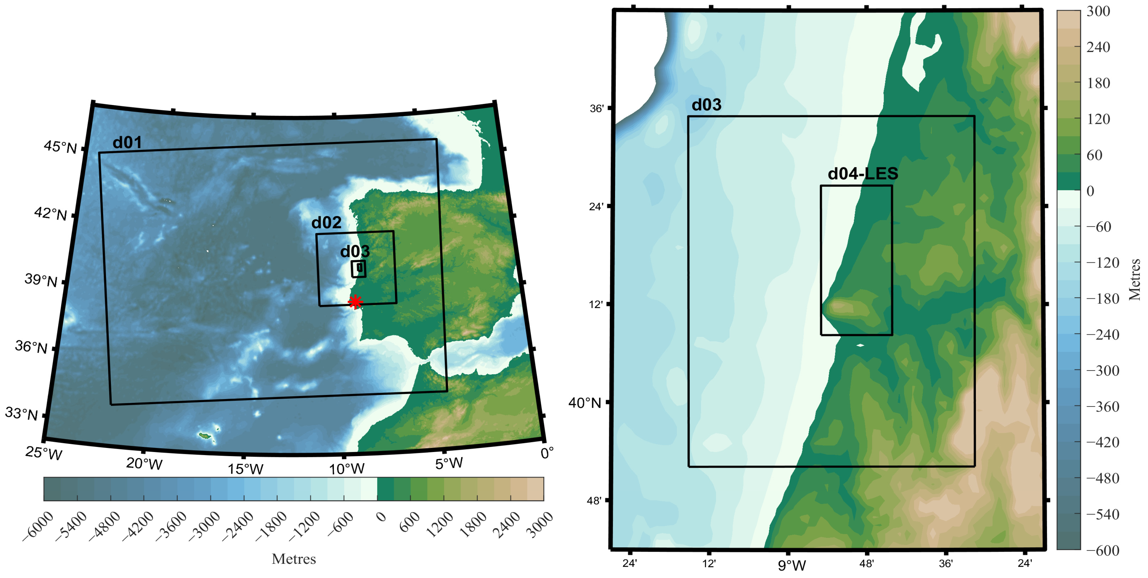
The Quiaios coast wildfire area was primarily composed of a homogenous fuel cover, mostly maritime pine [32], and flat topography. A four-nested domain setup was used, with horizontal grid resolutions of 7.5 km, 2.5 km, 0.5 km, and 0.1 km for domains d01 through d04-LES (Figure 1 and Figure 2) across 51 vertical levels, distributed automatically by WRF. The model time steps used were 22.5 s, 7.5 s, 1.5 s, and 0.3 s, according to the increase in the horizontal resolution.

Figure 1.
Model domain’s configuration, with the location of the vertical sounding used in the model validation represented as a red asterisk. Shading colours show the topographical height.
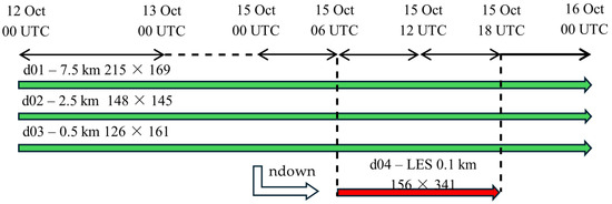
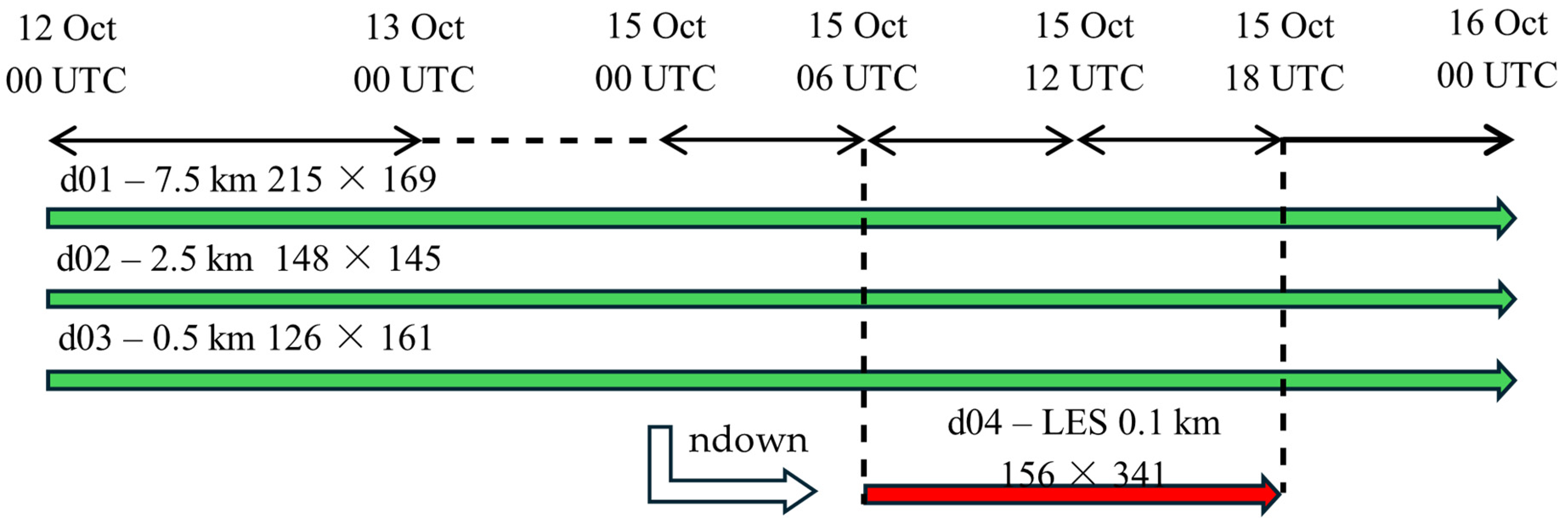
Figure 2.
Schematic illustration of the WRF model simulation approach used during the model runs performed in this study. d04-LES.
The simulations were performed using a two-part process: the main run (domains d01 to d03) was run separately from the d04-LES run. The main run was initialised on 12th of October 2017, at 00:00 UTC, and ended on the 16th of October 2017, at 00:00 UTC. The parent domain d01 was extended westward to capture and simulate the atmospheric processes of the tropical cyclone Ophelia, capturing the zonal flow and large-scale circulation. The d04-LES experiment was run standalone, and was reinitialized using ndown, from the output of the d03 domain between the 15th of October at 06:00 UTC and 18:00 UTC, as illustrated in Figure 2. Two d04-LES runs were performed, with and without fire, henceforth referred to as environmental runs, to evaluate differences in the fire-altered environment. The meteorological initial and boundary conditions were given by the ERA-5 reanalysis from the European Centre for Medium-Range Weather Forecasts (ECMWF) [44]. Additionally, during the model run, grid analysis nudging was applied to the temperature, water vapour, and wind fields every 6 h to the domain d01.
The physical parameterisations chosen for these simulations are summarised in Table 1. Briefly, the WRF Single momentum Microphysics with 6 hydrometeor species was used for the microphysics option [45]; the cumulus parametrisations were set to the Kain–Fritsch scheme [46] only for d01, explicitly resolving them in the subsequent finer grid scales; the Longwave and Shortwave radiation were parametrised by the Rapid Radiative Transfer Model [47]; the Yonsei University’s Planetary Boundary Layer (PBL) non-local scheme was used for parametrising the PBL in d01–d03 [48], and turned off for d04-LES for the Large Eddy Simulation run; and the Noah-Multiparameter was used as a Land Surface Model [49,50].

Table 1.
Model physical parametrisation options used in this study. Model switch options are denoted in parentheses.
The use of high-resolution topography and up-to-date landuse have been shown to achieve a better performance in simulating temperature and wind speed [51,52,53]. Hence, the high-resolution topographical data from the Shuttle Radar Topography Mission (SRTM, ~90 m) was used for the atmospheric simulations [54] and the Corine Land Cover 2012 (100 m) landuse dataset [55] was implemented into the WRF model by converting it into the standard USGS 24 categories [56].
The SFIRE sub-grid is one quarter of the horizontal resolution of the d04-LES, which is 25 m. The EU-DEM topographical dataset was used in detriment of the SRTM for the sub-grid fire spread model due to its higher and matching horizontal resolution of 25 m [57]. The National Forest Fire Laboratory (NFFL) fuel model 4, with 2.91 kg m−2 of fuel load, was used uniformly over the fire perimeter. This particular model was used due to having a higher fuel load in comparison to other more appropriate surface fuel models, given that WRF-SFIRE does not account for crown fire spread. The fire was imposed on the sub-grid in the format of time of arrival, obtained from the publicly available Portuguese Large Wildfire Spread database [58]. The fuel moisture was dynamically set by SFIRE’s embedded moisture model [35], using the NFFL fuel model 4 as reference, yielding a moisture content of ~6% (0.06 kg kg−1 water/fuel).
2.3. Observational Data
Weather station data from IPMA’s network was used to validate the surface meteorology on the 15th of October in terms of temperature, wind speed and direction, and relative humidity. A radiosonde profile in Lisbon, retrieved from the IGRA catalogue [59], was used to validate the vertical structure of the atmosphere at 12 UTC.
2.4. Moisture and Vertical Stability Assessment
Precipitable water (PW) was vertically integrated between pressure levels from the water vapour mixing ratio (qv) to quantify the amount of moisture released from the fire into the atmosphere, as defined in expression (1), where g represents the gravitational acceleration. and define the pressure levels of integration between each model level.
Precipitable water was calculated to obtain the total amount of water vapour released by the burning of fuel into the atmosphere, conditioning the formation of pyroconvection via convection of the lifted surface parcel produced by the fire and its stability [10].
The NCAR Command Language (NCL) was used to calculate the CAPE from d01 and d04-LES simulation outputs [60]. The bulk Richardson number (Rib) was used for the d04-LES domain to determine the height of the Planetary Boundary Layer (PBL):
where is the gravitational acceleration in ms−2, , and are the u and v wind components at height z, in ms−1, and are the virtual potential temperature in K. The universal threshold of Rib > 0.33, suggested by [61], was used to estimate the height of the PBL.
3. Results and Discussion
3.1. Background Meteorology
The pre-fire synoptic conditions were characterised by the Tropical Cyclone Ophelia’s approach to the western Iberian Peninsula (wIP). Ophelia’s circulation steered a hot and dry southerly flow from North Africa, increasing wind speeds and temperatures and lowering humidity (RH). In its report, the Portuguese Institute for Sea and Atmosphere (IPMA) noted that RH values as low as 10–20% and temperatures above 36 °C were registered at weather stations across central Portugal, where the most extreme fires occurred [38].
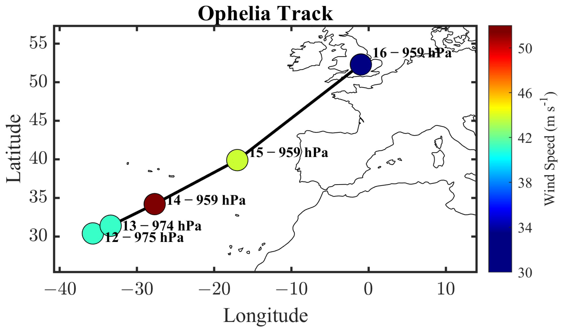
The intensity of Ophelia peaked on 14 October, with a minimum central pressure of 959 hPa and a maximum sustained wind speed of 51 m s−1 (Figure 3). Ophelia was steered into the wIP ahead of an upper-level trough from the southwest, weakening as it passed over a cooler area of SST at 23 °C, and higher wind shear. By 00:00 UTC, on the 16th of October, it had already transitioned into an extratropical cyclone with a maximum sustained wind speed of 38 m s−1 [62].

Figure 3.
Tropical cyclone Ophelia’s best track position, minimum central pressure, and maximum sustained winds at 12 UTC between 12 and 16 October 2017 [62].
Over continental Portugal, on the 14th of October 12 UTC, the analysis made by IPMA of the vertical soundings acquired at Lisbon showed a dry layer below 700 hPa, with an inversion layer underneath. At middle-high levels, a high moisture flow was advected over the dry layer, resulting in a high LCL. From the 14th to the 15th of October, the LCL height increased to 670 hPa. An inverted V profile was present on both the 14th and the 15th of October, with CAPE reaching values close to zero [38].
Warm and dry air advection from Ophelia resulted in very low fine fuel moisture contents, with values as low as 5%. Strong wind gusts from Ophelia’s circulation (30 km h−1 wind speed, 50 km h−1 wind gust speed in the study area) in conjunction with low fuel moisture values and the effect of exceptionally long drought promoted an extreme Fire Weather Index ranging between 50 and 85 [31].
3.2. Large Scale Model Results
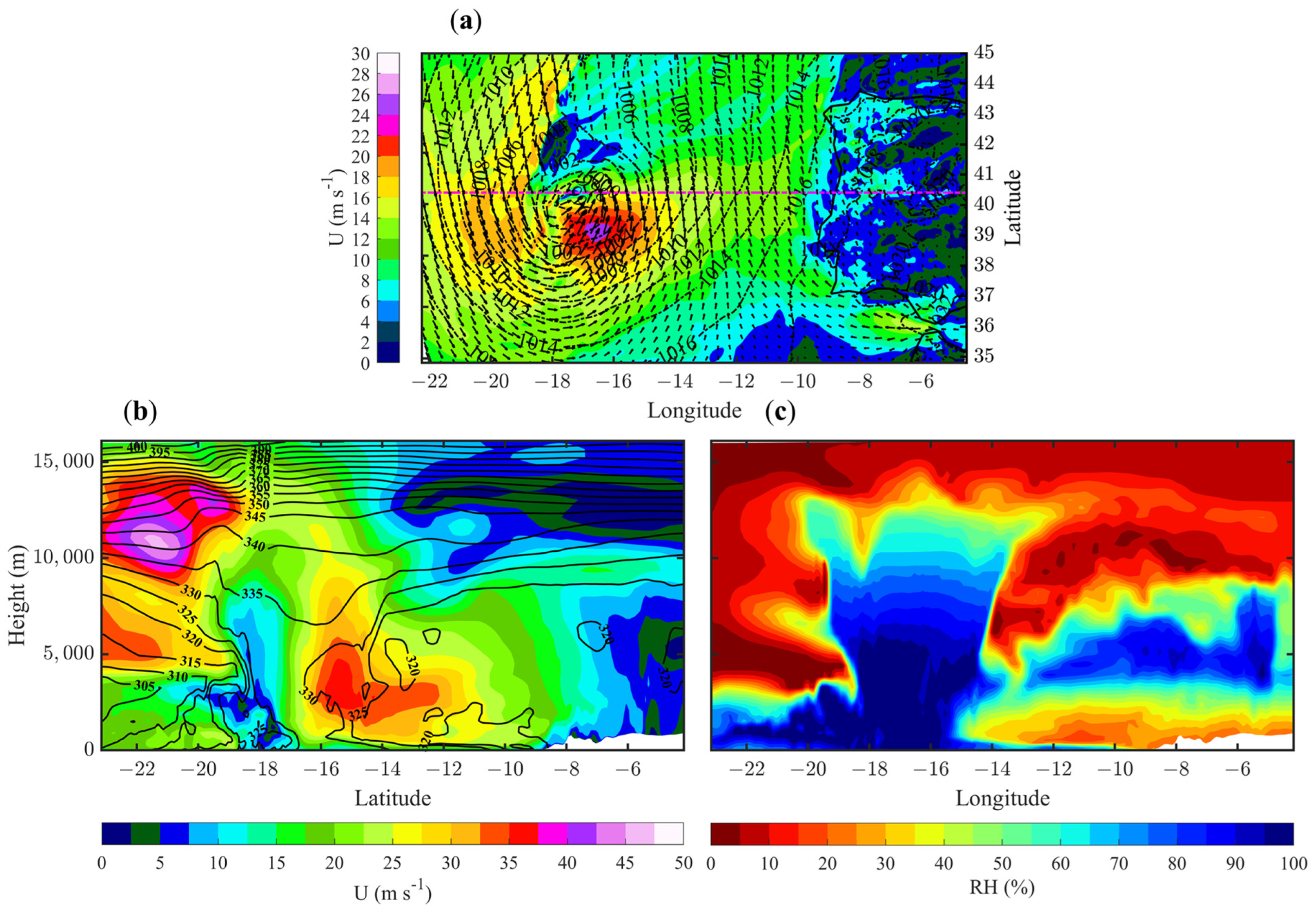
Figure 4 shows a synoptic analysis of the model results from d01 on the 15th of October at 12:00 UTC. The simulated minimum sea level pressure (mslp) is 995 hPa with maximum surface wind speeds of 25 m s−1 (Figure 4a). This is an underestimation compared to best track data, which reports a central pressure of 959 hPa and maximum sustained winds of 43.7 m s−1. Over continental Portugal, wind speeds range between 2 and 8 ms−1, reaching values of 8–10 ms−1 over central mountainous regions. Very small to no CAPE values were observed over land from the simulation outputs, which is corroborated by the vertical sounding observations [38]. Figure 4b shows a vertical cross-section of wind speed, taken along the dashed purple line in Figure 4a. A wind maximum of 36 ms−1 is seen on the westward flank of the tropical cyclone, at 3000 m height above mean sea level (a.m.s.l.). To the west, the high-level trough that steered the cyclone, Figure 4b dashed, is observed ahead of the jet stream. A maximum equivalent potential temperature, θe of 320 K is observed at the surface, extending up to 7000 m a.m.s.l. Eastward of the tropical system, a large area with a neutral or small θe vertical gradient (Figure 4b contours) extends from the cyclone’s centre to deeper inland, indicating a potentially neutral unstable atmosphere [63]. Westward from the trough, a broad area of cooler and drier air follows the low-pressure system (Figure 4c).
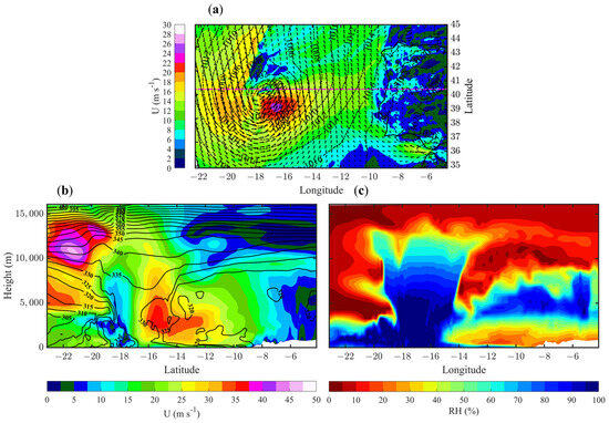
Figure 4.
Tropical cyclone’s horizontal and vertical synoptic structure in d01, on the 15th of October 2017 at 12:00 UTC. The figure panels represent: (a) Surface pressure field in black contours, 10 m wind vectors as black arrows, 10 m wind speed in shaded colours, and the zonal magenta line at 40.5° N showing the location of the vertical cross sections depicted in panels (b,c); (b) vertical wind speed in shaded colours and potential equivalent temperature in black contours, and the position of the shoreline indicated by the black arrow; (c) vertical cross section of RH in shaded colours, with dashed black rectangle highlighting the high moisture air advected into the tropospheric mid-levels, and the solid black rectangle highlighting the dry air mass advected into the low tropospheric levels.
The influence of Ophelia on vertical RH is observed up to 14,000 m a.m.s.l. Eastward of the cyclone, a warm and dry layer is advected within the first 3000 m a.m.s.l. (bold rectangle, Figure 4c), responsible for the fire-prone atmospheric conditions at the surface. Above this dry/warm layer is a moist layer that extends up to 8000 m a.m.s.l. (dashed rectangle, Figure 4c). These conditions produce the “inverted V” vertical profile referred by the IPMA report, as can be seen in the vertical soundings in [38]. The cyclone displays an asymmetrical wind structure at the surface, with the strongest winds being seen in the eastern flank of Ophelia (Figure 4b), breaking up to the north-northwest as it began to undergo the extratropical transition [62].
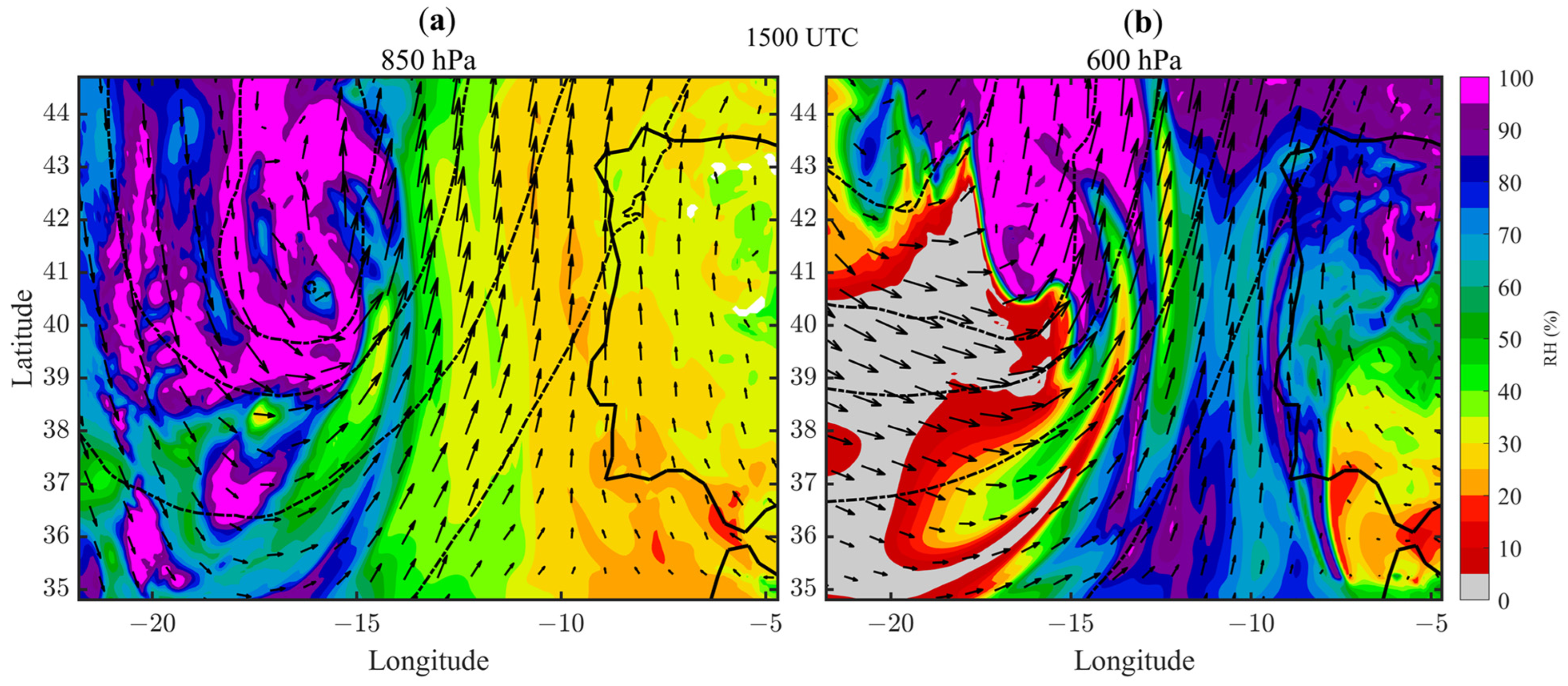
RH at 850 hPa and 600 hPa is shown in Figure 5. In Figure 5a, at 850 hPa, Ophelia still displays a closed ring of clouds around the centre as it is steered northeast, with its circulation advecting dry air (20% to 30% RH) over the IP. At 600 hPa, the opposite occurs, and very dry air intrudes the cyclone from the southwest, behind the trough as a moist air flow (up to 95% RH) is carried over Portugal.
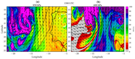
Figure 5.
Wind arrows, geopotential height contours, and shaded RH of Ophelia are displayed for the pressure levels of 850 hPa (a) and 600 hPa (b), showing the dry air advection a the surface, and southern moisture flow aloft.
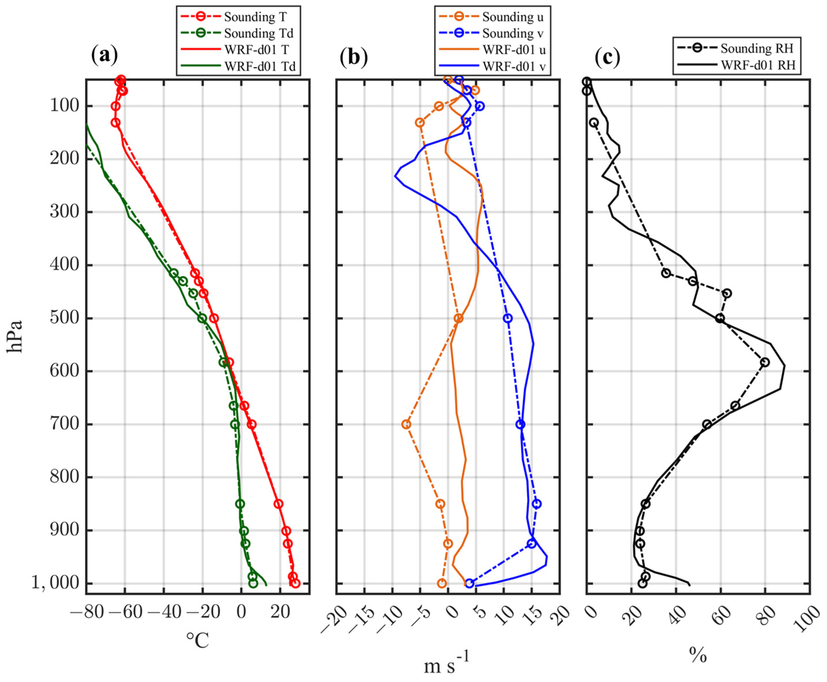
Figure 6 shows a comparison between a simulated vertical profile, and vertical sounding observations, on 15 October at 1200 UTC, in Lisbon (red star, Figure 1). The simulated temperature and dew point temperature (Td), in Figure 6a, and RH, in Figure 6c, are in good agreement with observations in the 1000–600 hPa layer, with an underestimation of RH (−5%) at 900 hPa. Levels between 600 and 500 hPa show an overestimation of Td/RH (+10 to +15%), and an underestimation above 500 hPa (−5 to −20%). The northward wind component (v) and eastward wind component (u), Figure 6b, were well represented in the simulation at all levels, with minor differences in u near the surface and aloft, at 700 hPa.
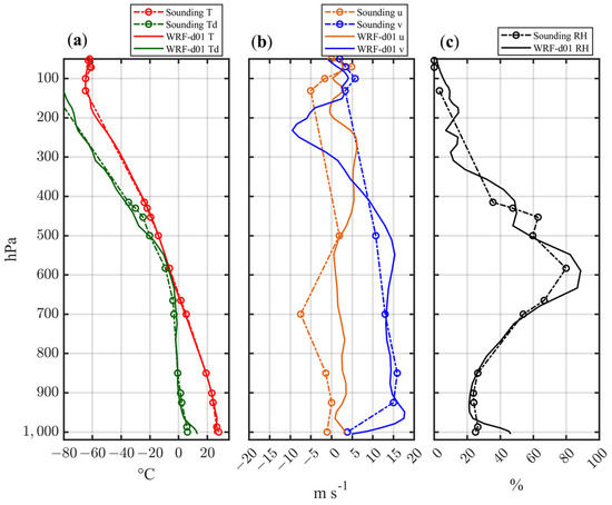
Figure 6.
Lisbon vertical sounding comparison (dashed) with d01 simulation results (bold): panel (a) displays vertical temperature (red) and dewpoint temperature (green); panel (b) shows the u wind component (orange) and v wind component (blue); and panel (c) shows RH.
3.3. Surface Weather Analysis
Weather station data is compared in Figure A1, Figure A2, Figure A3 and Figure A4 of the Appendix A, showing temperature, RH, wind speed and wind direction comparisons with d02, d03 and d04-LES model results, on the 15th of October, between 09:00 and 18:00 UTC. For reference, a topographical map showing the stations locations is displayed in Figure 7. Temperature (Appendix A, Figure A1) and RH (Appendix A, Figure A2) are well represented at all weather stations in d02. The coastal weather stations of Figueira da Foz and Dunas de Mira show the largest deviations from observations, with lower simulated RH. Only the station of Figueira da Foz overestimates the temperature, by approximately 2 °C between 10:00 and 15:00 UTC. Lousã weather station shows the greatest overall differences in RH (+ 7.5%) and temperature (−2 °C) due to its proximity to complex terrain. The WRF model has been shown to perform less effectively in those conditions [64]. Regarding wind speed (Appendix A, Figure A3), it is either well represented or largely overestimated, in the case of Anadia, Ansião and Dunas de Mira by 4 ms−1, apart from Figueira da Foz where wind was underestimated between 11:00 and 15:00 UTC. The wind direction (Appendix A, Figure A4) shows agreement with the observations, except for the station located at Dunas de Mira. All coastal weather stations seemed to capture the wind direction change, from S/SE to SW observed at 15:00 UTC, accompanied by a sharp reduction in temperature and an increase in RH at the correct timeframe [38], coinciding with the moment when coastal fires became predominantly convection-driven instead of wind-driven [29].
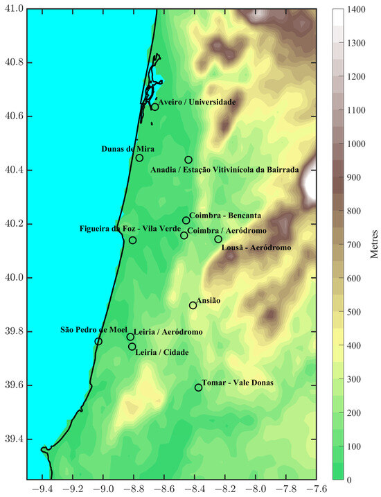
Figure 7.
Location of the weather stations used for validation within d02, overlaying shaded topography.
Despite showing good performance in d02, the higher resolution simulations in d03 and d04-LES fails to represent the rise in humidity and the sharp reduction in temperature observed at 15:00 UTC. In d03, the hourly temperature profiles are similar for Dunas de Mira and Figueira da Foz, the two closest weather stations to the study area, but after 15:00 UTC, small increases/decreases are observed in either of the two stations for RH and temperature, respectively. The effect of the turning wind in advecting cooler and higher moisture oceanic air is not represented by the model at these resolutions. The simulated temperature at Figueira da Foz is closer to observations; however, in d04-LES, this discrepancy is much larger than in d03. The temperature peaks at 12:00 UTC and from then on begin its slow descent, which contrasts with the sharp descent observed at coastal stations.
3.4. Model Sounding Analysis
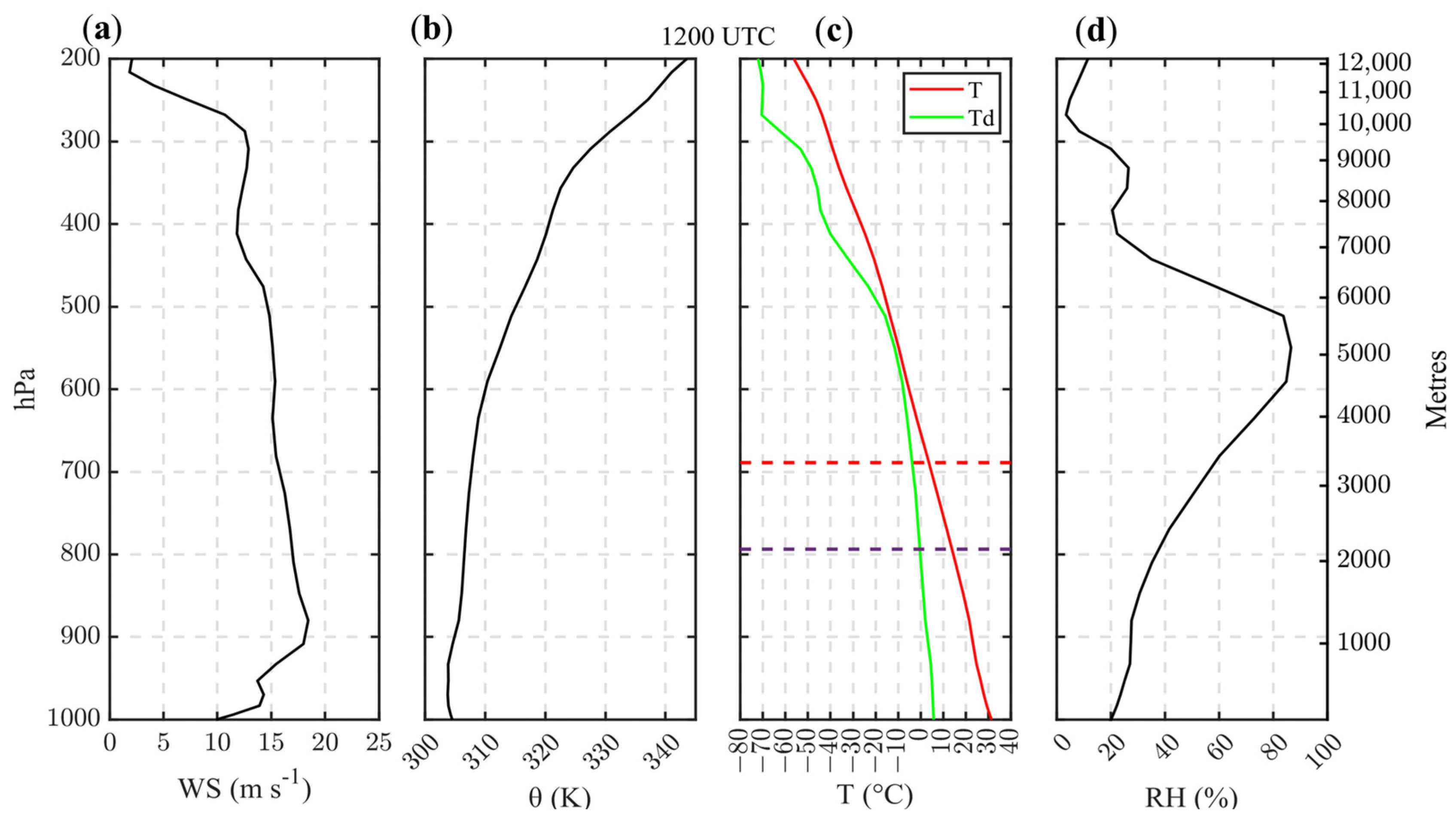
Figure 8 shows a vertical profile extracted at 12:00 UTC from d04-LES over the fire ignition location, indicating the presence of a low-level jet (LLJ) above 900 hPa, which was also observed in modelled vertical profiles taken later at 15:00 UTC [38]. The potential temperature gradient is minimal in the 600–1000 hPa layer, showing near neutral static stability aloft. Dry and hot low levels contribute to a high LCL, above 700 hPa, with the top of the PBL just below 800 hPa. The “inverted V” profile is still reproduced in the d04-LES domain with RH values higher than 80% simulated between 500 and 600 hPa.
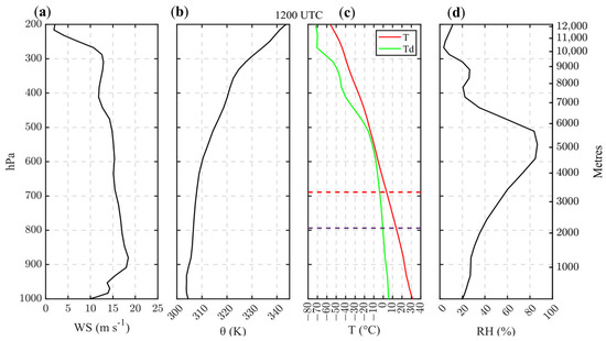
Figure 8.
Vertical sounding extracted from the d04-Les simulations. Panels (a–d) show wind speed, potential temperature, temperature (red) and dewpoint temperature (green), and relative humidity. LCL height and PBL height, from Equation (2) are shown in dashed red and dashed purple, respectively.
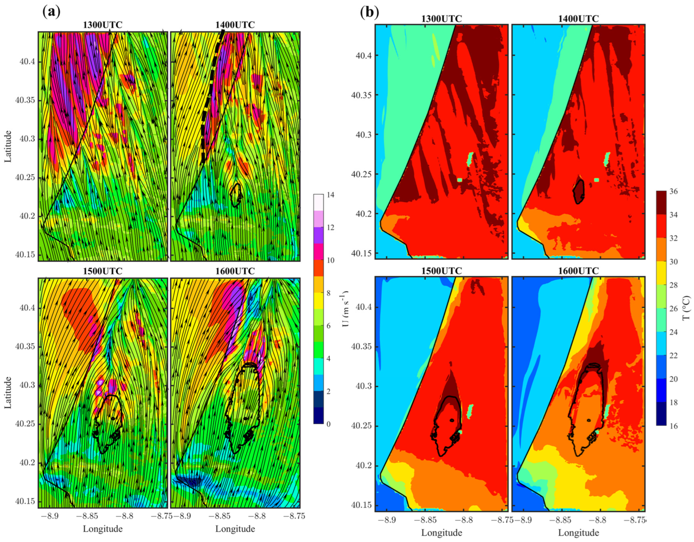
Figure 9 shows the simulated surface wind speeds, wind streamlines, and surface temperature at four different times: 13:00 UTC, preceding the fire, and the remaining times after fire initiation. At 13:00 UTC, the presence of horizontal convective rolls is shown as zones of convergence and divergence at the surface. Convergent zones present lighter wind speeds converging with divergent, increased wind speeds. The southeastern flow extends deeper into the ocean at this instant. At 14:00 UTC, the horizontal rolls deform under the presence of fire and shifting winds, and a convergent zone is seen forming west of the coastline as winds begin to shift. At 15:00 UTC, the wind speed increases along the fire front, 9–13 m s−1, and a convergence zone is formed downstream. At this time, the horizontal convective rolls cease, and the winds weaken south of the fire area. At 16:00 UTC a forked convergence zone surrounds the flanks of the fire, merging north. Winds along the shoreline increase to 13 ms−1, together with fire-induced winds downstream of the fireline.
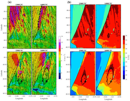
Figure 9.
In (a) four panels show wind streamlines and, shaded, 10 m wind speed at 4 distinct moments of the wildfire. The top left panel illustrates the pre-fire surface and the dashed black line in the top right panel shows the convergence zone created by the wind direction shift. (b) illustrates the same moments, with temperature at 2 m shaded.
3.5. Thermodynamics of the Plume
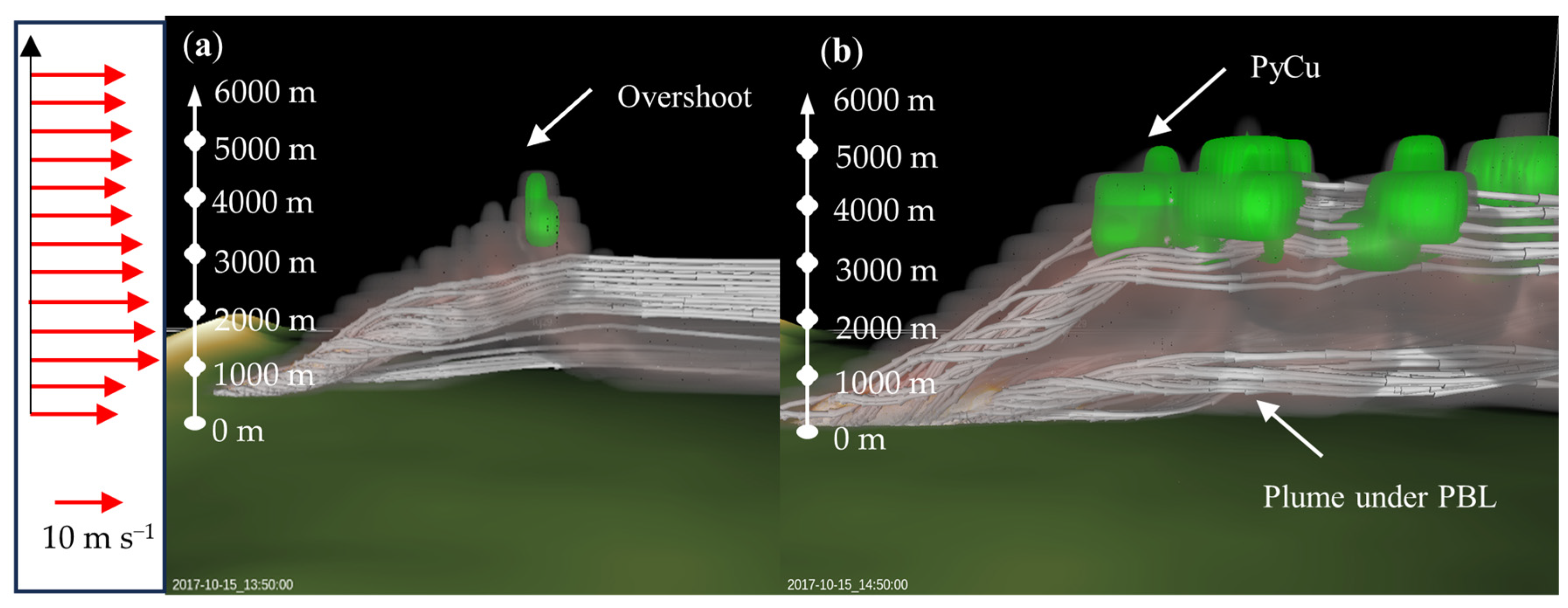
A 3D view of the fire plume, in Figure 10, shows two different moments of the fire. Figure 10a shows the initial moments of the fire at 13:50 UTC. At this stage, the wind streamlines began to split into two different levels: a lower level situated above the LLJ, underneath the top of the PBL, and a plume overshooting, producing a small PyCu. This was, in fact, observed initially via photographs [31], highlighting the high intensity that developed early in the fire. Figure 10b shows further penetration of the fire plume through the PBL and a widespread formation of PyCu downstream, with a maximum vertical extension of 2 km. These forms of pyroconvective behaviour are explained by [12], who analyse the thermodynamics of several wildfire pyroconvection events. The vertical dispositions of the wind shear, LCL, and PBL top, observed in the simulations of the Quiaios fire, are also compatible with the overshooting profile described by the authors, with a flattened plume along the vertical wind shear maxima, underneath the PBL top, and the LCL aloft. This is otherwise observed for most of the simulation time, with several PyCu generated at the leading edge of the fire plume top and a second lower-level plume underneath the PBL top. Notably, the streamlines also show how the plume rises in a corkscrew motion, suggesting a vortex like structure on the vertical plane.

Figure 10.
VAPOR 3D visualisation of the fire plume using WRF-SFIRE’s smoke tracer (reddish grey) at 13:50 UTC, left panel (a); and 14:50 UTC, right panel (b). Cloud hydrometeors are coloured in green, and wind streamlines in white. The left panel (a) shows the overshooting plume creating a small PyCuMore prevalent pyroconvection is shown on the right panel (b). Red arrows on the left show the vertical wind speed taken at the ignition point at 12:00 UTC, for each designated height on the scale.
3.5.1. Fire Circulation’s Effect on the LLJ and Plume Geometry
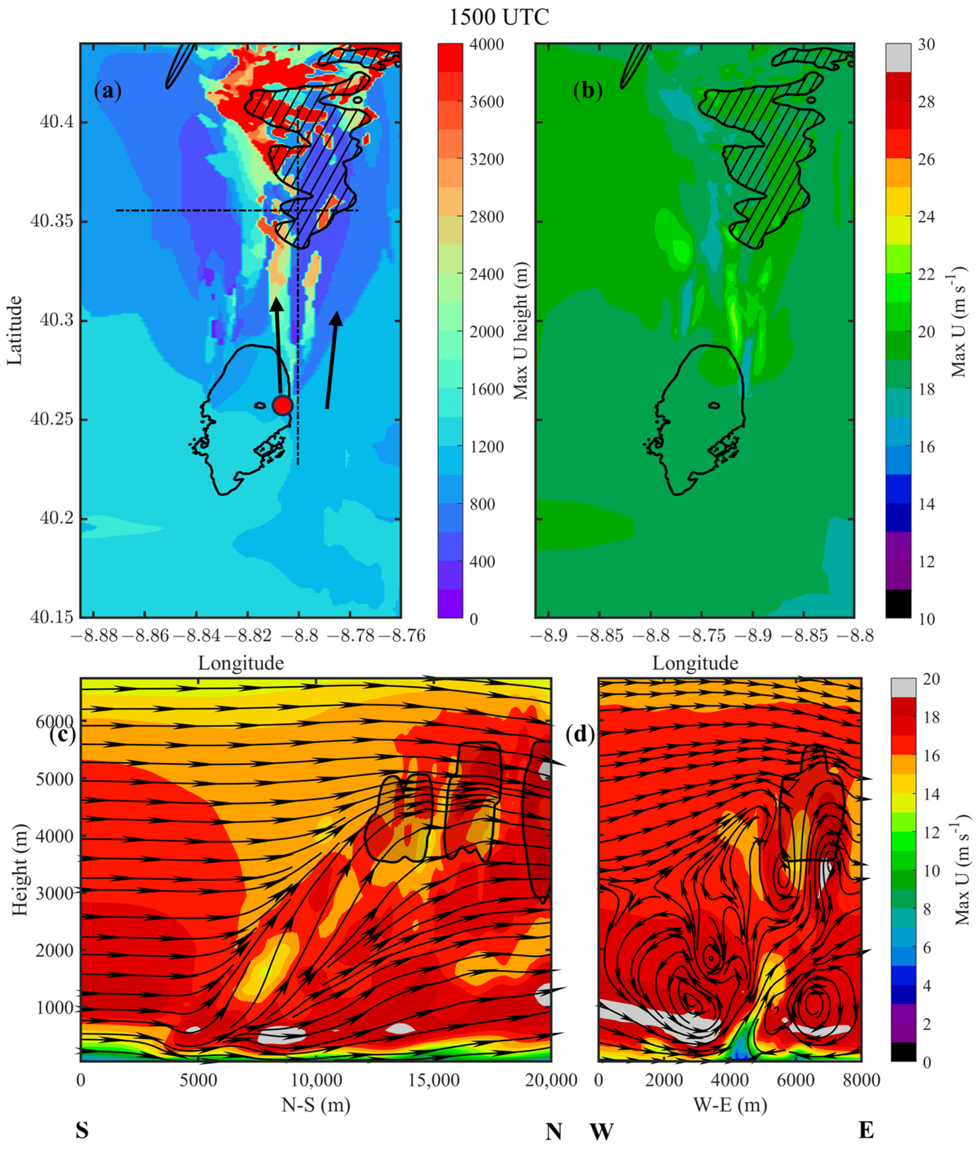
To understand in more detail the effects of the fire on the surface, the vertical wind dynamics and the LLJ, the maximum wind speed height was retrieved from d04-LES model results and its magnitude determined. Figure 11a,b show two parallel maximum wind speed heights and magnitude signatures downstream of the fire head, displayed along two line-like structures, between 2 and 3 km in height or roughly 1 km above the low-level jet position (~1 km in height). Along these lines, the simulated winds observed were 2–3 m s−1 above the 19 m·s−1 LLJ. Furthermore, out of these structures, a diminishing maximum wind speed height, of 200–500 m, occurs along a broad area above and downstream of the fire, highlighting the effect of fire-induced circulation in lowering the LLJ closer to the surface, thus promoting the fire spread. This circulation resembles the concept by Potter [65], who idealised the structure of wildfire circulation as an indraft over the fire and a return downward flow spread horizontally aloft. However, the circulation of the Quiaios fire differs from Potter’s concept, which was conceptualised for a no-wind atmosphere, in that the fire plume is heavily tilted downstream, as shown in Figure 11c. In this case, we can see how the updraft base and top, where PyCu has formed, are horizontally displaced by approximately 7 km. Pyroconvective clouds are shown to form downstream of the fire head (black hatched) approximately 7 km apart. It should also be noted that the zonal cross section is 9 km away from the fire head, and despite the distance, it shows that the general updraft and return downdraft convective structure stretches far beyond the fire’s location and is most likely responsible for the spiralling wind streamlines shown in Figure 10. At the centre of the updraft, the winds are lighter at the surface, as shown in Figure 11d. The structure of the updraft is also tilted zonally when comparing the 15:00 UTC cross sections to the surface results shown in Figure 11. The convergence zone at the surface is still present in Figure 11c, shifted westward of the fire head, which is also visible in Figure 11d, where the vertical wind streamline is displaced eastward from the surface by 2 km. The wind speed maxima occurring above the jet height suggest that the wildfire’s updrafts carry the circulation upwards and downstream.

Figure 11.
In panel (a), the maximum wind speed height is coloured and the surface fireline is shown in bold. The red circle signals the position of the fire head, and the arrows show the two maximum wind height structures formed by the fire circulation. The lightly shaded black contour shows the location of the clouds on the horizontal plane. The two dashed lines indicate the positions of a zonal and meridional cross section and will henceforth be used as reference for every other meridional and zonal cross sections. Panel (b) displays the maximum wind speed at the height from panel (a). Panels (c,d) show the meridional and zonal cross sections from (a), respectively, maximum wind speed in shading and wind streamlines on the respective planes. Cloud area is defined in bold black contour lines.
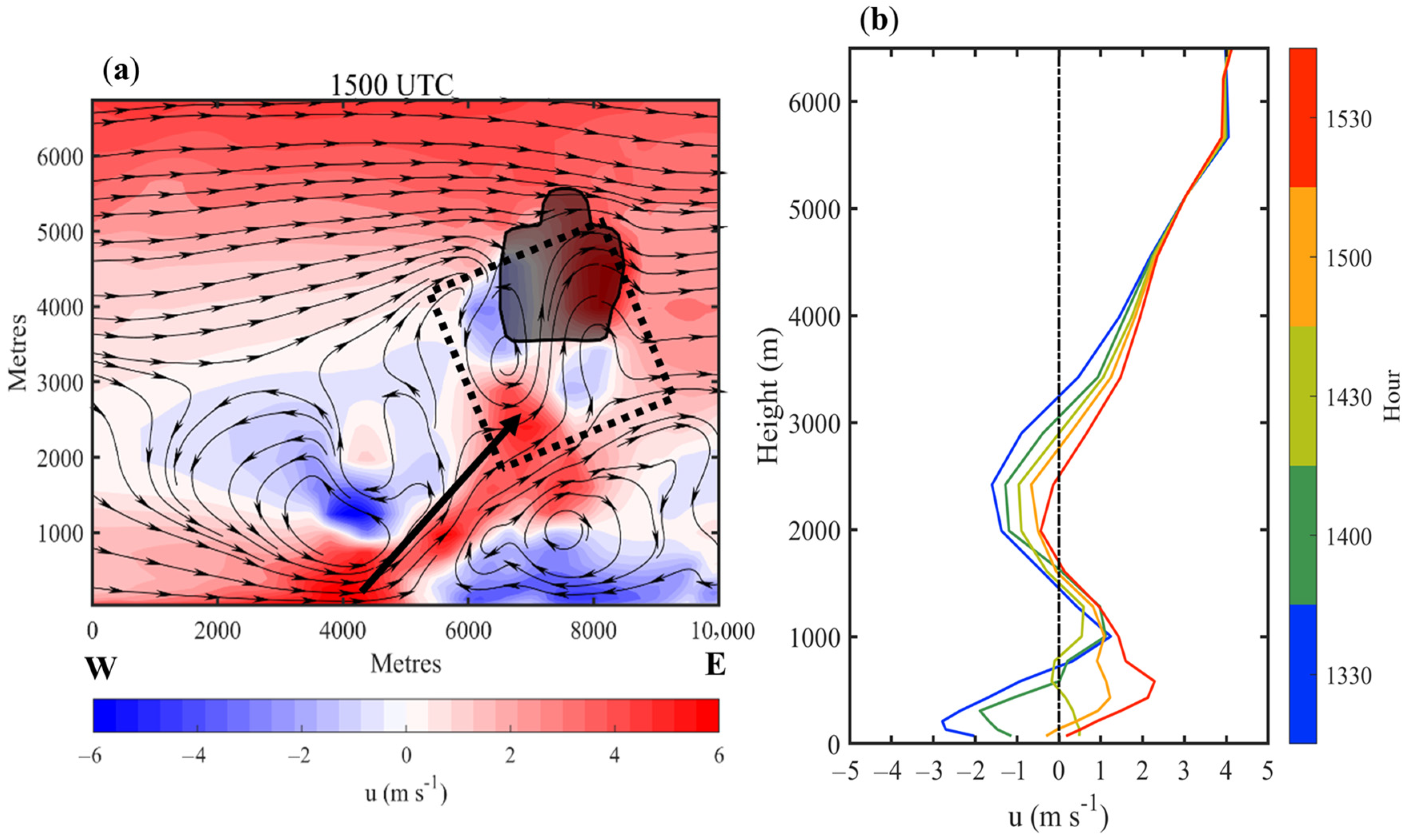
The same zonal cross-section as that in Figure 11a is shown in Figure 12a, displaying the zonal wind component, u. In Figure 12b, the u component vertical profiles from a no-fire simulation of d04-LES are shown. Similarly, the zonally tilted updraft is indicated by the black arrow. In Figure 12a, at the surface, the left side of the indraft is stronger than the right side, most likely enhanced by the changing wind directions between 0 and 1500 m, as shown in Figure 12b, and discussed in Section 4. Aloft, similar vortex structures are shown with the updraft entering the PyCu.
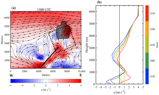
Figure 12.
A zonal cross section, taken from Fi gure 11a shows (a) the shaded u wind component and wind streamlines. The black arrow highlights the tilt of the fire’s updraft leading into a PyCu cloud, in dark shading. The same structure of surface convergence and upper diverging winds is shown aloft by the dashed square. In (b), the environmental u wind component is taken from the no fire simulation, at 5 different coloured periods, to highlight the change in wind direction near the surface.
3.5.2. Thermal Differences Between Fire and No-Fire Simulations
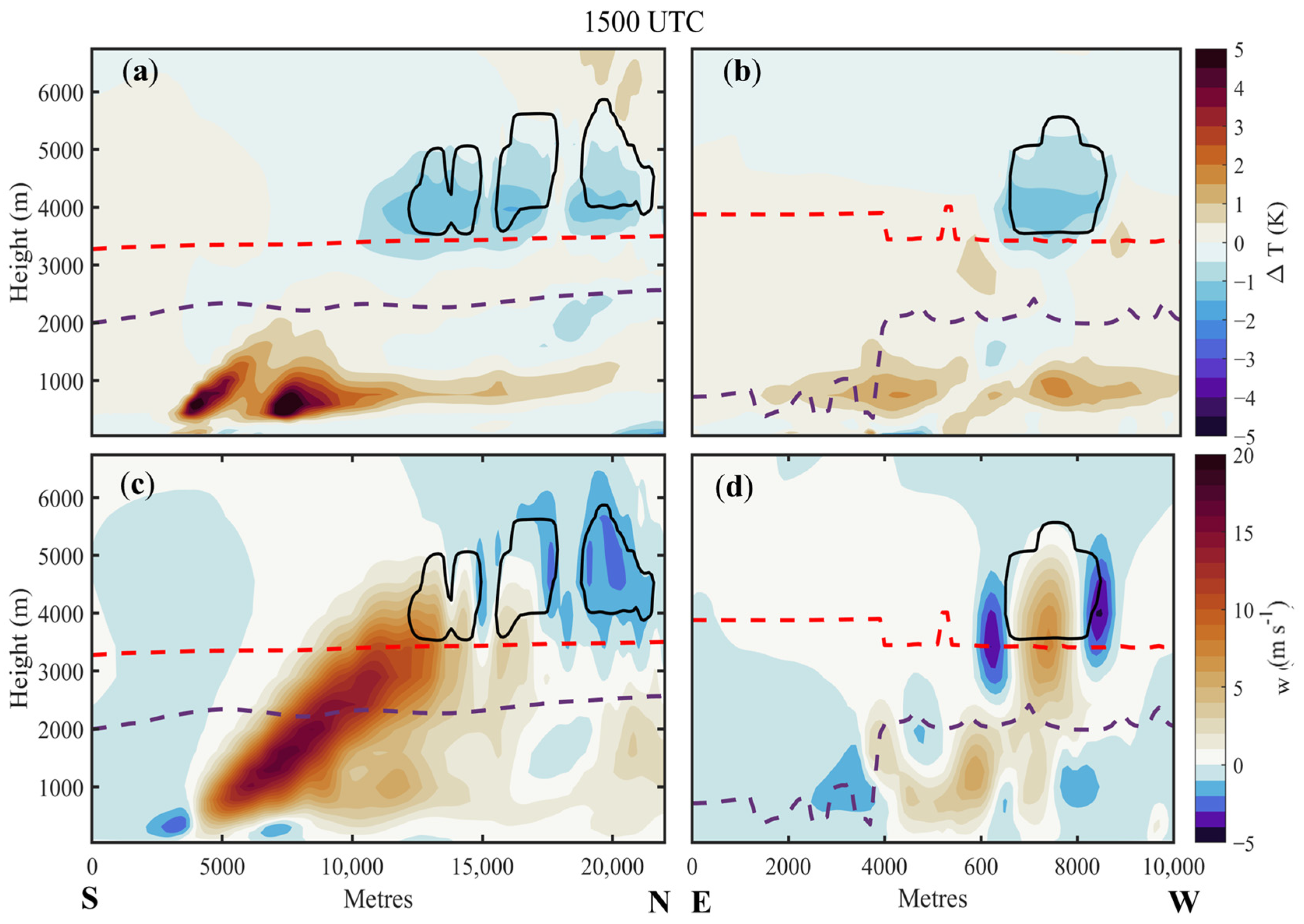
The differences between the environmental and fire vertical temperatures are shown in Figure 13a,b. The effect of sensible heat fluxes on the atmosphere showed a temperature anomaly within the near surface environment of +7 K, at 800 m. Note that this cross section is displaced a few hundred metres east of the fire head in order to capture the tilted plume of the fire.
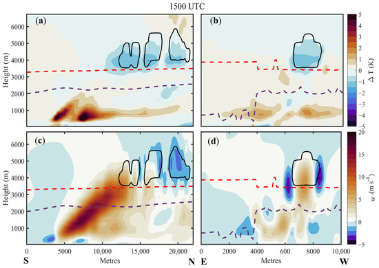
Figure 13.
Coloured differences in the temperature between the fire and the environmental simulations are shaded the upper panels (a,b), and the vertical wind speed is shaded in (c,d). Red dashed lines show the environmental LCL, and the purple dashed ones the PBL height. The cross sections are taken across the constant N–S, W–E lines shown in Figure 11a.
Above the PBL top, sensible heat fluxes no longer register any change in the atmosphere. The meridional tilted updraft in Figure 13c shows a maximum vertical wind speed of 18 m s−1 in this cross section. Once again, the cross section position is not favourable to observing the strongest updrafts, which range as high as 25 m s−1 at 1420 UTC, preceding this period of pyroconvection in the simulations. The maximum updraft speed is located approximately 500 m above the maximum temperature anomaly and soon begins to slow down to 5 m s−1 as it reaches the first PyCu. Simulations by Luderer et al. (2006) and Trentmann et al. (2006) of a large pyCb producing fire in Canada show how the temperature anomalies from the fire decay quickly with height, and how the maximum updraft speed is located near the surface fire, highlighting the importance of sensible heat fluxes in initiating convection [13,21]. Generally, Figure 13a shows an almost continuous extension of PyCu formed above the LCL (red dashed line) at 3500 m. The PyCu located directly above the updraft have a cloud base closer to the LCL, while downstream they possess a higher cloud base height, at around 4000 m. A temperature anomaly is also visible underneath them, diminishing as it approaches the top of the PyCu cloud. The PyCu further away from the top of the fire’s updraft are associated with descending movements.
3.5.3. The Effect of Fire on Atmospheric Stability and Water Vapour Transport
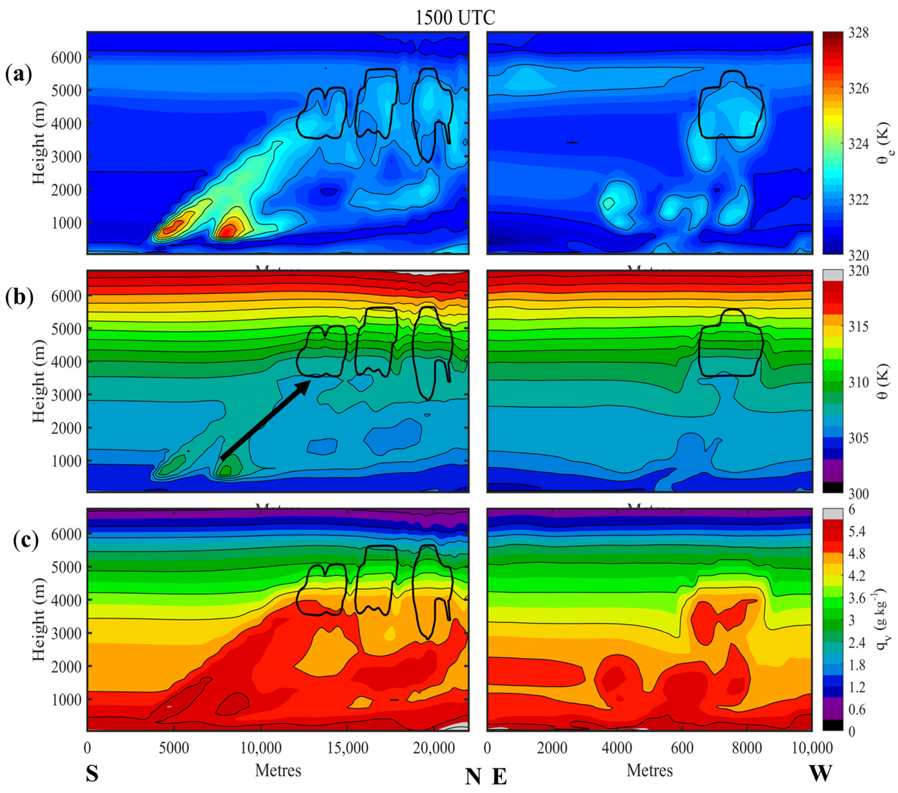
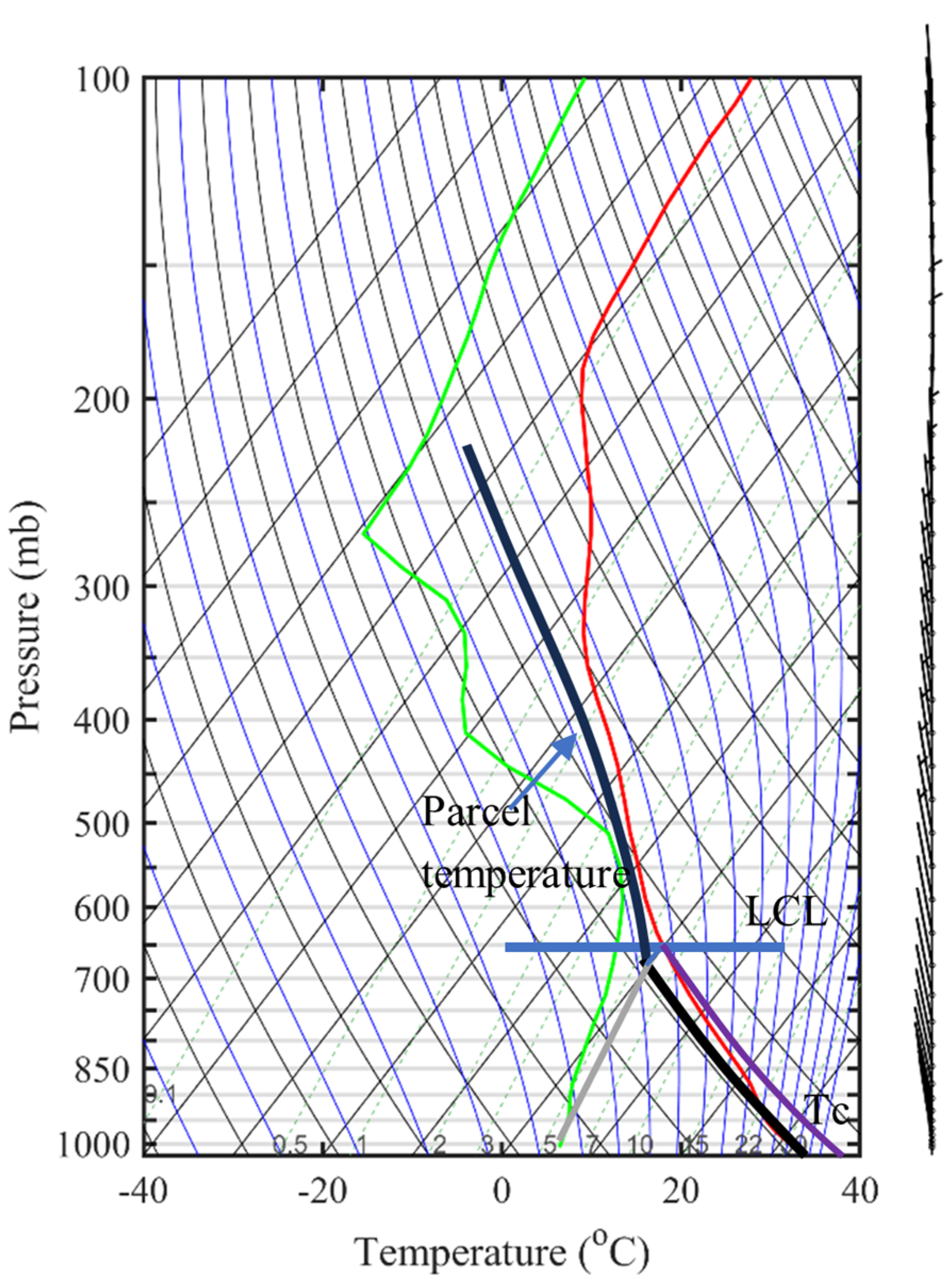
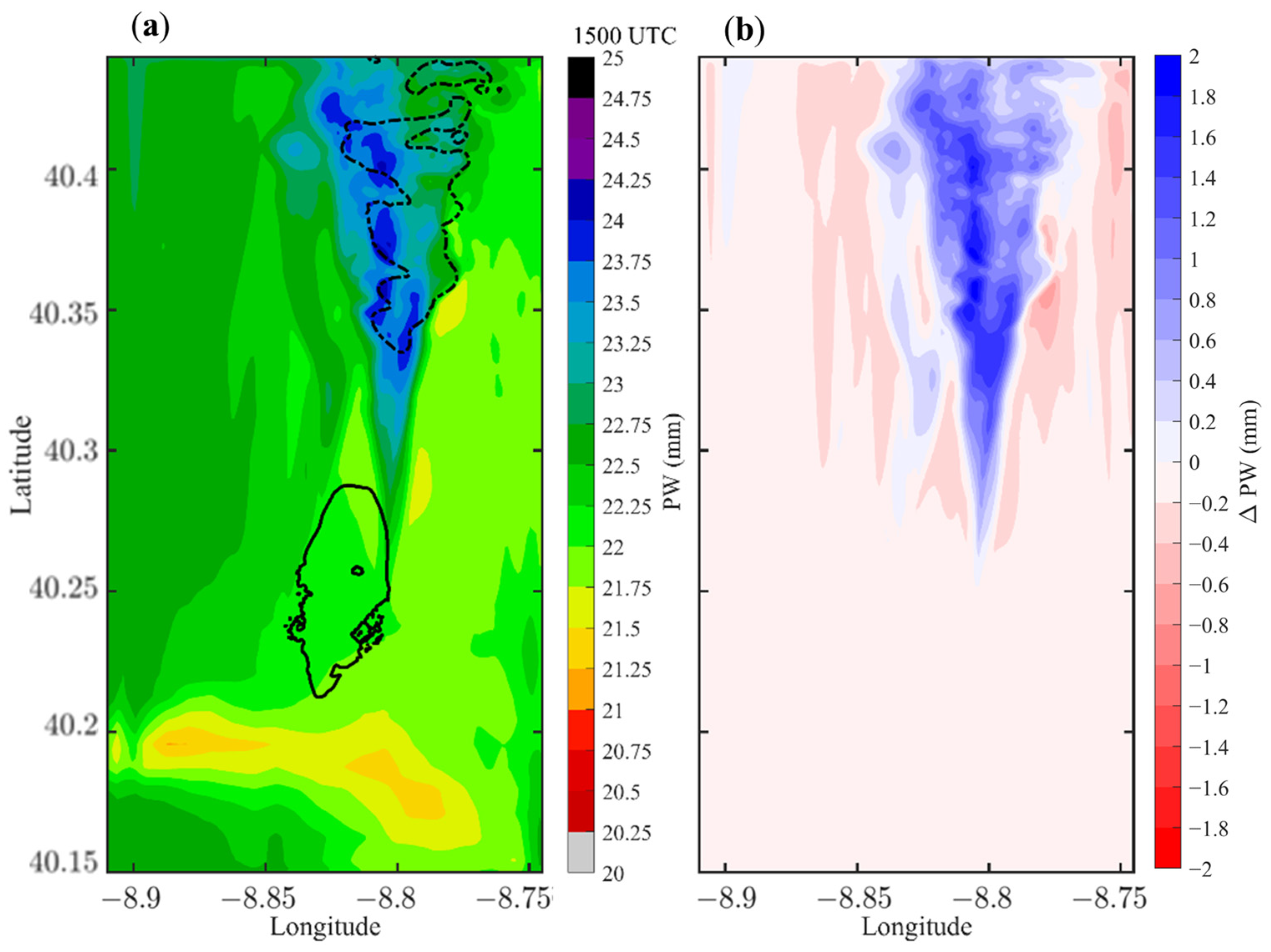
Figure 14 depicts the zonal and meridional cross-sections of equivalent potential temperature (θe), potential temperature (θ), and water vapour mixing ratio (qv). In Figure 14a the highest potential temperature is shown near the surface where θ and qv are maximum, and where the sensible heat flux from the fire is most intense. As described previously, plume dilution via environmental entrainment lowers the rising updraft equivalent temperature, θ, and thus its buoyancy. Furthermore, the effect of high wind speeds and turbulence on tilting the plume further decreases its buoyancy as it is flattened to the horizontal plane, as shown previously in this wildfire (Figure 10 and Figure 11) [9]. At the top of the updraft, θ is lower than the surrounding environment by ~1 K (Figure 14b), and is negatively buoyant, as shown by in Figure 13a,b. Despite having a lower θ, the θe of the parcel is higher than that of the surrounding environment and would have had the potential to become positively buoyant if enough latent energy would be released by condensation, which does not seem to be the case, as further downstream parcels are producing downdrafts, likely to be associated with the sinking of the lifted denser air, but also by evaporative cooling of the small PyCu cloud. Moreover, an inversion of θe was observed above 5000 m, reinforcing the stability of this level. As stated previously, the CAPE in this profile is zero, as shown by the lifted parcel trajectory obtained from the environmental profile in Figure 15. Water vapour with a mixing ratio of 4.5 g kg−1 (qv) was transported vertically from the surface (Figure 14c), along the updraft, to as high as 4000 m, which can also be traced by the higher θe aloft, despite lower or equal θ at the same level. It has also been shown that the burning of fuel in forest fires contributes to the addition of moisture in the vicinity of the fire, which can also be seen in PW fields of the simulation of the Quiaisos fire in (Figure 16a), where an increase of 1.5–2 mm when compared to the environmental run is detected. References [13,21] refer in their model studies that the total contribution of the water vapour from fires above 4000 m is less than 10% of the total water in the plume. In this study’s scenario, the total water vapour contributed by the fire is, at best, 6–8% of the total vertical qv, which, despite not being a direct comparison, would still fall in line with the assumption, given how quickly the plume diluted before reaching the LCL (Figure 14a). The variability of moisture released by the fire could possibly be altered by having wetter burning fuels, but surface fuel dryness is linked to the atmospheric conditions of heat and moisture.
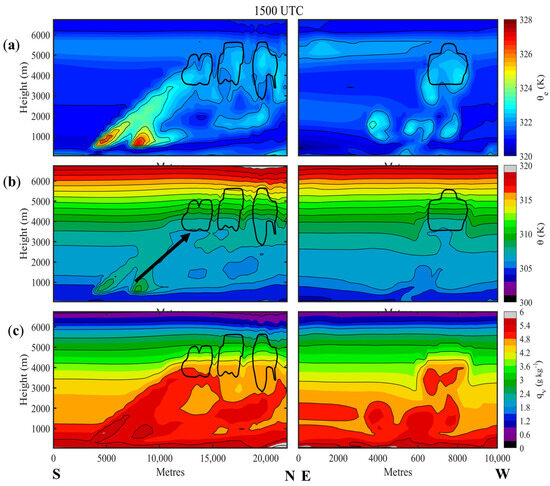
Figure 14.
Three sets of cross sections are shown, taken across the constant N–S, W–E lines shown in Figure 11a. PyCu positions on the cross section are contoured in black. The meridional cross section is shown on the left, and the zonal on the right. Shaded θe is illustrated in (a), θ in (b), and water vapour mixing ratio, qv, in (c).

Figure 15.
Skew-T thermodynamic profile of the 1200 UTC fire ignition point showing the temperature (red), dewpoint temperature (green) and the lifted parcel temperature in deep black. The LCL height is shown in dark blue and the temperature for convection initiation (Tc) in purple.

Figure 16.
Integrated precipitable water is shaded in panel (a), fire perimeter in black contours and pyroconvective cloud position in dashed black contours. Panel (b) illustrates the difference in precipitable water between the fire and the environmental simulations.
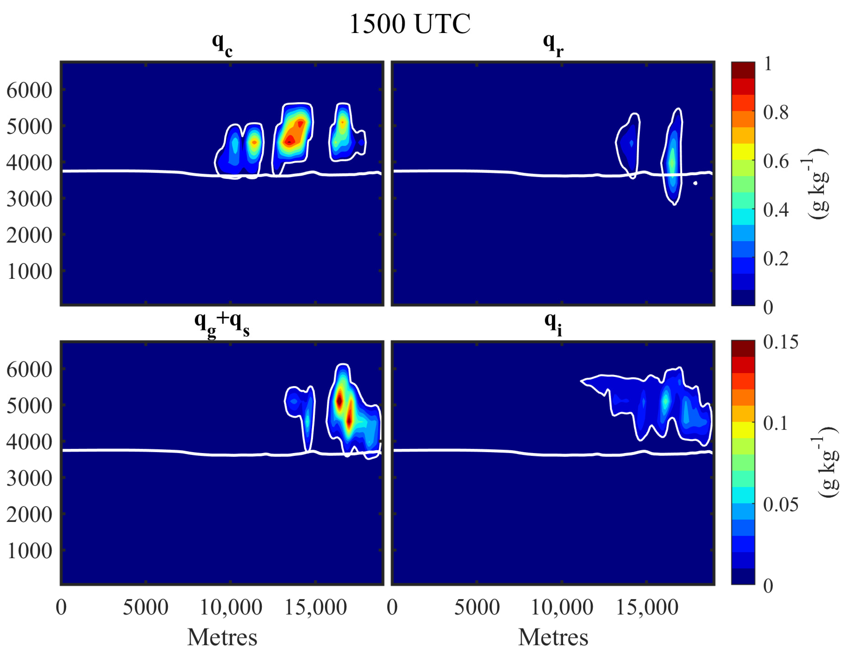
3.5.4. Composition of the Simulated Pyroconvective Clouds
In Figure 17, we look into the different hydrometeor species present in the PyCu structure, divided into four species: cloud water mixing ratio qc, rainwater mixing ratio qr, graupel and snow mixing ratios qg + qs, and finally, ice mixing ratio qi. The specie with the highest concentration is qc, with up to 1 g kg−1. The remaining hydrometeors occur at concentrations up to seven times smaller. Rainwater mixing ratios are the second highest, reaching 0.5 g kg−1. As stated previously, the strongest updraft (~25 m s−1) occurs at 14:20 UTC, but more developed clouds, with all hydrometeor species, present the highest mixing ratio at 15:00 UTC. A downdraft formed underneath a PyCu, with a maximum qr of 0.4 g kg−1 and wind speed of −3 m s−1, occurring at 14:30 UTC (Appendix A, Figure A5).
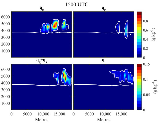
Figure 17.
Shaded hydrometeor species are divided in the four panels, across Figure 11a’s meridional section. Top left panel—cloud water mixing ratio (qc); top right panel—rain water mixing ratio (qr); bottom left panel: snow and graupel mixing ratios (qg + qs); bottom right panel—Iie mixing ratio (qi). The freezing level (T = 0 °C) is displayed in bold white.
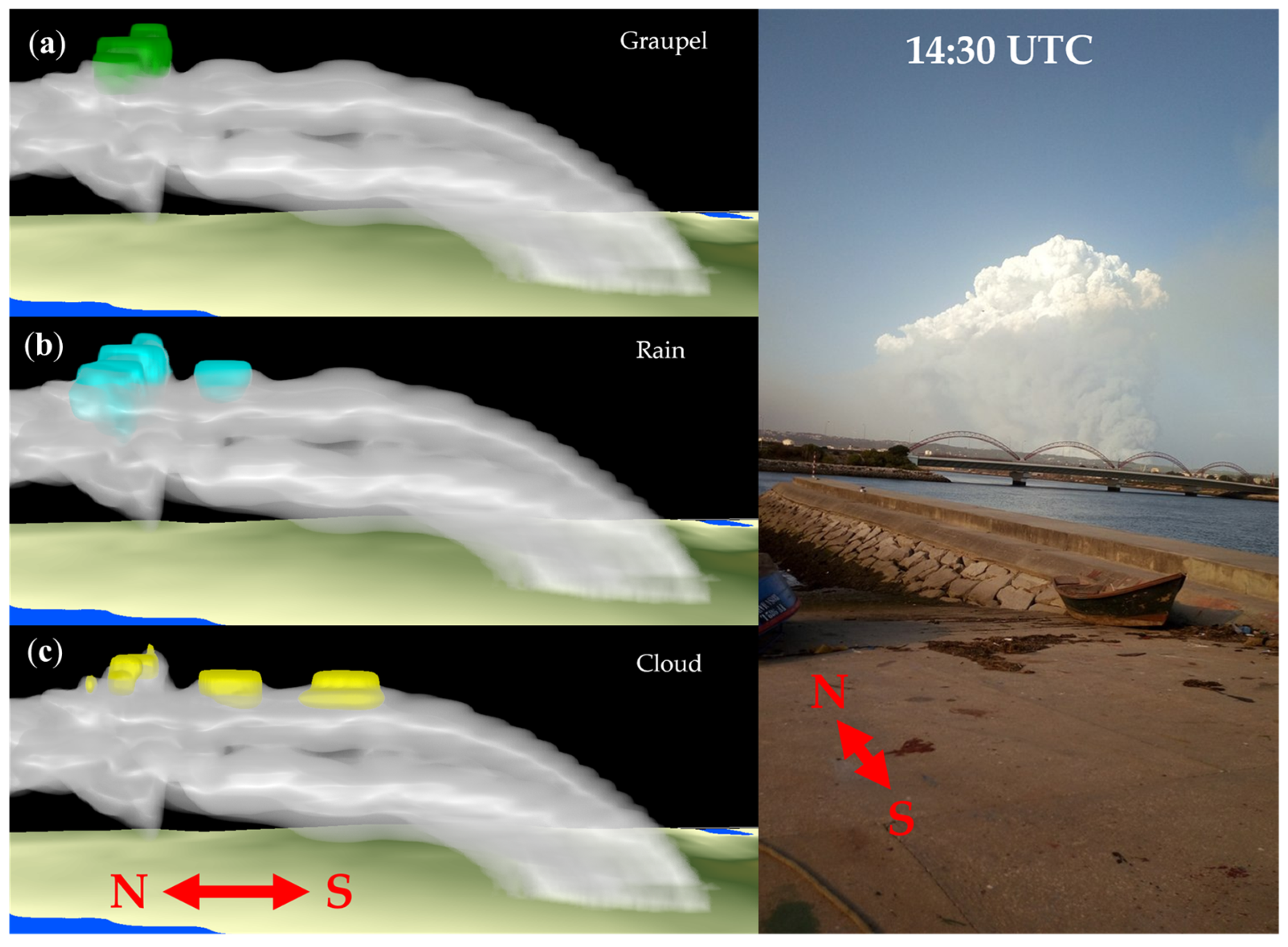
A comparison visualisation between the photographic evidence and the hydrometeors is shown in the Appendix A, Figure A6, where the presence of graupel, rainwater, and cloud water is observed in green, blue, and yellow, respectively, at 14:30 UTC. In this situation, cloud and rain water are present closer to the fire’s updraught, while graupel only forms further downstream. The configuration of the smoke plume and visible pyCu, shown in Appendix A, Figure A6, in the left and right panels, show that WRF-SFIRE was able to simulate hydrometeor formation at concurrent times with a similar plume geometry.
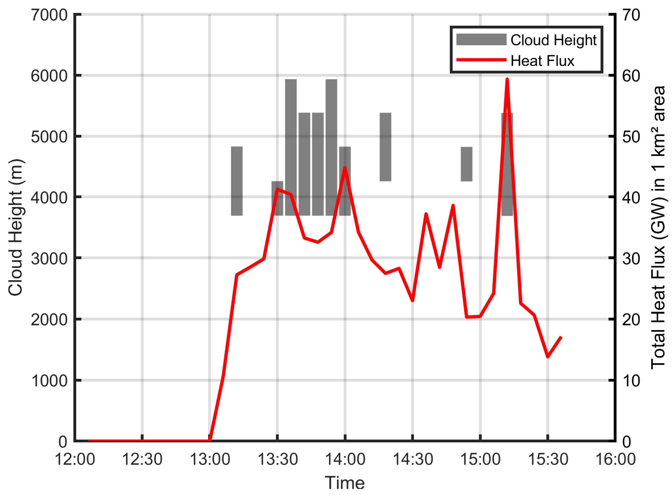
3.5.5. Fire Heat Fluxes Effect on Pyroconvective Cloud Formation
Figure 18 illustrates the effect of the surface heat fluxes from the fire into cloud formation. Heat flux values were taken along a 1 km × 1 km squared area centred on the fire head. Between 13 and 14 UTC, the formation of a ~2 km thick cloud is observed, lasting for roughly 30 min above 3750 m. Some individual clouds are shown to be temporally scattered, associated with heat flux values of above 30 GW during the initial hour of the wildfire. Between 14:30 and 14:50, heat flux once again overcomes the 30 GW threshold, producing a very shallow, roughly 0.5 km thick cloud, based at 4250 m and with a low vertical extension, preceding another brief formation of a 1.5 km deep cloud during a 60 GW peak of heat flux, based at 3750 m. This analysis shows that the conditions were initially more conductive to the formation of pyroconvection, as observed in [39], but began to deteriorate later into the afternoon. Moreover, the dependence on a continuous heat flux from the fire is highlighted, as once the energy supply is cut off, any clouds present quickly dissipate, coinciding with the overshooting pyroconvection profile [12].
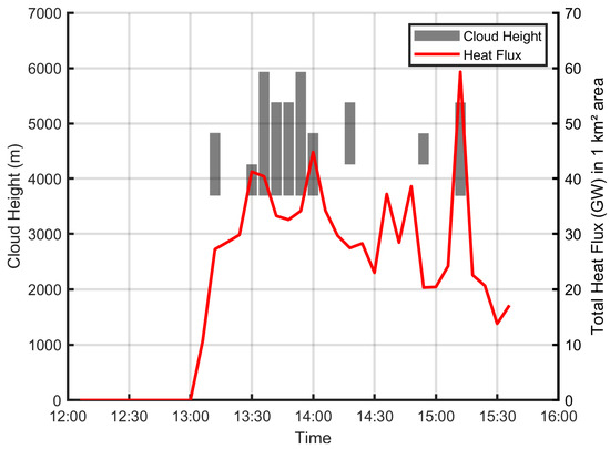
Figure 18.
Shaded grey bars denote the vertical extension of clouds present near the head of the fire and their height, on the left axis. In red, on right axis, the 1 km × 1 km total heat flux taken at the head of the fire is shown in GW.
3.6. Impacts of Simulation Setup on Potential Fire Spread
During the development of a simulation domain and physical parametrisation setup that would best represent the tropical cyclone’s flow, issues with the timing of the afternoon wind shift occurred. These issues were presented by other authors who attempted to use WRF-SFIRE to reproduce the Quiaios wildfire [34]. In simulations with no imposed fire, a SW wind flow would drive the fire into an urbanised area, thus hampering its progression. The wind would shift from SE to SW, as the tropical cyclone moved towards NE offshore, and would have occurred as early as 12 UTC, instead of the observed 15 UTC in weather stations reports [38].
The initial configuration for the simulations relied on a large parent domain that could capture more of Ophelia’s development, consisting of a total of four nested domains that improved the grid resolution to 100 m. The early wind shift would cause an increase in the RH and temperature, which would render fire spread impossible. Several tests were then performed to improve the wind shift timing, namely, changing PBL parametrisations, altering domain size and time of initialization, adding nudging at different time steps, and altering the model integration time step. None of the tests provided any improvements to the original issue, apart from changing the integration time step. Initially, a grid resolution of 6 times in seconds (6 dx), mentioned in the user’s guide as the upper limit [37] was used, with no numerical errors in the logs. When the resolution was increased from 6 to 5 dx, the results showed that the wind shift timing was delayed by more than 1h. Therefore, another simulation was performed with the current configuration and a time step of 3 dx to solve the early wind shift problem.
While in the study the fire was imposed, accurately describing the local meteorology was necessary to analyse the effects of the wildfire on the atmosphere.
4. Conclusions
To recreate the Quiaios wildfire event on 15 October 2017, the coupled atmosphere–fire model was used. A nested domain simulation was performed to downscale the large-scale atmospheric conditions created by the Tropical Cyclone Ophelia. The simulations underestimated the central pressure and wind speed of the tropical cyclone, but provided a consistent representation of the vertical atmosphere and meteorological conditions over Portugal. Dry and hot advection from the southern flow governed in the low levels, and a moist mid-level layer brought in humidity needed in setting the “inverted v” profile observed in vertical soundings [38,60], favourable to downdraft events [17].
The simulated surface temperature, humidity, and wind direction in d02 showed consensus with the weather stations, with the exception of a general overprediction of wind speed. In d03 and d04-LES, temperature and humidity changes from the arriving wind were poorly represented in the available stations, namely in d04-LES, where the temperature began decreasing much earlier than in the observations. Nonetheless, Figueira da Foz station was the only station available within the d04-LES implementation area, and was located near an elevation. In the remaining domain, the temperature drops occurred much later (Figure 9b). An LLJ was observed at approximately 15:00 UTC in vertical soundings and was well represented in d04-LES.
The fire was dominated by a two-layered plume, one underneath the PBL top (~2 km), and another that rose above the LCL, generating high-based convection, above 3.5 km height, with a low vertical extent (~2 km max.), which is characteristic of an overshooting type of proconvention, occurring when the LCL height is greater than the PBL [12]. The fire circulation generated indrafts that converged over the fireline and were carried upwards by the updraft, followed by a return flow that formed two vortex-like structures on the vertical plane. The descending branches of the fire circulation pushed the LLJ further, closer to the surface, thereby potentiating the wind speeds. A small-scale version of this upward and downward movement on the surface was observed prior to the fire, when the surface was populated by horizontal convective rolls, oriented with the wind and producing higher wind speed in the downwards branch of its shallow circulation. Most convective activity was governed by the fire-generated updraft because there was no CAPE that would provide parcel buoyancy. Sensible heat released from the fire was the main driver of the updrafts, carrying moisture of up to 4.8 g kg−1 to the LCL where it condensed. Despite the high intensity of the fire on the surface, the tilting of the updraft, displaced to the north-northeast, diluted most of the buoyancy from the plume, resulting in negative buoyancy as it reached the LCL. The latent heat released from condensation was not sufficient to overcome this difference in the temperature above the LCL; thus, any PyCu that formed very rapidly began dissipating, generating an area of negative vertical wind speeds downstream (Figure 13a). Moreover, a θe inversion zone 1.5 km above the LCL may have also contributed to keep the top of the plume from further growth. Due to this, no updrafts were registered inside any of the shallow PyCu. The composition of the shallow PyCu was mostly cloud water, with some rainwater appearing associated with downdrafts, likely from evaporative cooling of already negatively buoyant air. Ice, graupel, and snow mixing ratios were between five and seven times lesser than the cloud water mixing ratio, and their formation occurred at a delay from the PyCu appearance, above the freezing level. Furthermore, the fire contributed to moisture release on the order of 1.5–2 mm of PW within the fire plume.
No conclusions can be drawn in terms of fire feedback on the rate of spread, as the fire was prescribed to provide a better representation of the processes of the atmosphere–fire interactions, but additional information was given on the formation of PyCu associated with the Quiaios wildfire. WRF-SFIRE does not provide any information regarding the smoke plume interaction with the atmosphere, which has been shown to affect the dynamics of cloud formation and composition, when compared to regular convective clouds [11,14]. However, it does shed some light on a very rare event, during which the circulation of a Tropical Cyclone is directly related to extreme wildfire events. A sensitivity analysis to the model integration time-step could also provide further insights on how to more accurately simulate extreme weather events, improving the timing of how the model resolves large-scale weather (i.e., tropical cyclones), as referred to in §3.6. There is little information regarding time step validation in WRF simulations, but a lower time step has been shown to increase precipitation, hydrometeor condensation distribution, and microphysical processes [66]
Future applications of this research could improve the current understanding of atmospheric-fire circulation, providing information that could help firefighters by providing them with real-time terrain information, which would allow them to predict the conditions that could lead to the formation of either periodic or sustained pyroconvection and downburst potential. To that end, more accurate fuel information and fire spread validation are required in order to produce more accurate results, without the need to use of time of arrival data, together with the creation of new methods of assessing stability of the atmosphere under a wildfire. Nonethless, WRF-SFIRE was able to recreate pyroconvection via moisture and heat fluxes produced by the Quiaios wildfire, capturing its inherent plume dynamics and interaction with environmental wind.
Author Contributions
Conceptualization, investigation, software, data curation, validation, visualization, writing-original draft preparation, R.V.; methodology, formal analysis, writing-review and editing, R.S. and S.C.P.; methodology, formal analysis, writing-review and editing, supervision, A.C.C. and A.R.; formal analysis, writing-review and editing, project administration, funding acquisition, D.C. All authors have read and agreed to the published version of the manuscript.
Funding
Funding for this work was provided by the FCT—Fundação para a Ciência e a Tecnologia (Portuguese Foundation for Science and Technology) within the project ClimACT with the reference 2022.01896.PTDC and DOI 10.54499/2022.01896.PTDC (https://doi.org/10.54499/2022.01896.PTDC).
Data Availability Statement
The original contributions presented in this study are included in the article. Further inquiries can be directed to the corresponding author.
Acknowledgments
The authors acknowledge FCT for the financial support to UID Centro de Estudos do Ambiente e Mar (CESAM) + LA/P/0094/2020. David Carvalho acknowledges the FCT and the Ministry of Science, Technology and Higher Education (MCTES) for his researcher contract with the reference CEECINST/00013/2021/CP2779/CT0017 and DOI 10.54499/CEECINST/00013/2021/CP2779/CT0017 (https://doi.org/10.54499/CEECINST/00013/2021/CP2779/CT0017). Ricardo Vaz acknowledges the FCT/MCTES for the financial support for his PhD fellowship (PTDC/EME-REN/3460/2021). Rui Silva acknowledges the FCT for his PhD Grant (SFRH/BD/139020/2018). Susana Cardoso Pereira is a working member of COST Action CA 18135—FireLINKS (WG Member CA18135—Fire dynamics and prevention).
Conflicts of Interest
The authors declare no conflict of interest.
Appendix A
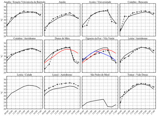
Figure A1.
Weather station observed 2 m temperature. (−+)—observation; bold black—d02; red—d03; blue—d04-LES.
Figure A1.
Weather station observed 2 m temperature. (−+)—observation; bold black—d02; red—d03; blue—d04-LES.
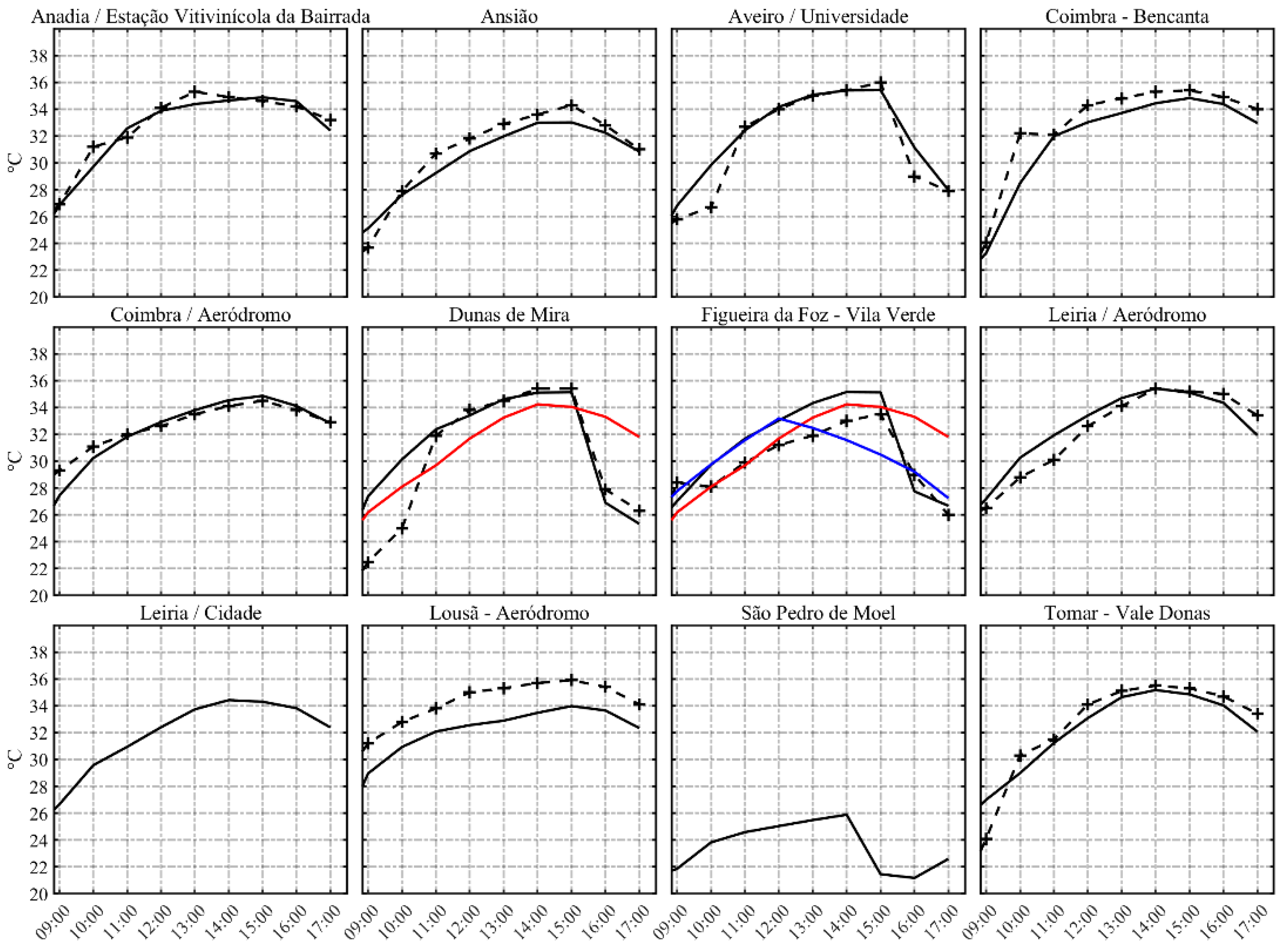
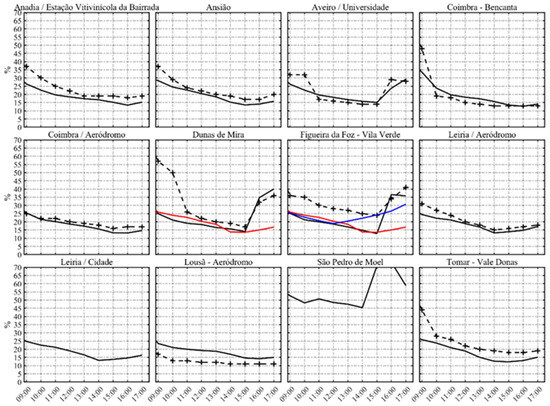
Figure A2.
Weather station observed 2 m RH. (−+)—observation; bold black—d02; red—d03; blue—d04-LES.
Figure A2.
Weather station observed 2 m RH. (−+)—observation; bold black—d02; red—d03; blue—d04-LES.
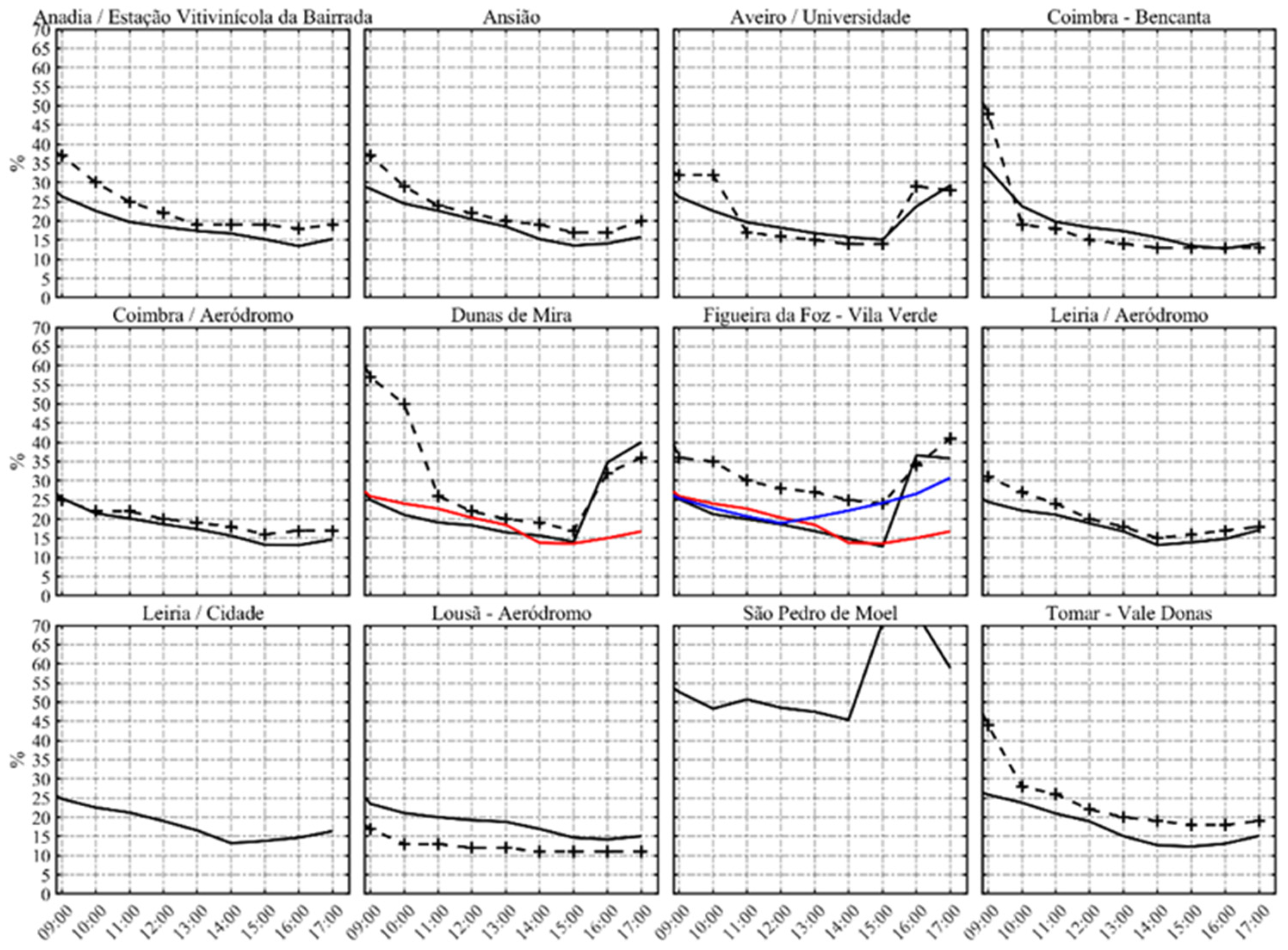

Figure A3.
Weather station observed 10 m wind speed. (−+)—observation; bold black—d02; red—d03; blue—d04-LES.
Figure A3.
Weather station observed 10 m wind speed. (−+)—observation; bold black—d02; red—d03; blue—d04-LES.
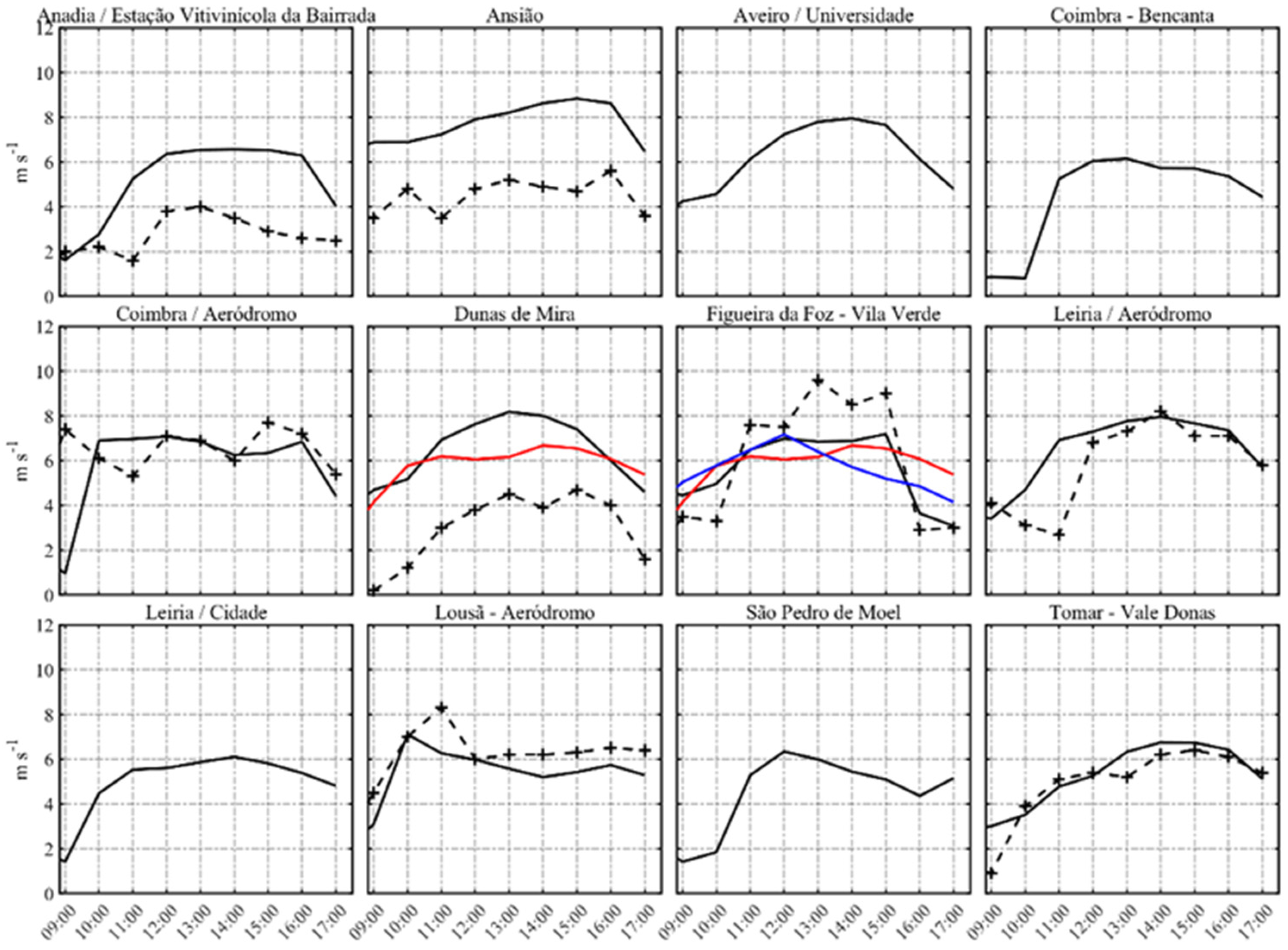
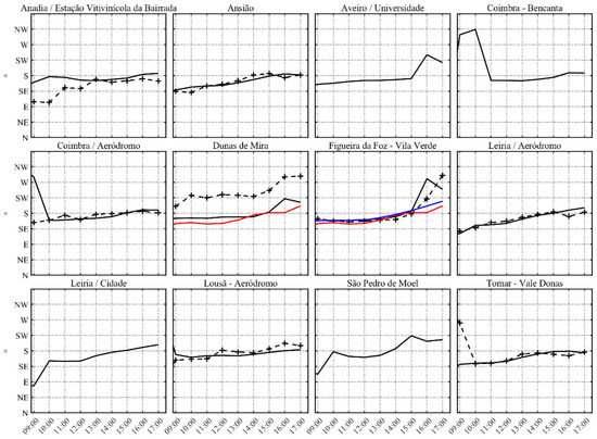
Figure A4.
Weather station observed 10 m wind direction. (−+)—observation; bold black—d02; red—d03; blue—d04-LES.
Figure A4.
Weather station observed 10 m wind direction. (−+)—observation; bold black—d02; red—d03; blue—d04-LES.
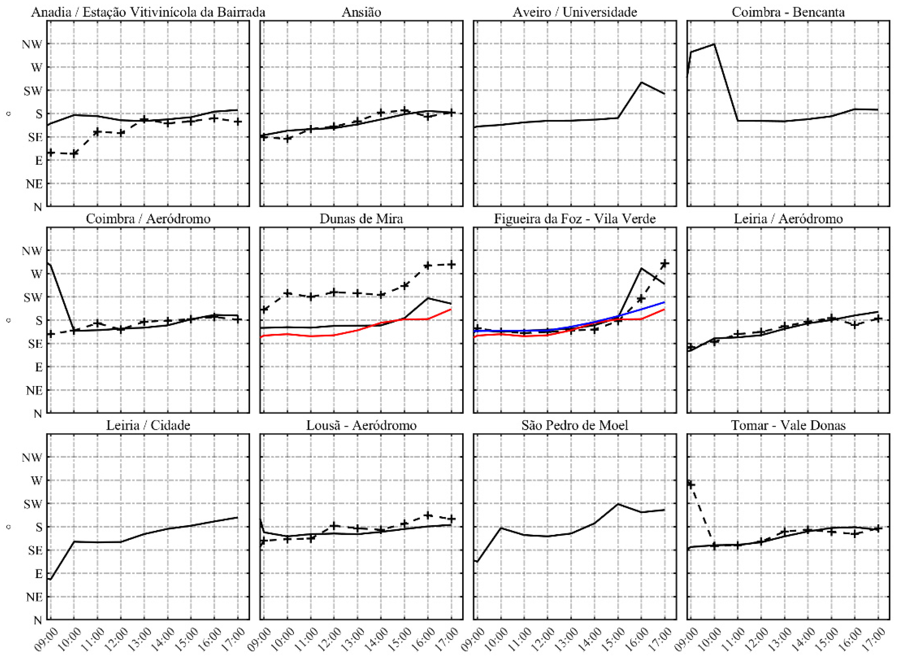
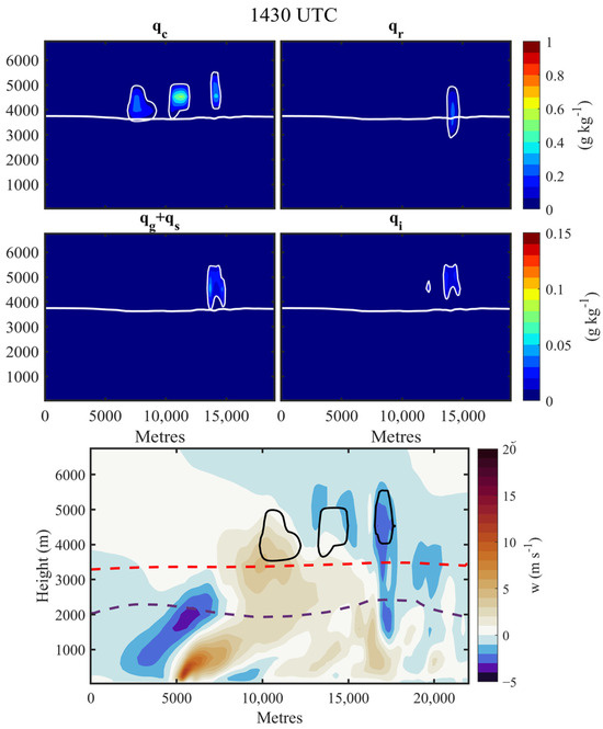
Figure A5.
Above: top left—cloud water mixing ratio (qc); top right—rainwater mixing ratio (qr); bottom left: snow and graupel mixing ratios (qg + qs); bottom right—ice mixing ratio (qi). The freezing level (T = 0 °C) is displayed in bold white. Below: vertical wind speed is shaded, dashed red line show the LCL height and dashed purple the PBL height.


Figure A6.
On the left panels, a VAPOR 3D visualisation of the fire plume and pyroconvection, shown in white tones and coloured tones, respectively. From top to bottom left the presence of graupel (a, green), rain (b, blue), and cloud (c, yellow) hydrometeors are displayed. On the right is a photography taken at 14:30 UTC from the coordinate point 40.1320 N, −8.8539 W [33,39]. The red arrows denote the orientation of the pictures.
References
- American Meteorological Society. Pyrocumulus. In Glossary of Meteorology. 2024. Available online: https://glossary.ametsoc.org/wiki/Pyrocumulus (accessed on 26 March 2025).
- American Meteorological Society. Pyrocumulonimbus. In Glossary of Meteorology. 2024. Available online: https://glossary.ametsoc.org/wiki/Pyrocumulonimbus (accessed on 26 March 2025).
- Potter, B.E. Atmospheric Interactions with Wildland Fire Behaviour—I. Basic Surface Interactions, Vertical Profiles and Synoptic Structures. Int. J. Wildland Fire 2012, 21, 779. [Google Scholar] [CrossRef]
- Allen, C.D.; Macalady, A.K.; Chenchouni, H.; Bachelet, D.; McDowell, N.; Vennetier, M.; Kitzberger, T.; Rigling, A.; Breshears, D.D.; Hogg, E.H.; et al. A Global Overview of Drought and Heat-Induced Tree Mortality Reveals Emerging Climate Change Risks for Forests. For. Ecol. Manag. 2010, 259, 660–684. [Google Scholar] [CrossRef]
- Bugmann, H.; Palahi, M.; Bontemps, H.D.; Tome, M. Trends in Modeling to Address Forest Management and Environmental Challenges in Europe: Introduction. For. Syst. 2010, 19, 3–7. [Google Scholar] [CrossRef]
- Moritz, M.A.; Morais, M.E.; Summerell, L.A.; Carlson, J.M.; Doyle, J. Wildfires, Complexity, and Highly Optimized Tolerance. Proc. Natl. Acad. Sci. USA 2005, 102, 17912–17917. [Google Scholar] [CrossRef] [PubMed]
- Senande-Rivera, M.; Insua-Costa, D.; Miguez-Macho, G. Spatial and Temporal Expansion of Global Wildland Fire Activity in Response to Climate Change. Nat. Commun. 2022, 13, 1208. [Google Scholar] [CrossRef] [PubMed]
- Luderer, G.; Trentmann, J.; Andreae, M.O. A New Look at the Role of Fire-Released Moisture on the Dynamics of Atmospheric Pyro-Convection. Int. J. Wildland Fire 2009, 18, 554. [Google Scholar] [CrossRef]
- Tory, K.J.; Thurston, W.; Kepert, J.D. Thermodynamics of Pyrocumulus: A Conceptual Study. Mon. Weather Rev. 2018, 146, 2579–2598. [Google Scholar] [CrossRef]
- Potter, B.E. The Role of Released Moisture in the Atmospheric Dynamics Associated with Wildland Fires. Int. J. Wildland Fire 2005, 14, 77. [Google Scholar] [CrossRef]
- Fromm, M.; Lindsey, D.T.; Servranckx, R.; Yue, G.; Trickl, T.; Sica, R.; Doucet, P.; Godin-Beekmann, S. The Untold Story of Pyrocumulonimbus. Bull. Amer. Meteor. Soc. 2010, 91, 1193–1210. [Google Scholar] [CrossRef]
- Castellnou, M.; Bachfischer, M.; Miralles, M.; Ruiz, B.; Stoof, C.R.; Vilà-Guerau De Arellano, J. Pyroconvection Classification Based on Atmospheric Vertical Profiling Correlation With Extreme Fire Spread Observations. JGR Atmos. 2022, 127, e2022JD036920. [Google Scholar] [CrossRef]
- Luderer, G.; Trentmann, J.; Winterrath, T.; Textor, C.; Herzog, M.; Graf, H.F.; Andreae, M.O. Modeling of Biomass Smoke Injection into the Lower Stratosphere by a Large Forest Fire (Part II): Sensitivity Studies. Atmos. Chem. Phys. 2006, 6, 5261–5277. [Google Scholar] [CrossRef]
- Peterson, D.A.; Hyer, E.J.; Campbell, J.R.; Solbrig, J.E.; Fromm, M.D. A Conceptual Model for Development of Intense Pyrocumulonimbus in Western North America. Mon. Weather Rev. 2017, 145, 2235–2255. [Google Scholar] [CrossRef]
- Thurston, W.; Tory, K.J.; Fawcett, R.; Kepert, J.D. Large-Eddy Simulations of Pyro-Convection and Its Sensitivity to Environmental Conditions. In Proceedings of the Research Proceedings, Bushfire and Natural Hazards CRC & AFAC 2015 Conference’, Bushfire and Natural Hazards CRC, Adelaide, Australia, 1–3 September 2015; pp. 148–160. [Google Scholar]
- Tory, K.; Thurston, W. Pyrocumulonimbus: A Literature Review; Bushfire and Natural Hazards CRC: East Melbourne, Australia, 2015. [Google Scholar]
- Wakimoto, R.M. Forecasting Dry Microburst Activity over the High Plains. Mon. Wea. Rev. 1985, 113, 1131–1143. [Google Scholar] [CrossRef]
- Tory, K.J.; Kepert, J.D. Pyrocumulonimbus Firepower Threshold: Assessing the Atmospheric Potential for pyroCb. Weather Forecast. 2021, 36, 439–456. [Google Scholar] [CrossRef]
- Bakhshaii, A.; Johnson, E.A. A Review of a New Generation of Wildfire–Atmosphere Modeling. Can. J. For. Res. 2019, 49, 565–574. [Google Scholar] [CrossRef]
- Peace, M.; Greenslade, J.; Ye, H.; Kepert, J.D. Simulations of the Waroona Fire Using the Coupled Atmosphere–Fire Model ACCESS-Fire. J. South. Hemisph. Earth Syst. Sci. 2022, 72, 126–138. [Google Scholar] [CrossRef]
- Trentmann, J.; Luderer, G.; Winterrath, T.; Fromm, M.D.; Servranckx, R.; Textor, C.; Herzog, M.; Graf, H.-F.; Andreae, M.O. Modeling of Biomass Smoke Injection into the Lower Stratosphere by a Large Forest Fire (Part I): Reference Simulation. Atmos. Chem. Phys. 2006, 6, 5247–5260. [Google Scholar] [CrossRef]
- Kochanski, A.K.; Jenkins, M.A.; Yedinak, K.; Mandel, J.; Beezley, J.; Lamb, B. Toward an Integrated System for Fire, Smoke and Air Quality Simulations. Int. J. Wildland Fire 2016, 25, 534. [Google Scholar] [CrossRef]
- San-Miguel-Ayanz, J.; Durrant, T.; Boca, R.; Maianti, P.; Libertà, G.; Artés Vivancos, T.; Oom, D.; Branco, A.; Tomàs Rigo, D.; Ferrari, D.; et al. Forest Fires in Europe, Middle East and North Africa 2020; Publications Office of the European Union: Luxembourg, 2021; ISBN 978-92-76-42351-5. [Google Scholar]
- Hoinka, K.P.; Carvalho, A.; Miranda, A.I. Regional-Scale Weather Patterns and Wildland Fires in Central Portugal. Int. J. Wildland Fire 2009, 18, 36. [Google Scholar] [CrossRef]
- Parente, J.; Pereira, M.G.; Amraoui, M.; Fischer, E.M. Heat Waves in Portugal: Current Regime, Changes in Future Climate and Impacts on Extreme Wildfires. Sci. Total Environ. 2018, 631–632, 534–549. [Google Scholar] [CrossRef]
- Ermitão, T.; Páscoa, P.; Trigo, I.; Alonso, C.; Gouveia, C. Mapping the Most Susceptible Regions to Fire in Portugal. Fire 2023, 6, 254. [Google Scholar] [CrossRef]
- Aparício, B.A.; Alcasena, F.; Ager, A.; Chung, W.; Pereira, J.M.C.; Sá, A.C.L. Evaluating Priority Locations and Potential Benefits for Building a Nation-Wide Fuel Break Network in Portugal. J. Environ. Manag. 2022, 320, 115920. [Google Scholar] [CrossRef]
- 8.o Relatório Provisório De Incêndios Rurais 2024; Direção Nacional de Gestão do Programa de Fogos Rurais: Lisbon, Portugal, 2024; p. 14.
- Guerreiro, J.; Fonseca, C.; Salgueiro, A.; Fernandes, P.; Lopez, E.; de Neufville, R.; Mateus, F.; Castellnou, M.; Silva, J.S.; Moura, J.; et al. Análise e Apuramento Dos Factos Relativos Aos Incêndios Que Ocorreram Em Pedrogão Grande. In Castanheira De Pera Ansião Alvaiázere Figueiró Dos Vinhos Arganil Góis Penela Pampilhosa Da Serra Oleiros E Sertã Entre; Assembleia da República: Lisbon, Portugal, 2017; Volume 17. [Google Scholar]
- Ramos, A.M.; Russo, A.; DaCamara, C.C.; Nunes, S.; Sousa, P.; Soares, P.M.M.; Lima, M.M.; Hurduc, A.; Trigo, R.M. The Compound Event That Triggered the Destructive Fires of October 2017 in Portugal. iScience 2023, 26, 106141. [Google Scholar] [CrossRef]
- Viegas, D.X.; Almeida, M.F.; Ribeiro, L.M.; Raposo, J.; Viegas, M.T.; Oliveira, R.; Alves, D.; Pinto, C.; Rodrigues, A.; Ribeiro, C.; et al. Análise Dos Incêndios Florestais Ocorridos a 15 de Outubro de 2017; Centro de Estudos sobre Incêndios Florestais (CEIF/ADAI/LAETA): Coimbra, Portugal, 2019. [Google Scholar]
- Castellnou, M.; Guiomar, N.; Rego, F.; Fernandes, P.M. Fire growth patterns in the 2017 mega fire episode of October 15, central Portugal. In Advances in Forest Fire Research 2018; Imprensa da Universidade de Coimbra: Coimbra, Portugal, 2018; pp. 447–453. ISBN 978-989-26-1650-6. [Google Scholar]
- Campos, C.; Couto, F.T.; Filippi, J.-B.; Baggio, R.; Salgado, R. Modelling Pyro-Convection Phenomenon during a Mega-Fire Event in Portugal. Atmos. Res. 2023, 290, 106776. [Google Scholar] [CrossRef]
- Couto, F.; Salgado, R.; Filippi, J.-B.; Baggio, R.; Kartsios, S.; Cardoso, R.; Soares, P.; Campos, C. Intercomparação de Simulações Numéricas Com Modelos Atmosféricos Acoplados a Modelos de Propagação de Fogo. Rep. I 2023, 1, 1. [Google Scholar]
- Mandel, J.; Amram, S.; Beezley, J.D.; Kelman, G.; Kochanski, A.K.; Kondratenko, V.Y.; Lynn, B.H.; Regev, B.; Vejmelka, M. Recent Advances and Applications of WRF–SFIRE. Nat. Hazards Earth Syst. Sci. 2014, 14, 2829–2845. [Google Scholar] [CrossRef]
- Mandel, J.; Beezley, J.D.; Kochanski, A.K. Coupled Atmosphere-Wildland Fire Modeling with WRF 3.3 and SFIRE 2011. Geosci. Model Dev. 2011, 4, 591–610. [Google Scholar] [CrossRef]
- Skamarock, W.C.; Klemp, J.B.; Dudhia, J.; Gill, D.O.; Liu, Z.; Berner, J.; Wang, W.; Powers, J.G.; Duda, M.G.; Barker, D.M.; et al. A Description of the Advanced Research WRF Model Version 4; UCAR/NCAR: Boulder, CO, USA, 2019. [Google Scholar]
- Simões, I.; Pinto, P.; Silva, Á.; Pereira, M.; Barroso, C.; Santos, M.; Lopes, M.; Moreira, N.; Correira, S. Os Incêndios Florestais de 14 a 16 de Outubro de 2017 Em Portugal Continental; IPMA: Albany, NY, USA, 2018. [Google Scholar]
- Fozaominuto, Incêndios No Concelho Da Figueira Da Foz: Quiaios e Paião. Available online: https://www.fozaominuto.com/2017/10/incendios-no-concelho-da-figueira-da_15.html (accessed on 26 March 2025).
- Osher, S.; Fedkiw, R.P. Level Set Methods and Dynamic Implicit Surfaces; Springer: New York, NY, USA, 2003; ISBN 978-0-387-22746-7. [Google Scholar]
- Rothermel, R.C. A Mathematical Model for Predicting Fire Spread in Wildland Fuels; Intermountain Forest & Range Experiment Station, Forest Service, US Department of Agriculture: Ogden, UT, USA, 1972; Volume 115.
- Albini, F.A. Estimating Wildfire Behavior and Effects; Department of Agriculture, Forest Service, Intermountain Forest and Range Experiment Station: Ogden, UT, USA, 1976; Volume 30.
- Anderson, H. Aids to Determining Fuel Models for Estimating Fire Behavior. General Technical Report INT-122; US Department of Agriculture Forest Service, Intermountain Forest and Range Experiment Station: Ogden, UT, USA, 1982.
- Hersbach, H.; Bell, B.; Berrisford, P.; Hirahara, S.; Horányi, A.; Muñoz-Sabater, J.; Nicolas, J.; Peubey, C.; Radu, R.; Schepers, D.; et al. The ERA5 Global Reanalysis. Quart J. R. Meteoro Soc. 2020, 146, 1999–2049. [Google Scholar] [CrossRef]
- Hong, S.-Y. Hongandlim-JKMS-2006. J. Korean Meteorol. Soc. 2006, 42, 129. [Google Scholar]
- Kain, J.S. The Kain–Fritsch Convective Parameterization: An Update. J. Appl. Meteor. 2004, 43, 170–181. [Google Scholar] [CrossRef]
- Iacono, M.J.; Delamere, J.S.; Mlawer, E.J.; Shephard, M.W.; Clough, S.A.; Collins, W.D. Radiative Forcing by Long-lived Greenhouse Gases: Calculations with the AER Radiative Transfer Models. J. Geophys. Res. 2008, 113, 2008JD009944. [Google Scholar] [CrossRef]
- Hong, S.-Y.; Noh, Y.; Dudhia, J. A New Vertical Diffusion Package with an Explicit Treatment of Entrainment Processes. Mon. Weather Rev. 2006, 134, 2318–2341. [Google Scholar] [CrossRef]
- Niu, G.-Y.; Yang, Z.-L.; Mitchell, K.E.; Chen, F.; Ek, M.B.; Barlage, M.; Kumar, A.; Manning, K.; Niyogi, D.; Rosero, E.; et al. The Community Noah Land Surface Model with Multiparameterization Options (Noah-MP): 1. Model Description and Evaluation with Local-Scale Measurements. J. Geophys. Res. 2011, 116, D12109. [Google Scholar] [CrossRef]
- Yang, Z.-L.; Niu, G.-Y.; Mitchell, K.E.; Chen, F.; Ek, M.B.; Barlage, M.; Longuevergne, L.; Manning, K.; Niyogi, D.; Tewari, M.; et al. The Community Noah Land Surface Model with Multiparameterization Options (Noah-MP): 2. Evaluation over Global River Basins. J. Geophys. Res. 2011, 116, D12110. [Google Scholar] [CrossRef]
- De Meij, A.; Vinuesa, J.F. Impact of SRTM and Corine Land Cover Data on Meteorological Parameters Using WRF. Atmos. Res. 2014, 143, 351–370. [Google Scholar] [CrossRef]
- Jee, J.-B.; Kim, S. Sensitivity Study on High-Resolution Numerical Modeling of Static Topographic Data. Atmosphere 2016, 7, 86. [Google Scholar] [CrossRef]
- Jiménez-Esteve, B.; Udina, M.; Soler, M.R.; Pepin, N.; Miró, J.R. Land Use and Topography Influence in a Complex Terrain Area: A High Resolution Mesoscale Modelling Study over the Eastern Pyrenees Using the WRF Model. Atmos. Res. 2018, 202, 49–62. [Google Scholar] [CrossRef]
- OpenTopography, Shuttle Radar Topography Mission (SRTM) Global. 2013. Available online: https://opentopography.org/meta/OT.042013.4326.1 (accessed on 26 March 2025).
- European Environment Agency. CORINE Land Cover 2012 (Raster 100 m), Europe, 6-Yearly—Version 2020_20u1. May 2020. Available online: https://sdi.eea.europa.eu/catalogue/copernicus/api/records/a84ae124-c5c5-4577-8e10-511bfe55cc0d?language=all (accessed on 26 March 2025).
- Pineda, N.; Jorba, O.; Jorge, J.; Baldasano, J.M. Using NOAA AVHRR and SPOT VGT Data to Estimate Surface Parameters: Application to a Mesoscale Meteorological Model. Int. J. Remote Sens. 2004, 25, 129–143. [Google Scholar] [CrossRef]
- Copernicus Land Monitoring Service EU-DEM v1.1 2016. Available online: https://land.copernicus.eu/imagery-in-situ/eu-dem (accessed on 26 March 2025).
- Benali, A.; Guiomar, N.; Gonçalves, H.; Mota, B.; Silva, F.; Fernandes, P.M.; Mota, C.; Penha, A.; Santos, J.; Pereira, J.M.C.; et al. The Portuguese Large Wildfire Spread Database (PT-FireSprd). Earth Syst. Sci. Data 2023, 15, 3791–3818. [Google Scholar] [CrossRef]
- Copernicus Climate Change Service. In Situ Observations of Meteorological Variables from the Integrated Global Radiosounding Archive and the Radiosounding Harmonization Dataset from 1978 Onward. 2021. Available online: https://cds.climate.copernicus.eu/datasets/insitu-observations-igra-baseline-network?tab=overview (accessed on 26 March 2025).
- Brown, D.; Brownrigg, R.; Haley, M.; Huang, W. NCAR Command Language (NCL). 2012. Available online: https://www.unidata.ucar.edu/software/netcdf/workshops/2012/third_party/NCL.html (accessed on 26 March 2025).
- Zhang, Y.; Gao, Z.; Li, D.; Li, Y.; Zhang, N.; Zhao, X.; Chen, J. On the Computation of Planetary Boundary-Layer Height Using the Bulk Richardson Number Method. Geosci. Model Dev. 2014, 7, 2599–2611. [Google Scholar] [CrossRef]
- Stewart, S. National Hurricane Center Tropical Cyclone Report: Hurricane Ophelia (AL172017); Tech. rep.; NOAA: National Hurrican Center: Miami, FL, USA, 2018.
- Stull, R.B. Mean Boundary Layer Characteristics. In An Introduction to Boundary Layer Meteorology; Springer: Berlin/Heidelberg, Germany, 1988; pp. 1–27. [Google Scholar]
- Carvalho, D.; Rocha, A.; Gómez-Gesteira, M.; Santos, C. A Sensitivity Study of the WRF Model in Wind Simulation for an Area of High Wind Energy. Environ. Model. Softw. 2012, 33, 23–34. [Google Scholar] [CrossRef]
- Potter, B.E. A Dynamics Based View of Atmosphere—Fire Interactions. Int. J. Wildland Fire 2002, 11, 247. [Google Scholar] [CrossRef]
- Barrett, A.I.; Wellmann, C.; Seifert, A.; Hoose, C.; Vogel, B.; Kunz, M. One Step at a Time: How Model Time Step Significantly Affects Convection-Permitting Simulations. J. Adv. Model Earth Syst. 2019, 11, 641–658. [Google Scholar] [CrossRef]

Disclaimer/Publisher’s Note: The statements, opinions and data contained in all publications are solely those of the individual author(s) and contributor(s) and not of MDPI and/or the editor(s). MDPI and/or the editor(s) disclaim responsibility for any injury to people or property resulting from any ideas, methods, instructions or products referred to in the content. |
© 2025 by the authors. Licensee MDPI, Basel, Switzerland. This article is an open access article distributed under the terms and conditions of the Creative Commons Attribution (CC BY) license (https://creativecommons.org/licenses/by/4.0/).