Aspects Regarding the CO₂ Footprint Developed by Marine Diesel Engines

Abstract

This study examines the emissions generated by a tall ship of 81.36 m length under various operating conditions, focusing particularly on carbon dioxide emissions at different navigation speeds. The main purpose of the paper is to establish theoretical and practical methods for calculating and measuring the level of CO₂ emitted by the ship engines. Additionally, this article compares the results of carbon dioxide emission calculations based on theoretical methods with the results of real measurements. The paper verifies and assesses the carbon dioxide emission calculation methods compared to the emissions measured in real conditions for diesel engines. A comparative analysis of several methods for determining CO₂ emissions leads to much more accurate and conclusive results close to reality. The results obtained through empirical and theoretical methods for determining CO₂ emissions from the main engine demonstrate that the difference between these values is more accurate at lower engine loads but shows discrepancies at higher loads due to real-world inefficiencies, combustion variations, and model simplifications. The measured CO₂ emission values for auxiliary engines at 60% load demonstrate consistency and closely reflect real operating conditions, while analytical calculations tend to be higher due to theoretical losses and model assumptions. Stoichiometric values fall in between, assuming ideal combustion but lacking adjustments for real variables. This highlights the efficiency of the diesel generator and the importance of empirical data in capturing actual emissions more accurately. The investigation aims to provide a detailed understanding of CO₂ emission variations based on the ship’s operating parameters, including the study of these emissions at the level of the main diesel propulsion engine as well as the auxiliary engines. By analyzing these methods for determining engine emissions, conclusions can be reached about aspects such as the following: engine wear condition, efficiency losses, or incomplete combustion. This analysis has the potential to guide the implementation of new policies and technologies aimed at minimizing the carbon footprint of a reference ship, considering the importance of sustainable resource management and environmental protection in a viable long-term manner.

1. Introduction

To address the challenges of climate change, the international community has adopted a series of strategic and policy measures aimed at reducing GHG (greenhouse gas) emissions and promoting sustainable development. The most important initiatives include international agreements, global conferences, and regional policies [1].

The Paris Agreement, adopted in 2015 at the Conference of the Parties (COP 21) to the United Nations Framework Convention on Climate Change (UNFCCC), represents a turning point in the global efforts to combat climate change. The agreement aims to limit the increase in global temperature this century and remain significantly below 2 °C above pre-industrial levels, with the aim of keeping this increase around 1.5 °C. Each country that signed the Paris Agreement [2] has set its Nationally Determined Contributions (NDCs) to reduce GHG emissions.

COP28, held in 2023, continued the efforts initiated by the Paris Agreement, providing a forum for negotiations and discussions on new targets and measures to reduce emissions. Conferences of the Parties are annual events where participating countries present their progress and adjust their strategies to address emerging challenges. COP28 focused on implementing adaptation measures and supporting developing countries in their efforts to reduce emissions.

The European Union (EU) is an important leader in combating climate change, adopting an ambitious package of policies and measures to reduce GHG emissions. Among the EU’s most important initiatives is the European Green Deal [3], which aims to make Europe the first climate-neutral continent by 2050. This plan includes measures to promote renewable energy, energy efficiency, and sustainable mobility.

The EU Effort Sharing Regulation sets national emission reduction targets for sectors not covered by the Emissions Trading System (ETS). These targets are adjusted according to the economic capacity of each Member State, thus ensuring a fair transition to a low-carbon economy. The EU Hydrogen Strategy also promotes the use of green hydrogen as a solution for the decarbonization of the industrial and heavy transport sectors.

In addition to government initiatives, numerous international organizations, companies, and NGOs are contributing to global efforts to combat climate change. Reforestation projects, investments in green technologies, and public awareness campaigns [4] are just a few examples of concrete actions that complement the policies and measures adopted by governments.

In the current context of climate change and increasing environmental concerns, the analysis of emissions generated by the combustion of fossil fuels has become a topic of major importance. Emissions of pollutants, which include substances such as carbon dioxide (CO₂), nitrogen oxides (NOx), and unburned hydrocarbons (HC), are among the main causes of air pollution and have harmful effects on human health and ecosystems [3,5].

The main objectives of the paper are as follows:

1.

To establish theoretical and practical methods for calculating and measuring the level of CO₂ emitted by ship engines.

2.

To compare the results of CO₂ emission calculations based on theoretical methods with the results of real measurements.

3.

To verify and assess the CO₂ emission calculation methods compared to the emission measured in real conditions for diesel engines.

4.

To conduct a comparative analysis of several methods for determining CO₂ emissions, with the aim of obtaining much more accurate and conclusive results close to reality.

The scope of the research conducted is to analyze, both practically and theoretically, the CO₂ emissions generated by the diesel engines on board a sailing ship in different cruising modes. Sailing modes are understood as the various operating conditions of the engines in order to develop different cruising speeds of the ship. Each of these modes has distinct characteristics and influences differently the amount of CO₂ emitted.

2. Literature Review

Starting in 2008, the International Maritime Organization (IMO) adopted the Resolution MEPC.177(58) [6], which focuses on controlling NOx emissions from marine diesel engines and ensuring compliance with NOx emission limits.

With the limitations imposed by the IMO in 2011 [7], numerous researchers have focused their studies on establishing a calculation for determining the amount of CO₂ in engine exhaust gases that reflects the real value of emissions as much as possible. In this context, in 2016, Cosofret et al. [8] established a method for determining the mass emissions of CO₂ from the exhaust gases of marine diesel engines named the stoichiometric method based on the NOx technical code [9].

In 2020, IMO established an estimated calculation formula in the Fourth Greenhouse Gas Study 2020 [10] for the specific fuel consumption of main engines. Based on this formula, it is very easy to theoretically calculate the hourly consumption and the amount of CO₂ emitted.

Based on the previously presented references [6,7,8,9], a series of articles have been developed regarding theoretical calculations and measurements related to CO₂ emissions from engines. Thus, Rongbin Xin et al. [11], assuming the molecular formula of the fuel C_aH_bO_cN_dS_e, calculated the mass of CO₂ for the 6RT-flex58T-D, a large two-stroke low-speed marine diesel engine produced by Wartsila. In addition, Seunghun Lim et al. [12] developed a carbon balance method to calculate the exhaust flow rate using the concentration of carbon dioxide (CO₂), carbon monoxide (CO), and total hydrocarbon (THC) in exhaust gas and fuel consumption for slow-speed and high-speed ship engines. He performed measurements for five marine engines of different sizes and obtained values between 3144.43 and 3150.58 KgCO₂/ton of fuel, approximately 3.58 KgCO₂/Kg of fuel. To gain a clearer picture of CO₂ emissions from marine diesel engines, Lamia Salehin et al. [13] measured emissions from 12 Wartsila naval engines so that the study could be used as a benchmark for the field. The aim of the study was to create a more descriptive graph of CO₂ emissions from marine diesel engines. According to [13], emissions were measured for the Wartsila 6L20F engine with a power of 1200 kW, obtaining 0.709 tons of CO₂/h, approximately 0.59 KgCO₂/kWh. Researchers have also studied ways to reduce CO2 emissions using alternative fuels or mixtures of conventional and alternative fuels. Thus, Robert Madalin Chivu et al. [14] studied a way to reduce CO₂ emissions by mixing diesel fuel with eucalyptus oil in an HDI (high-pressure direct injection) engine. This led to decreases of up to 8% in CO₂ concentrations. In the article [15], Ivica Skoko et al. calculated CO₂ emissions for both a Wartsila 20 diesel engine and a hybrid system with a Caterpillar 3516C engine, comparing the values obtained. The conclusion was that it achieved results regarding a decrease in CO₂ emissions by approximately 18%. The present work aims to compile a series of theoretical methodologies, allowing their results to be compared with practical measurements.

By analyzing the emissions of the ship and the international IMO recommendations to reduce CO₂ emissions, this work can contribute to the awareness of decision-makers for the implementation of the energy efficiency management concept of ships. This approach aligns with environmental sustainability goals while enhancing operational performance in the maritime sector.

3. Materials and Methods of Research

The materials and methods will be based on the scopes of application of the research carried out, which are the following:

• Determining CO₂ emission mass flow rates: Establishing the mass flow rates of CO₂ emissions across various sailing regimes using direct measurements.
• Analytical evaluation of CO₂ emissions: Conducting analytical calculations to determine the CO₂ emission mass flow rates for ship diesel engines at different working loads.
• Stoichiometric evaluation of CO₂ emissions: Applying chemical equation to calculate the CO₂ emission mass flow rates for reference ship diesel engines at different working loads.
• Comparison of methodologies: Analyzing the methods for determining CO₂ emission mass flow rates by contrasting direct measurement results with the results obtained by the two methods: analytical and stoichiometric [16].

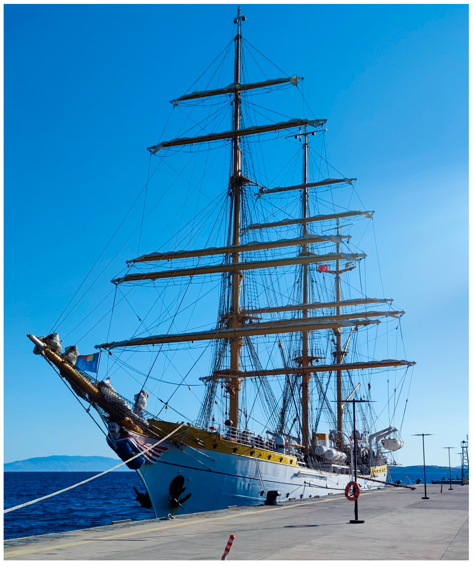
3.1. The Ship with Mechanical Equipment Onboard

The research was carried out on a sailing ship constructed for training cadet students. The training ship, shown in Figure 1, with general characteristics listed in

Table 1. General characteristics of the ship [17].

Characteristics	Value
Maximum length	81.36 [m]
Draft 1	5.35 [m]
Maximum speed	9.5 [knots]
Deadweight	1840 [tones]

¹ The draft of a ship refers to the vertical distance between the waterline and the bottom of the hull (the keel).

, is a class A sailing ship where propulsion is achieved using a classical diesel engine system. Additionally, the vessel can navigate using wind power, as it is equipped with 23 sails that add up to a total sail area of 1850 m². This feature enables it to operate as a hybrid system, combining diesel engine propulsion with wind-powered sailing, enhancing its versatility and energy efficiency. The ship’s mechanical propulsion system is a classic type with a single shaft line and comprises a four-stroke MAK main engine, a gearbox, a shaft line, and a controllable pitch propeller. In addition, the ship is also equipped with 3 MAN diesel generators for producing electricity on board.

The ship classic propulsion system chin includes the following:

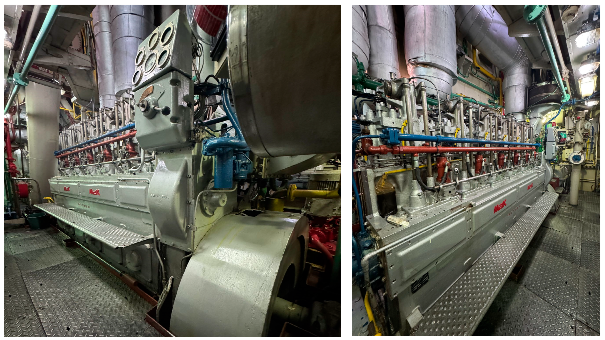
• Main Engine—MAK 6 MU 451 main engine, providing the necessary power for the ship’s movement.
• Reducer (Gearbox)—Reduces the engine’s speed to an optimal level for the propeller. In this case, the speed is reduced from (main engine) 375 rpm to (propeller and shaft line) 250 rpm.
• Propeller Shaft—The shaft that transmits rotational motion from the gearbox to the propeller.
• Controllable-Pitch Propeller (CPP)—This type of propeller allows adjustment of the blade angles, optimizing propulsion efficiency based on navigation conditions and power requirements.

The MAK 6 MU 451 main engine, shown in Figure 2, is produced by the MAK company and is known for marine and industrial use. This engine is recognized for its reliability, efficiency, and durability. The MAK 6 MU 451 engine, with its specifications presented in

Table 2. General characteristics of the MAK 6 MU 451 main diesel engine.

Characteristics	Value
Engine type	4-stroke, diesel
Engine power	810 [kW]
Speed	375 [rpm]
Fuel type	Marine diesel oil
Specific fuel consumption	215 [g/kWh]
Year of manufacture	1969
Year of last major overhaul	2020

, is a four-stroke, water-cooled, 6-cylinder in-line diesel engine. Designed to provide robust power in various marine applications, it operates at medium speed, offering an optimal balance between power and fuel consumption. The piston diameter and stroke are designed to ensure optimal efficiency and performance. The direct injection system guarantees efficient combustion and low emissions. This engine is known for its low fuel consumption, making it economical for long-term operation. The robust construction and the use of high-quality materials give it durability and reliability even under difficult operating conditions. Its modular design and component accessibility make maintenance and repairs easier, reducing downtime.

The D 2866 E-DEMP diesel engine (3 engines installed onboard), as illustrated in Figure 3 and described in

Table 3. General characteristics of the MAN D2866 auxiliary diesel engine.

Characteristics	Value
Engine type	4-stroke, diesel
Engine nominal power	125 [kW]
Speed	1500 [rpm]
Fuel type	Marine diesel oil
Specific fuel consumption	207 [g/kWh]
Year of manufacture	1995
Year of installation onboard	1997
Year of last major overhaul	2020

, represents a diesel generator model manufactured by MAN, a well-known manufacturer of engines and heavy machinery. These engines are used in various applications such as power generation, marine propulsion, and other industrial uses. This is a diesel engine known for its robustness and efficiency. The D 2866 E-DEMP engine is recognized for its reliability under difficult operating conditions and for its consistent performance. It is appreciated for its ability to provide economical and reliable operation. Its design allows easy maintenance, which reduces downtime and operating costs.

3.2. Methods of Measurements and Calculations

In this study, the following methods are employed to determine CO₂ mass:

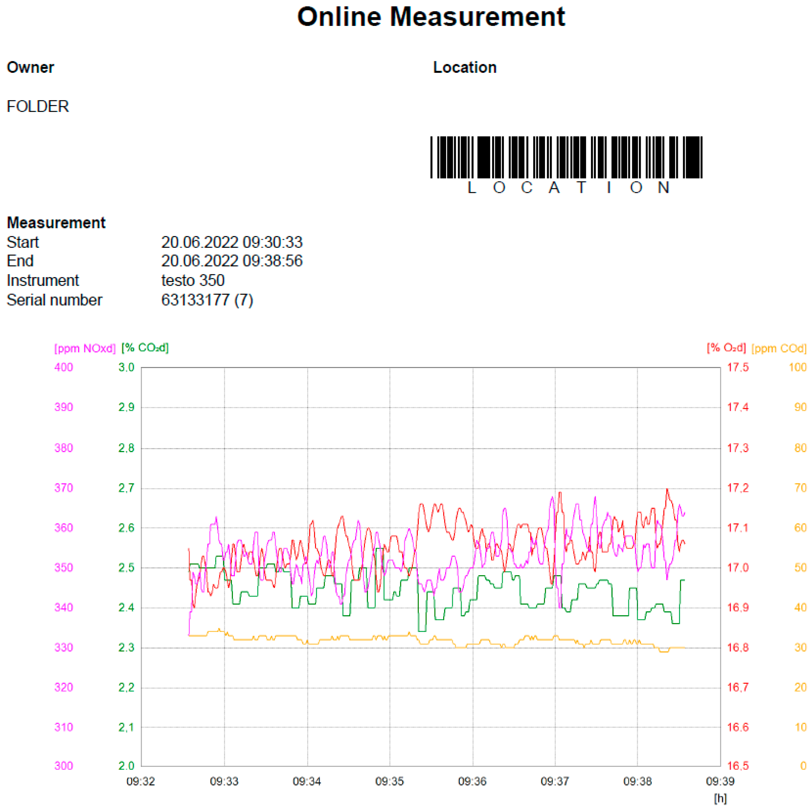
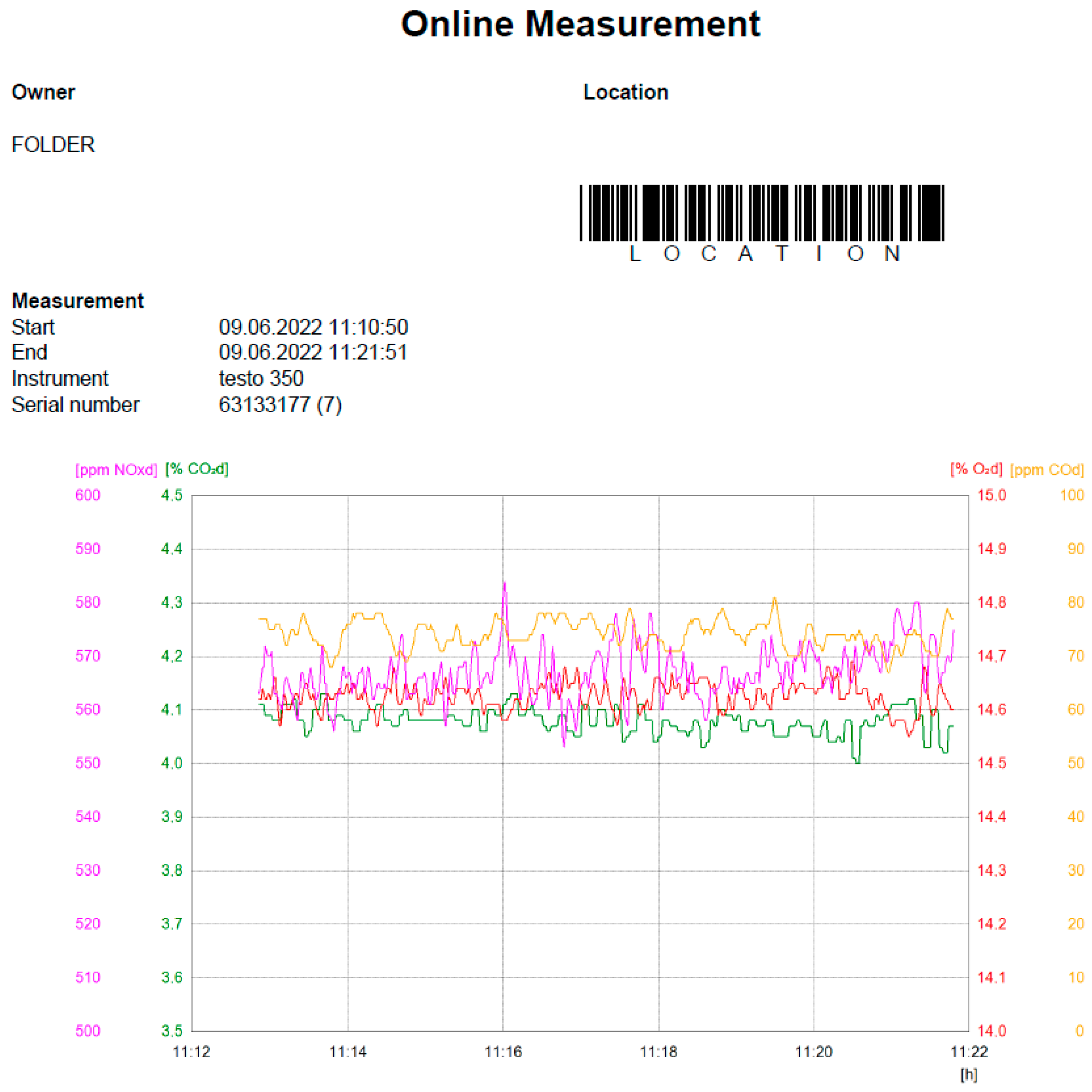
• The method of direct measurement of CO₂ emissions (Section 4.1) use a specialized device (Figure 4) with an emission transducer mounted on the engine exhaust system. The carbon balance method (Section 3.3 and Section 4.2) is used to convert direct measurements values into mass flow rates.
• The analytical method (Section 3.4 and Section 4.3), using experimentally determined formulas, involves employing equations derived from experimental data to calculate CO₂ emissions.
• The stoichiometric method (Section 3.5 and Section 4.4) for calculating the mass emissions of CO₂ from the exhaust gases can be applied if the carbon content of the used fuel and the fuel consumption per hour are known.

The gas emissions measurements were carried out on the exhaust gas systems of the engines during a voyage in the Mediterranean Sea from June to August 2022. The measurements were determined using the TESTO 350 MARITIME gas and emission analyzer shown in Figure 4. The device can be used to measure exhaust gas concentrations of NO, NO₂, SO₂, CO, CO₂-(IR), and O₂.

The measurement accuracy and range of the sensors are specified in Figure 5 and MARPOL annex VI and the NOx technical code [9]. The device consists of a control unit, a measuring probe, a memory unit, and a printer. The analyzer’s readings must not exceed ±2% of the measured value across the full measurement range (except zero) or ±0.3% of full scale, whichever is greater [9]. If a full CO₂ scale of 40% is taken, this means that the accuracy is 0.12% [9]. Because 0.12% is too low and irrelevant, it will be taken to 2% accuracy.

3.3. Carbon Balance Method for Calculating Emission Masses of CO₂

The carbon balance method [18,19] is used to determine the mass flow rates of exhaust gas emissions based on the measured data. This method could be used if there is information such as the exhaust gas concentrations of emissions, the engine combustion parameters, and the amount of fuel consumed by the engine for different loads. This method [20] consists of 12 sequential steps to be followed: determination of stoichiometric mixture, determination of the excess air coefficient, determination of the hydrogen-carbon ratio, determination of the absolute humidity of the supply air, determination of the saturation pressure of the water vapor in the supply air, determination of the absolute humidity of the scavenge air, determination of the saturation pressure of the water vapor in the scavenge air, determination of the dry/wet correction factors, determination of the exhaust gas mass flow rate, determination of the wet concentrations of the exhaust gas components, determination of the ratio between the densities of the exhaust gas components and the exhaust gas density, and determination of the mass flow rate of the exhaust gas components.

The amount of air requirement can be determined with the mathematical Equation (1) [8]:

$${ \mathrm{A}}_{\mathrm{S}}=\left({\displaystyle \frac{\mathrm{C}}{{\mathrm{M}}_{\mathrm{C}}}}+{\displaystyle \frac{\mathrm{H}}{4·{\mathrm{M}}_{\mathrm{H}}}}+{\displaystyle \frac{\mathrm{S}}{{\mathrm{M}}_{\mathrm{S}}}}\right)·{\displaystyle \frac{{\mathrm{M}}_{\mathrm{O}2}}{{\mathrm{M}}_{\mathrm{AO}2}}}\hspace{1em}\hspace{1em}\hspace{1em}\hspace{1em}\hspace{1em}\hspace{1em}\hspace{1em}\left[{\displaystyle \frac{\mathrm{kg} \mathrm{air}}{\mathrm{kg} \mathrm{fuel}}}\right]$$

(1)

Equation (1) [8] presents the following components:

C—carbon content of the fuel [%];

H—hydrogen content of the fuel [%];

S—sulfur content of the fuel [%];

M_C—molar mass of carbon [kg/mole];

M_H—molar mass of hydrogen [kg/mole];

M_S—molar mass of sulfur [kg/mole];

M_O2—molar mass of oxygen [kg/mole];

M_AO2—molar content of oxygen in the air [kg/mole];

The hydrogen—carbon ratio is determined using Equation (2) [8]:

$${\mathrm{R}}_{\mathrm{HC}}={\displaystyle \frac{\mathrm{H}·{\mathrm{M}}_{\mathrm{C}}}{\mathrm{C}·{\mathrm{M}}_{\mathrm{H}}}} \hspace{1em}\hspace{1em}\hspace{1em}\hspace{1em}\hspace{1em}\hspace{1em}\hspace{1em}\hspace{1em}\hspace{1em}\hspace{1em}\left[{\displaystyle \frac{\mathrm{mole} \mathrm{H}2}{\mathrm{mole} \mathrm{C}}}\right]$$

(2)

Equation (2) [8] presents the following components:

C—carbon content of the fuel [%];

H—hydrogen content of the fuel [%];

M_C—molar mass of carbon [kg/mole];

M_H—molar mass of hydrogen [kg/mole];

To determine the exhaust gas mass flow rate, Equation (3) is used [8]:

$${\mathrm{q}}_{\mathrm{me}\_\mathrm{w}}{ =\mathrm{C}}_{\mathrm{h}}·\left\{\left[{\displaystyle \frac{\frac{1.4 ·\left(\mathrm{C}·\mathrm{C}\right)}{\left(\frac{1.4· \mathrm{C}}{{\mathrm{f}}_{\mathrm{c}}}+\mathrm{H}· 0.08936—1\right)·\frac{1}{ 1.293}{+\mathrm{f}}_{\mathrm{fd}}}}{{\mathrm{f}}_{\mathrm{c}}·{ \mathrm{f}}_{\mathrm{c}}}}+\mathrm{C} · 0.08936-1\right]·\left(1+{\displaystyle \frac{{\mathrm{H}}_{\mathrm{a}}}{1000}}\right)+1\right\}$$

(3)

Equation (3) [8] presents the following components:

Ch—fuel consumption of the engine [kg fuel/h];

C—carbon content of the fuel [%];

H—hydrogen content of the fuel [%];

Ha—absolute humidity of the supply air [kg water/kg air];

N—nitrogen content of the fuel [%];

O—oxygen content of the fuel [%];

f_fd—fuel specific constant;

f_c—carbon factor;

The mass flow rate of the exhaust gas components is determined with Equation (4) [8]:

$${\mathrm{q}}_{\mathrm{gas}}={\mathrm{u}}_{\mathrm{gas}}·{\mathrm{c}}_{\mathrm{gas}\_\mathrm{w}}·{\mathrm{q}}_{\mathrm{me}\_\mathrm{w}}\hspace{1em}\hspace{1em}\hspace{1em}\hspace{1em}\hspace{1em}\hspace{1em}\left[{\displaystyle \frac{\mathrm{kg} \mathrm{gas}}{\mathrm{h}}}\right]$$

(4)

Equation (4) [8] presents the following components:

u_gas—the ratio between the density of the polluting component and the density of the exhaust gases;

c_{gas_w}—wet concentration of pollutant component in exhaust gases [ppm];

q_{me_w}—wet exhaust gas mass flow rate [Kg/h];

3.4. Analytical Method for Calculating Emission Masses of CO₂

The analytical method [21] is used to determine the mass flow rates of CO₂ emissions based on the oxidation mechanism of carbon in the fuel during combustion processes in the diesel engine.

The equation [8,22] for determining the CO₂ emission flow rate is as follows:

$${\mathrm{M}}_{\mathrm{CO}2}={\displaystyle \frac{{\mathrm{f}}_{\mathrm{CO}2 }·{ \mathrm{SFC}}_{\mathrm{engine}}·{ \mathrm{P}}_{\mathrm{engine}}}{1000}}\hspace{1em}\hspace{1em}\hspace{1em}\hspace{1em}\hspace{1em}\hspace{1em}\left[{\displaystyle \frac{{\mathrm{kg} \mathrm{CO}}_2}{\mathrm{h}}}\right]$$

(5)

Equation (5) [8,22] presents the following components:

f_CO2—the fuel conversion factor; for MDO is 3.2 kg CO₂/kg fuel;

SFC_engine—specific fuel consumption of the engine [g/kWh];

P_engine—engine power [kW];

3.5. Stoichiometric Method for Calculating Emission Masses of CO₂

This method, for calculating CO₂ emissions from burning one kilogram of fuel is based on the stoichiometric oxidation of the carbon from fuel composition. The chemical reaction is as follows:

$$\mathrm{C}+{\mathrm{O}}_2\to {\mathrm{CO}}_2+{\mathrm{Q}}_{\mathrm{C}}$$

(6)

Equation (6) presents the following components:

C—carbon mass in the fuel [kg C/Kg fuel];

O₂—the oxygen content of the air supply [kg O₂/kg air];

Qc—the resulting heat energy from the chemical reaction [Mj/kmole].

The stoichiometric Equation (7) for oxidation is usually expressed in kilomoles:

$$1 \mathrm{kmole} \mathrm{C}+1 \mathrm{kmole} \mathrm{O}2\to 1{ \mathrm{kmole} \mathrm{CO}}_2+{\mathrm{Q}}_{\mathrm{C}}$$

(7)

The reaction of carbon dioxide formation can be converted from kilomoles to kg by taking into account the molecular weight of carbon and oxygen as Equations (8) and (9):

$$12 \left[\mathrm{kgC}\right]+32 \left[{\mathrm{kgO}}_2\left] \to 44 \right[{\mathrm{kg} \mathrm{CO}}_2\right]$$

(8)

$$1\left[\mathrm{kgC}\right]+32/12 \left[{\mathrm{kgO}}_2\left] \to 44/\left(12\right) \right[{\mathrm{kg} \mathrm{CO}}_2\right]$$

(9)

For an amount of carbon burned “c” [kg C/kg fuel] from fuel, the combustion equation is as follows:

$$\mathrm{c} \left[\mathrm{kgC}\right]+{\displaystyle \frac{32\mathrm{C}}{12}}\left[{\mathrm{kgO}}_2\right]\to {\displaystyle \frac{44}{12}}\mathrm{c} \left[{\mathrm{kg} \mathrm{CO}}_2\right]$$

(10)

For a specified amount of fuel consumed over a defined time interval, the equation can be expressed as follows:

$${\mathrm{m}}_{\mathrm{CO}2}={\displaystyle \frac{44}{12}}·\mathrm{c}·{\mathrm{C}}_{\mathrm{h}}\hspace{1em}\hspace{1em}\hspace{1em}\hspace{1em}\hspace{1em}\hspace{1em}\hspace{1em}\hspace{1em}\hspace{1em}\hspace{1em}\left[{\displaystyle \frac{{\mathrm{kg} \mathrm{CO}}_2}{\mathrm{h}}}\right]$$

(11)

Equation (11) presents the following components:

Ch—hourly fuel consumption [kg fuel/h];

c—carbon contents in fuel.

4. Results

4.1. Measurement Performed Onboard the Ship

The measurements on board the ship were carried out by applying the measuring probe to the exhaust gas system of the engines. The measurements were performed with the ship underway, for three ship propulsion loads of 30%, 70%, and 90% from MCR (maximum continuous rating) and the operation of two diesel generators (auxiliary engines) at approximately 60% load. To extract the measurement results from the TESTO 350 marine device, the easyEmission v2.9 SP1—PC software was used.

Figure 6 includes the graph obtained from the TESTO measuring device for the main engine load of 30%. At 30% load, the engine operates at a partial power level, which can influence combustion efficiency and emissions. A reduced CO₂ value may indicate incomplete combustion, leading to increased emissions of CO (carbon monoxide), unburned hydrocarbons, and soot particles. If the measured CO₂ content is significantly lower than the theoretical value, it may indicate issues such as incorrect air-fuel mixture, carbon deposits, or low turbocharger efficiency. The measured value taken into account for theoretical analysis is the average value, as seen in Figure 7, over a certain time interval, when the main engine load has stabilized (constant load of 30%).

For 30% main engine load, the CO₂ level fluctuates within a relatively narrow range, approximately 2.38% to 2.55% over the course of the measurements, and the average value was considered 2.44%, as seen in Figure 7. To make the deviation diagrams as understandable as possible (Figure 7, Figure 8 and Figure 9), the measurement time interval was simplified and reduced to a measurement indicator. It is a reference used to distinguish more easily each individual measurement within a series of experimental data.

Figure 10 includes the graph obtained from the TESTO measuring device for the main engine load of 70%. At 70% load, the engine operates in a semi-optimized state, where combustion is more efficient than at lower loads (for example 30%). A high CO₂ value indicates complete and efficient combustion, with correct air intake, and a low CO₂ value may suggest incomplete combustion, leading to increased emissions of CO, unburned hydrocarbons, and soot particles. In addition, 70% load is considered ideal for diesel engines, as efficiency is high, and specific fuel consumption is optimal. The measured value taken into account for theoretical analysis is the average value over a certain time interval, when the main engine load has stabilized (constant load of 70%).

For 70% main engine load, the CO₂ level fluctuates within a relatively narrow range, approximately 3.31% to 4.38% over the course of the measurements, and the average value was considered 3.53%, as seen in Figure 8.

Figure 11 includes the graph obtained from the TESTO measuring device for the main engine load of 90%. At 90% load, the engine operates near maximum capacity, meaning a high combustion chamber temperature and greater efficiency. A high CO₂ value suggests that combustion is nearly complete, with an optimal air-fuel mixture, and a lower than theoretical CO₂ value may indicate combustion inefficiency, potential issues with fuel injection, or energy losses. At high loads, diesel engines reach peak performance, resulting in optimal CO₂ production and lower CO and HC emissions.

For 90% main engine load, the CO₂ level fluctuates within a relatively narrow range, approximately 3.31% to 4.38% over the course of the measurements, and the average value was considered 3.57%, as seen in Figure 8.

The obtained data and main engine operating parameters are listed in

Table 4. The measurements on board the ship for the main engine.

Parameter	Main Engine Load 30% 20 June 2022	Main Engine Load 70% 9 June 2022	Main Engine Load 90% 4 July 2022
Engine telegraph	Slow ahead	Half ahead	Full ahead
CPP angle [degree]	6	15	20
Engine speed [rpm]	350	355	365
Engine power [kW]	243	567	729
Fuel consumption [kg fuel/h]	52.245	121.905	156.735
CO2 [%]	$2.44 \pm 0.048$	$3.53 \pm 0.070$	$3.57 \pm 0.071$
O2 [%]	17.05	15.07	15.30
NOx [ppm]	353.2	516	478
CO [ppm]	31.96	47.74	45
SO2 [ppm]	25.34	29.22	27
Air temperature [°C]	25	25	25
Atmospheric pressure [hPa]	1018	1018	1018
Relative humidity [%]	50	50	50
Exhaust gas temperature [°C]	134.6	230.5	282.7
Fuel Sulphur quantity [%]	0.2	0.1	0.1

. The measured values taken into account are the average values over a certain time interval according to Figure 7, Figure 8 and Figure 9, when the main engine load has stabilized (constant load). The CO₂ values also include accuracy additions as seen in Table 4. Referring to Section 3.2 and Figure 5, 2% accuracy will be taken for the study. Table 4 also includes data such as engine power, engine speed, fuel consumption, exhaust gas temperature, atmosphere conditions, and emissions of CO₂, O₂, NOx, CO, and SO₂. As engine load increases (30% → 70% → 90%), the engine power scales up proportionally from 243 kW to 729 kW, and higher loads result in greater fuel consumption, climbing from 52.245 kg/h at 30% load to 156.735 kg/h at 90%. This means that the CO₂ concentrations rise with engine load, from 2.44% to 3.57%, indicating higher fuel combustion. Also, the measurements from the emissions analyzer are listed in Figure 6, Figure 10 and Figure 11.

Figure 12 includes the graph obtained from the TESTO measuring device for auxiliary engines load of 60%. For the auxiliary engines, three instant values of the amount of CO₂ were taken when they operated with a constant load of approximately 60% as seen in

Table 5. The measurements on board the ship for both diesel generators (cumulative emission).

Parameter	Load Approx. 60% 26 July 2022 16:52	Load Approx. 60% 26 July 2022 16:53	Load Approx. 60% 26 July 2022 16:54
Engine speed [rpm]	1500	1500	1500
Engine power [kW]	150	150	150
Fuel consumption [kg fuel/h]	31.05	31.05	31.05
CO2 [%]	$4.48 \pm 0.089$	$4.65 \pm 0.093$	$4.85 \pm 0.097$
O2 [%]	13.29	13.25	14.00
NOx [ppm]	731	736	709
CO [ppm]	155	165	163
SO2 [ppm]	43	39	41
Air temperature [°C]	25	25	25
Atmospheric pressure [hPa]	1018	1018	1018
Relative humidity [%]	50	50	50
Exhaust gas temperature [°C]	204.6	266.6	269.5
Fuel Sulphur quantity [%]	0.1	0.2	0.2

. The CO₂ values also include 2% accuracy additions.

The obtained data for both diesel generators (cumulative values) are listed in Table 5 and contain the same data type as the main engine. Engine speed remains constant at 1500 RPM and fuel consumption of 31.05 kg/h, indicating stable operation at this load. CO₂ levels gradually increase from 4.48% to 4.85%, suggesting a slight variation in combustion efficiency.

4.2. Results with Carbon Balance Method

To achieve this point, the data obtained from the experimental research presented in Table 4 and Table 5 are utilized, considering all three working loads of engines operation. It is the same tabular method applied to different engines shown in

Table 6. Table with the parameters needed for balance carbon calculation and the calculation results for ship main engine.

Parameter	Unit	Load 30%	Load 70%	Load 90%
Carbon content of fuel MDO	[%]	83.51	83.51	83.51
Hydrogen content of fuel MDO	[%]	13.30	13.30	13.30
Sulphur content of fuel MDO	[%]	0.077	0.077	0.077
Nitrogen content of fuel MDO	[%]	0.00	0.00	0.00
Oxygen content of fuel MDO	[%]	2.96	2.96	2.96
Molar mass of carbon	[kg/kmole]	12.011	12.011	12.011
Molar mass of hydrogen	[kg/kmole]	1.00797	1.00797	1.00797
Molar mass of sulfur	[kg/kmole]	32.060	32.060	32.060
Molar mass of oxygen	[kg/kmole]	31.999	31.999	31.999
Molar mass of air from oxygen	[kg/kmole]	23.15	23.15	23.15
Stoichiometric mixture requirement (STOIMIX)/100	[kg/kg]	0.1417	0.1417	0.1417
Molar volume of CO2	[dm3/mole]	22.262	22.262	22.262
Oxygen density	[kg/m3]	1.429	1.429	1.429
Molar volume of SO2	[dm3/mole]	21.891	21.891	21.891
Molar mass of nitrogen from air	[kg/kmole]	0.769	0.769	0.769
Nitrogen density	[kg/m3]	1.250	1.250	1.250
Excess air factor from CO2 (EAFCDO)	-	3.544	2.919	2.776
Hydrogen-carbon ratio (HTCRAT)	-	1.898	1.898	1.898
Suction air vapor pressure	[kPa]	3.17	3.17	3.17
Barometric pressure	[kPa]	101.3	101.3	101.3
Absolute humidity of suction air (AHA)	[g/kg]	9.88	9.88	9.88
Specific fuel factor for wet base (SFFW)	-	0.760106	0.760106	0.760106
Dry Air flow (Qmad)	[kg/h]	1749.65	5043.31	6166.82
H2 concentration	[%]	0.001045	0.001298	0.001488
Intake air temperature at air filter inlet (Ta)	[K]	298.15	298.15	298.15
Charge air temperature (T_sc)	[K]	298.75	298.75	298.75
Charge air temperature at each mode point corresponding to a seawater temperature of 25 °C (Specified by manufacturer) (T_SCRef)	[K]	296.75	296.75	296.75
Humidity correction factor for NOx for compression ignition engine (k_hd)	-	0.9844	0.9844	0.9844
Humidity correction factor for NOx for compression ignition engine with intercooler (k_hd)	-	0.9850	0.9850	0.9850
Charge air pressure (p_c)	[kPa]	10,130	10,130	10,130
Charge air vapor pressure (p_sc)	[kPa]	3.2822	3.2822	3.2822
Humidity of charging air	[g/kg]	0.2015956	0.2016	0.2016
Specific fuel factor (FFF)		0.0106571	0.0113605	0.0112089
CO2 concentration in ambient air	[%]	0.03	0.03	0.03
Carbon factor		1.3511	1.7869	1,9287
Specific fuel constant for dry exhaust (f_fd)		0.7601	0.7601	0.7601
Mass gas exhaust rate (q_mew)	[kg/h]	2766.5	7295.9	8680.9
Wet concentration—NOx	[ppm]	350.56	505.94	469.42
Wet concentration—O2	[%]	16.92	14.81	15.03
Wet concentration—CO	[ppm]	31.72	46.90	44.19
Wet concentration—CO2	[%]	2.42	3.47	3.51
Wet concentration—SO2	[ppm]	23.82	30.45	26.52
Density—NOx	[kg/m3]	2.053	2.053	2.053
Density—CO	[kg/m3]	1.25	1.25	1.25
Density—CO2	[kg/m3]	1.9636	1.9636	1.9636
Density—O2	[kg/m3]	1.4277	1.4277	1.4277
Density—HC	[kg/m3]	0.62	0.62	0.62
Density—SO2	[kg/m3]	2.855	2.855	2.855
Density—exhaust gas	[kg/m3]	1.2943	1.2943	1.2943
Ratio NOx density/exhaust gas density	-	0.000966	0.000966	0.000966
Ratio CO density/exhaust gas density	-	0.000479	0.000479	0.000479
Ratio HC density/exhaust gas density	-	0.001517	0.001517	0.001517
Ratio CO2 density/exhaust gas density	-	0.001103	0.001103	0.001103
Ratio O2 density/exhaust gas density	-	0.002206	0.002206	0.002206
Ratio SO2 density/exhaust gas density	-	0.000966	0.000966	0.000966
Mass flow—NOx	[kg/h]	2.3394	5.3987	6.3668
Mass flow—O2	[Kg/h]	79.7349	111.5392	143.8859
Mass flow—CO	[Kg/h]	0.130859	0.309364	0.370521
Mass flow—CO2	[Kg/h]	156.9387	359.3395	461.7545
Mass flow—SO2	[kg/h]	0.2244	0.4588	0.5078
Mass flow—wet air	[kg/h]	4.2193	6.7080	8.5247

and

Table 7. Table with the parameters needed for balance carbon calculation and the calculation results for ship auxiliary engines.

Parameter	Unit	Load 60%	Load 60%	Load 60%
Carbon content of fuel MDO	[%]	83.51	83.51	83.51
Hydrogen content of fuel MDO	[%]	13.30	13.30	13.30
Sulphur content of fuel MDO	[%]	0.077	0.077	0.077
Nitrogen content of fuel MDO	[%]	0.00	0.00	0.00
Oxygen content of fuel MDO	[%]	2.96	2.96	2.96
Molar mass of carbon	[kg/kmole]	12.011	12.011	12.011
Molar mass of hydrogen	[kg/kmole]	1.00797	1.00797	1.00797
Molar mass of sulfur	[kg/kmole]	32.060	32.060	32.060
Molar mass of oxygen	[kg/kmole]	31.999	31.999	31.999
Molar mass of air from oxygen	[kg/kmole]	23.15	23.15	23.15
Stoichiometric mixture requirement (STOIMIX)/100	[kg/kg]	0.1417	0.1417	0.1417
Molar volume of CO2	[dm3/mole]	22.262	22.262	22.262
Oxygen density	[kg/m3]	1.429	1.429	1.429
Molar volume of SO2	[dm3/mole]	21.891	21.891	21.891
Molar mass of nitrogen from air	[kg/kmole]	0.769	0.769	0.769
Nitrogen density	[kg/m3]	1.250	1.250	1.250
Excess air factor from CO2 (EAFCDO)	-	2.407	2.354	2.296
Hydrogen-carbon ratio (HTCRAT)	-	1.898	1.898	1.898
Suction air vapor pressure	[kPa]	3.17	3.17	3.17
Barometric pressure	[kPa]	101.3	101.3	101.3
Absolute humidity of suction air (AHA)	[g/kg]	9.88	9.88	9.88
Specific fuel factor for wet base (SFFW)	-	0.7601	0.7601	0.7601
Dry air flow (Qmad)	[kg/h]	1059.07	1035.74	1010.40
H2 concentration	[%]	0.004914	0.005231	0.005167
Intake air temperature at air filter inlet (Ta)	[K]	298.15	298.15	298.15
Charge air temperature (T_sc)	[K]	298.75	298.75	298.75
Charge air temperature at each mode point corresponding to a seawater temperature of 25 °C (Specified by manufacturer) (T_SCRef)	[K]	296.75	296.75	296.75
Humidity correction factor for NOx for compression ignition engine (k_hd)	-	0.9844	0.9844	0.9844
Humidity correction factor for NOx for compression ignition engine with intercooler (k_hd)	-	0.9850	0.9850	0.9850
Charge air pressure (p_c)	[kPa]	10130	10130	10130
Charge air vapor pressure (p_sc)	[kPa]	3.2822	3.2822	3.2822
Humidity of charging Air	[g/kg]	0.2015956	0.2016	0.2016
Specific fuel factor (FFF)		0.0110989	0.0110914	0.0110829
CO2 concentration in ambient air	[%]	0.03	0.03	0.03
Carbon factor		2.4296	2.5227	2.6314
Specific fuel constant for dry exhaust (f_fd)		0.7601	0.7601	0.7601
Mass gas exhaust rate (q_mew)	[kg/h]	1359.7	1308.6	1253.4
Wet concentration—NOx	[ppm]	711.80	715.54	688.02
Wet concentration—O2	[%]	12.94	11.91	13.59
Wet concentration—CO	[ppm]	150.93	160.41	158.18
Wet concentration—CO2	[%]	4.36	4.52	4.71
Wet concentration—SO2	[ppm]	41.87	37.92	39.79
Density—NOx	[kg/m3]	2.053	2.053	2.053
Density—CO	[kg/m3]	1.25	1.25	1.25
Density—CO2	[kg/m3]	1.9636	1.9636	1.9636
Density—O2	[kg/m3]	1.4277	1.4277	1.4277
Density—HC	[kg/m3]	0.620	0.620	0.620
Density—SO2	[kg/m3]	2.855	2.855	2.855
Density—exhaust gas	[kg/m3]	1.2943	1.2943	1.2943
Ratio NOx density/exhaust gas density	-	0.001586	0.001586	0.001586
Ratio CO density/exhaust gas density	-	0.000966	0.000966	0.000966
Ratio HC density/exhaust gas density	-	0.000479	0.000479	0.000479
Ratio CO2 density/exhaust gas density	-	0.001517	0.001517	0.001517
Ratio O2 density/exhaust gas density	-	0.001103	0.001103	0.001103
Ratio SO2 density/exhaust gas density	-	0.002206	0.002206	0.002206
Mass flow—NOx	[Kg/h]	1.5120	1.4629	1.3473
Mass flow—O2	[Kg/h]	19.4091	17.1906	18.7838
Mass flow—CO	[Kg/h]	0.198191	0.202727	0.191477
Mass flow—CO2	[Kg/h]	89.9857	89.7476	89.4980
Mass flow—SO2	[kg/h]	0.1256	0.1094	0.1100
Mass flow—wet air	[kg/h]	1.3286	1.2775	1.2224

. As can be seen in Table 6, the emissions were measured from concentrations of the total exhaust gas. To convert the concentrations into mass flow rates [23], the carbon balance method is used. The carbon balance calculation method [9] is used to assess the amount of carbon entering and leaving a system, ensuring mass conservation and tracking emissions or fuel efficiency. It is commonly applied in combustion processes, emissions analysis, and energy assessments. The carbon balance method can transform the concentration of CO₂ emissions, measured from engine exhaust gases, into mass flow rates. The fuel used is MDO with the characteristics according to Table 6. The table calculation starts from initial calculation data such as characteristics of the diesel components, mass participation of the fuel components, molar volume of the components, component densities, characteristics of the suction air, correction factors, and wet concentrations of components. Based on these initial data, according to the IMO—NOx Technical Code 2008 [9], the emission mass flows rates were calculated.

The same methodology will be applied for the auxiliary engines but for a single load of 60%. The carbon balance calculation values for auxiliary engines are listed in Table 7.

4.3. Results with Analytical Method

For diesel engines, the specific fuel consumption (SFC) varies depending on the engine load, following a parabolic pattern. Thus, at low loads, SFC tends to have higher values than the baseline; it then decreases to a minimum corresponding to a power level of 60–70% of the maximum power, after which it starts increasing again as the load rises. Therefore, the specific fuel consumption varies with load and can be determined using Equation (12), which was experimentally proven and is presented in the Fourth IMO Greenhouse Gas Study 2020 [10]. According to Equation (12) the specific fuel consumption is different depending on the engine load [24].

$${\mathrm{SFC}}_{\mathrm{load}}={\mathrm{SFC}}_{\mathrm{base}}\times \left(0.455\times {{ \mathrm{engine}}_{\mathrm{load}}}^2-0.71\times { \mathrm{engine}}_{\mathrm{load}}+1.280\right)$$

(12)

where SFCbase—baseline specific fuel consumption, dependent on the engine type, and

engine_load means engine load in % (respectively 30%, 70%, 90% for main engine and 60% for auxiliary engine).

The analytical method, as shown in Section 3.4, determines the main engine mass flow rates of CO₂ emissions depending on SFC_load, with values listed in

Table 8. Mass CO₂ emissions calculated with analytical method for main engine.

	Working Load of Engine
Mass	Load 1 30%	Load 2 70%	Load 3 90%
Kg CO2/h	185.2315	392.4171	506.3418

.

The same methodology will be applied for the auxiliary engines but for a single load of 60%. The analytical method calculation values for auxiliary engines are listed in

Table 9. Mass CO₂ emission calculated with analytical method for both diesel generators (cumulative values).

	Working Load of Engine
Mass	Load Approx. 60%
Kg CO2/h	101.13

.

4.4. Results with Stoichiometric Method

To calculate the amount of CO₂ emitted using the stoichiometric method, the methodology described in Section 3.5 was applied. The hourly fuel consumption for the main engine is shown in Table 4 and is calculated using the specific fuel consumption of 215 g/kWh according to the engine technical documentation. The carbon concentration in MDO fuel is 83.51%, as shown in Table 6. The calculated results are listed in

Table 10. Mass CO₂ emission calculated with stoichiometric method for main engine.

	Working Load of Engine
Mass	Load 1 30%	Load 2 70%	Load 3 90%
Kg CO2/h	160.6036	373.2771	479.9277

.

The same methodology was applied for the auxiliary engines. The hourly fuel consumption for both diesel generators is shown in Table 5 and was calculated using the specific fuel consumption of 207 g/kWh according to engine technical documentation. The carbon concentration in MDO fuel is 83.51%, as shown in Table 7. The calculated results are shown in

Table 11. Mass CO₂ emission calculated with stoichiometric method for both diesel generators (cumulative values).

	Working Load of Engine
Mass	Load Approx. 60%
Kg CO2/h	95.076

.

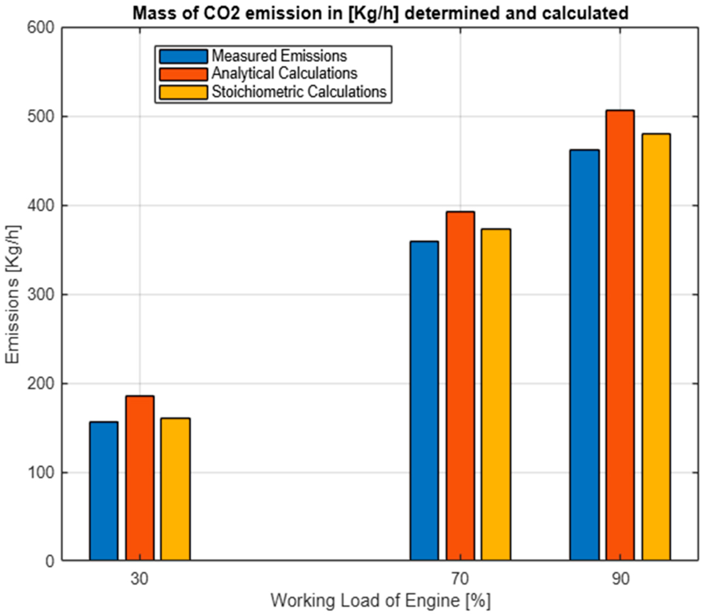
4.5. Comparative Results

The CO₂ masses determined experimentally (through measurements) and theoretically (analytical and stoichiometric) for the main engine are presented in

Table 12. Mass of CO₂ emission in [Kg/h] determined and calculated for main engine through the three methods.

Working Load of Engine	Measured Emission Mass Flow Rates [kg CO2/h]	Analytical Calculated Emission Mass Flow Rates [kg CO2/h]	Stoichiometric Calculated Emission Mass Flow Rates [kg CO2/h]
30%	156.9387	185.2315	160.6036
70%	359.3395	392.4171	373.2771
90%	461.7545	506.3418	479.9277

. Analyzing the results in Table 12 and the graph in Figure 13, the following aspects can be observed:

-

The highest value results are those obtained from the theoretical (analytical and stoichiometric) calculation;

-

The lowest value results are those obtained from the measurements carried out onboard the ship.

Experimentally measured values are the most relevant, as they reflect the actual efficiency of the engine under real operating conditions. They take into account factors such as combustion efficiency, internal losses, ambient conditions (temperature and humidity), and the technical condition of the engine. The stoichiometric method assumes complete and ideal combustion of the fuel, which provides a calculated estimate of the amount of CO₂ produced. Analytical calculations include all possible combustion scenarios, leading to maximum CO₂ emission values.

The CO₂ mass emissions determined experimentally (through measurements) and theoretically (analytical and stoichiometric) for diesel generators are presented in

Table 13. Mass of CO₂ emission in [Kg/h] determined and calculated for diesel generators (cumulative values).

Working Load of Engine	Measured Emission Mass Flow Rates [kg CO2/h]	Analytical Calculated Emission Mass Flow Rates [kg CO2/h]	Stoichiometric Calculated Emission Mass Flow Rates [kg CO2/h]
Approx. 60%	89.98	101.13	95.076
Approx. 60%	89.74	101.13	95.076
Approx. 60%	89.49	101.13	95.076

. Analyzing the results in Table 13 and the graph in Figure 14, the following aspects can be observed:

-

The highest value results are those obtained from the theoretically (analytical and stoichiometric) calculation;

-

The lowest value results are those obtained from the measurements carried out onboard the ship.

Comparing the three methods is valuable for improving engine design and compliance with emission limits imposed by international regulations. In practice, using all three methods in parallel can provide a complete perspective on emissions and help make informed decisions.

5. Discussion

The study is part of the global effort to combat climate change and protect the marine environment. This objective is particularly relevant for the maritime sector, given the significant role of maritime transport in global trade and its impact on the environment. Therefore, this paper aims to be a useful contribution to the general context of reducing GHG emissions, providing a theoretical and practical study model that can be applied to other similar ships.

The introductory analysis of this article was essential to understand the context in which efforts are undertaken to reduce CO₂ emissions. Without a clear understanding of global environmental issues, it is difficult to justify the need for specific measures in the maritime sector.

The aim of this article was to compare the results of carbon dioxide emission calculations derived from two theoretical methods with practical measurement data. It evaluated these calculation methods by assessing their accuracy against empirical emission measurements for diesel engines.

The measured values for the main engine at a maximum load of 90%, such as maximum 461.7545 kg CO₂/h, were lower than those calculated by theoretical methods (stoichiometric and analytical) with maximum 479.9277 kg CO₂/h and 506.3418 kg CO₂/h, as shown in Table 12, highlighting that idealized approaches did not fully reflect the complexity of the combustion process in reality. To better understand the differences in values, these have been converted into percentages.

Considering the observed discrepancies between the analytically calculated values and the real measurements, differences of 15.27%, 8.4%, and 8.8% for the three distinct main engine loads (30%, 70%, and 90%, respectively), it can be concluded that the measured emission values were consistently different than those calculated analytically for all assessed engine load levels. The observed discrepancy may indicate the influence of environmental factors such as efficiency losses or variations in operational parameters.

If the differences in values between the stoichiometric calculation and the real measurements (the differences of 2.2%, 3.73%, and 3.78% for main engine loads of 30%, 70%, and 90%, respectively) are taken into account, it can be concluded that the measured values were closer to stoichiometric, especially at low loads (30%), but show slightly larger differences at high engine loads (70%, 90%).

In addition, considering the differences in values between the stoichiometric calculation and analytical calculation (the differences of 13.29%, 4.87%, and 5.21% for main engine loads of 30%, 70%, and 90%, respectively), it can be concluded that the stoichiometric calculation values are lower than the analytical ones. The observed discrepancy may be attributed to the inherent simplifications within stoichiometric models.

For auxiliary engines, since they operate at approximately 60% load, the interpretation of the results, as shown in Table 13, is easier. The measured values are around 89.5–89.9 kg CO₂/h and indicate a good consistency between measurements. They reflect the real operating conditions of the diesel generator. The analytical values were higher (101.13 kg CO₂/h), which suggested that the analytical model integrated theoretical losses or assumed slightly different conditions than the real ones. The stoichiometric values (95.076 kg CO₂/h) were intermediate between the measured and analytical values, assuming ideal combustion but without adjustments for real variables.

If the results obtained in the article are compared with the results obtained in similar articles, it is noticed that the results are close. If compared with [12], it is observed that the results obtained through measurements, taking into account the maximum load studied of 90% of the main engine, 461.75 kg CO₂/h, 2.94 kg CO₂/Kg fuel (taking into account the fuel consumption of 156.735 kg fuel/h), show a difference of approximately 17% (comparing with 3.58 kg CO₂/Kg fuel). In addition, if compared with [13], taking into account the specific flow mass of 0.59 kg CO2/kWh, 430.11 kg CO₂/h is obtained compared to 461.75 kg CO₂/h. This is a difference of approximately 7%.

At the same time, the aim of the paper was to provide a practical and detailed analysis of CO₂ emissions onboard a specific ship, using real data and operating scenarios.

The paperwork can be completed through further research methods [26,27] for emissions reduction (for example, modification of fuel injection timing, selective catalytic reduction systems, treatment of the air required for combustion, water–fuel emulsion using, injection timing changing); these pollutant and simulation methods can also be introduced regarding the CO₂ emitted during the combustion of MDO in diesel engines.

6. Conclusions

The measured values for the main engine were lower than those calculated by theoretical methods (stoichiometric and analytical). This underlined the importance of direct measurements to obtain accurate data. These can be caused by engine conditions (wear, configuration), the characteristics of the fuel used, and operational parameters. The same can be observed for the CO₂ values related to intermediate loads of the main engine.

The discrepancy from 8.8% to 15.27% between the measured emission values and those calculated analytically for the main engine may indicate real factors such as efficiency losses, variations in operating conditions, or conservative assumptions used in the analytical models.

The observed discrepancy, ranging from 2.2% to 3.78%, between the measured emission values and the stoichiometrically calculated values for main engine, while not substantial, suggests potential variations in real-world emissions. These deviations may be attributed to factors such as non-ideal combustion conditions, variations in fuel composition, or incomplete chemical reactions.

The discrepancy from 4.87% to 13.29% between the stoichiometric calculation and analytical calculation for the main engine may be a consequence of the simplifications in the stoichiometric models, which assume perfect combustion without taking into account real inefficiencies or adjustments included in the analytical calculations.

In addition, the values of CO₂ deviations at different loads demonstrate that main diesel engines achieve optimal combustion efficiency at higher loads. At lower loads (30%), incomplete combustion leads to higher variation in CO₂ levels, while fuller combustion at 90% load ensures greater stability in CO₂ production.

The data analyzed for auxiliary engines suggest that the diesel generator operates efficiently at approximately 60% load, and the measured values provide a true image of real emissions. Differences from analytical calculations can be explained by factors such as more conservative theoretical assumptions or variability in operating conditions, the last being the most eloquent.

Experimental measurements allow for adjustment and optimization of engine operation based on objective data. This is essential for compliance with emissions regulations. In addition, theoretical calculations help identify potential problems and risks related to excessive emissions and take measures to reduce them.

References

1. Climate Change—NASA Science. Available online: https://science.nasa.gov/climate-change/ (accessed on 21 March 2025).
2. The Paris Agreement|UNFCCC. Available online: https://unfccc.int/process-and-meetings/the-paris-agreement (accessed on 21 March 2025).
3. Yoro, K.O.; Daramola, M.O. CO2 Emission Sources, Greenhouse Gases, and the Global Warming Effect. In Advances in Carbon Capture: Methods, Technologies and Applications; Woodhead Publishing: Pretoria, South Africa, 2020; pp. 4–6. [Google Scholar] [CrossRef]
4. Sustainable Maritime Fuels—‘Fit for 55′ package: The FuelEU Maritime proposal|Think Tank|European Parliament. Available online: https://www.europarl.europa.eu/thinktank/en/document/EPRS_BRI(2021)698808 (accessed on 21 March 2025).
5. Global Warming of 1.5 °C. Available online: https://www.ipcc.ch/sr15/ (accessed on 21 March 2025).
6. International Maritime Organization. Amendments to the Technical Code on Control of Emission of Nitrogen Oxides from Marine Diesel Engines (NOx Technical Code 2008). 2010. Available online: https://wwwcdn.imo.org/localresources/en/KnowledgeCentre/IndexofIMOResolutions/MEPCDocuments/MEPC.177(58).pdf (accessed on 2 April 2025).
7. International Maritime Organization. Guidelines on the Method of Calculation of the Attained Energy Efficiency Design Index (eedi) for New Ships. 2012. p. 2. Available online: https://wwwcdn.imo.org/localresources/en/KnowledgeCentre/IndexofIMOResolutions/MEPCDocuments/MEPC.212(63).pdf (accessed on 2 April 2025).
8. Coşofreţ, D.; Bunea, M.; Popa, C. The Computing Methods for CO2 Emissions in Maritime Transports. Int. Conf. Knowl.-Based Organ. 2016, 22, 622–627. [Google Scholar] [CrossRef]
9. MARPOOL. NOx Technical Code (2008). Technical Code on Control of Emission of Nitrogen Oxides from Marine Diesel Engines. 2008. Available online: https://media.liscr.com/marketing/liscr/media/liscr/online%20library/maritime/nox%20technical%20code%202008,%20as%20amended.pdf (accessed on 8 May 2025).
10. Fourth Greenhouse Gas Study 2020. Available online: https://www.imo.org/en/OurWork/Environment/Pages/Fourth-IMO-Greenhouse-Gas-Study-2020.aspx (accessed on 21 March 2025).
11. Xin, R.; Zhai, J.; Liao, C.; Wang, Z.; Zhang, J.; Bazari, Z.; Ji, Y. Simulation Study on the Performance and Emission Parameters of a Marine Diesel Engine. J. Mar. Sci. Eng. 2022, 10, 985. [Google Scholar] [CrossRef]
12. Lim, S.; Park, J.; Lee, J.; Lee, D.; Oh, J. Carbon Dioxide Emission Characteristics and Operation Condition Optimization for Slow-Speed and High-Speed Ship Engines. Appl. Sci. 2024, 14, 6134. [Google Scholar] [CrossRef]
13. Salehin, L.; Limon, M.M.I.; Mehedi, I. A Comparison of CO2 Emission between Diesel-Fueled and Dual-Fueled Marine Engines. Available online: https://www.researchgate.net/publication/384695125_A_Comparison_of_CO2_Emission_between_Diesel-Fueled_and_Dual-Fueled_Marine_Engines (accessed on 2 June 2025).
14. Chivu, R.M.; Martins, J.; Popescu, F.; Gonçalves, M.; Uzuneanu, K.; Frătița, M.; Brito, F.P. Assessment of Engine Performance and Emissions with Eucalyptus Oil and Diesel Blends. Energies 2024, 17, 3528. [Google Scholar] [CrossRef]
15. Skoko, I.; Stanivuk, T.; Franic, B.; Bozic, D. Comparative Analysis of CO2 Emissions, Fuel Consumption, and Fuel Costs of Diesel and Hybrid Dredger Ship Engines. J. Mar. Sci. Eng. 2024, 12, 999. [Google Scholar] [CrossRef]
16. Yuksel, O.; Pamik, M.; Bayraktar, M. The assessment of alternative fuel and engine power limitation utilisation in hybrid marine propulsion systems regarding energy efficiency metrics. J. Mar. Eng. Technol. 2025, 1–15. [Google Scholar] [CrossRef]
17. Forțele Navale Române. Available online: https://www.navy.ro/despre/bric/caract_nava.php (accessed on 13 June 2025).
18. Bhalothia, D.; Beniwal, A.; Bagaria, A.; Chen, T.-Y. Promoting CO2 Methanation Performance over NiO@TiO2 Nanoparticles via Oxygen Vacancies Enriched Fe-Oxide Modifiers Assisted Surface and Interface Engineering. Processes 2025, 13, 834. [Google Scholar] [CrossRef]
19. The Automotive Research Association of India. Chapter 8 Calculation of the Mass Emissions of Pollutants. DOC. No.: MoRTH/CMVR/TAP-115/116, no. Issue No. 4, 2010. Available online: https://www.araiindia.com/CMVR_TAP_Documents/Part-14/Part-14_Chapter08.pdf (accessed on 22 March 2025).
20. FPC International. Inc. Fuel Performance Catalyst—Technical Bulletins. Available online: https://www.fpc1.com/sci_cmb_fuel.php (accessed on 6 April 2025).
21. Sagin, S.; Haichenia, O.; Karianskyi, S.; Kuropyatnyk, O.; Razinkin, R.; Sagin, A.; Volkov, O. Improving Green Shipping by Using Alternative Fuels in Ship Diesel Engines. J. Mar. Sci. Eng. 2025, 13, 589. [Google Scholar] [CrossRef]
22. Third IMO GHG Study 2014 Executive Summary and Final Report. pp. 177–178, 2015. Available online: https://wwwcdn.imo.org/localresources/en/OurWork/Environment/Documents/Third%20Greenhouse%20Gas%20Study/GHG3%20Executive%20Summary%20and%20Report.pdf (accessed on 2 April 2025).
23. International Association of Classification Societies. Procedure for Calculation and Verification of the Energy Efficiency Design Index (EEDI). no. IACS Proc Req. 2013/Rev.3 2021. Available online: https://www.classnk.or.jp/hp/pdf/activities/statutory/eedi/16_pr38rev3.pdf (accessed on 22 March 2025).
24. Sadloe, A.; Rahnama, P.; Novella, R.; Somers, B. A Combined 1D/3D Method to Accurately Model Fuel Stratification in an Advanced Combustion Engine. Fire 2025, 8, 117. [Google Scholar] [CrossRef]
25. MATLAB Online, “MATLAB Home”. Available online: https://matlab.mathworks.com/?elqsid=vy8forrnvn46js7qemo6 (accessed on 1 April 2025).
26. Reitmayr, C.; Hofmann, P. Strategies to Increase Hydrogen Energy Share of a Dual-Fuel Hydrogen–Kerosene Engine for Sustainable General Aviation. Hydrogen 2025, 6, 17. [Google Scholar] [CrossRef]
27. Stipanov, M.; Dujmović, J.; Pelić, V.; Radonja, R. Simulation Approach as an Educational Tool for Comparing NOx Emission Reductions in Two-Stroke Marine Diesel Engines During Low-Load Operation: Water–Fuel Emulsion vs. Late Injection. Sustainability 2024, 16, 10833. [Google Scholar] [CrossRef]
Figure 1. Training ship.
Fire 08 00240 g001
Figure 2. The MAK 6 MU 451 main diesel engine used for ship propulsion.
Fire 08 00240 g002
Figure 3. The MAN D2866 auxiliary diesel engine.
Fire 08 00240 g003
Figure 4. Gas and emissions analyzer type TESTO 350 MARITIME.
Fire 08 00240 g004
Figure 5. TESTO 350 MARITIME accuracy.
Fire 08 00240 g005
Figure 6. Measurement no.1 for main engine with 30% load.
Fire 08 00240 g006
Figure 7. CO2 deviation from 2.44% (30% engine load).
Fire 08 00240 g007
Figure 8. CO2 deviation from 3.53% (70% engine load).
Fire 08 00240 g008
Figure 9. CO2 deviation from 3.57% (90% engine load).
Fire 08 00240 g009
Figure 10. Measurement no.2 for main engine with 70% load.
Fire 08 00240 g010
Figure 11. Measurement no.3 for main engine with 90% load.
Fire 08 00240 g011
Figure 12. Measurement no.1 for auxiliary engines.
Fire 08 00240 g012
Figure 13. Comparative analysis of measured and calculated CO2 emission masses for main engine made with MATLAB Online (basic) version [25] Software.
Fire 08 00240 g013
Figure 14. Comparative analysis of measured and calculated CO2 emission masses for diesel generators made with MATLAB Online [25] Software.
Fire 08 00240 g014