Kumaraswamy Generalized Power Lomax Distributionand Its Applications

Abstract

In this paper, a new five-parameter distribution is proposed using the functionalities of the Kumaraswamy generalized family of distributions and the features of the power Lomax distribution. It is named as Kumaraswamy generalized power Lomax distribution. In a first approach, we derive its main probability and reliability functions, with a visualization of its modeling behavior by considering different parameter combinations. As prime quality, the corresponding hazard rate function is very flexible; it possesses decreasing, increasing and inverted (upside-down) bathtub shapes. Also, decreasing-increasing-decreasing shapes are nicely observed. Some important characteristics of the Kumaraswamy generalized power Lomax distribution are derived, including moments, entropy measures and order statistics. The second approach is statistical. The maximum likelihood estimates of the parameters are described and a brief simulation study shows their effectiveness. Two real data sets are taken to show how the proposed distribution can be applied concretely; parameter estimates are obtained and fitting comparisons are performed with other well-established Lomax based distributions. The Kumaraswamy generalized power Lomax distribution turns out to be best by capturing fine details in the structure of the data considered.

1. Introduction

For several decades, researchers have been working to come up with several new distributions to meet certain practical requirements. The motivation is that, in concrete applications related to disciplines such as hydrology, econometrics and many others, the standard distributions have been observed to lack fit. For instance, for daily precipitation and daily vapor flow data, Kumaraswamy [1] showed that the beta distribution does not provide a suitable fit. Continuing this work, in References [2,3], it is also explored that distributions like Johnson, sinepower and extended sinepower distributions were satisfactory in fitting the above mentioned data type. However, in later years, an alternative distribution of finite range was suggested by Kumaraswamy [1] which is named later as Kw distribution. It reveals to fit such data appropriately. The cumulative distribution function (cdf) and probability density function (pdf) are given in (1) and (2), respectively:

$$F(x;a,b)=1-{(1-x^a)}^b,x\in (0,1),$$

(1)

and

$$f(x;a,b)=ab{x}^{a-1}{(1-x^a)}^{b-1},$$

(2)

where $a>0$ and $b>0$ are shape parameters, with the usual modifications for $x\notin (0,1)$. The main advantage of the Kw distribution is that it has the shape parameter that addresses data that has an extended tail nature. Also, the Kw distribution has been well received by many researchers for fitting skewed types of data sets from hydrology and other engineering disciplines. Other works on Kw distribution has been planned by several researchers, pointing out that it is a special case of the three-parameter beta distribution [4]. Also, the similarities along with basic properties have been extensively studied by Jones [5]. In the recent past, a generalized version of the Kw distribution has been proposed by Cordeiro and de Castro [6] with the cdf and pdf given in (3) and (4), respectively:

$$F_G(x;a,b)=1-{[1-G{\left(x\right)}^a]}^b,x\in \mathbb{R},$$

(3)

and

$$f_G(x;a,b)=abg\left(x\right)G{\left(x\right)}^{a-1}{[1-G{\left(x\right)}^a]}^{b-1}.$$

(4)

Here, $G\left(x\right)$ is the cdf of a chosen base distribution, with pdf given as $g\left(x\right)$. Clearly, if $a=b=1$, the forms in (3) and (4) reduce to the pdf and cdf from the base distribution. This generalized version of the Kw distribution is called the Kw-G family of distributions. Extensive work on the Kw-G family of distributions has been observed exponentially by proposing new distributions of various asymmetric natures. To cite a few, there are the Kumaraswamy-Weibull distribution [7], Kumaraswamy-Gumbel distribution [8], Kumaraswamy generalized gamma distribution [9] and Kumaraswamy-Burr XII (KBXII) distribution [10]. Applications of the Kw-G family can also be found in References [11,12,13], among others.

In general, the goal of providing new distributions is to create flexible mathematical models capable of handling non-normal data scenarios. This flexibility can be achieved in a simple way by adding additional parameters such as location, scale and shape. In similar lines of thought process, several distributions extending the famous Lomax distribution, such as the exponentiated-Lomax (EL) distribution [14], extended Lomax distribution [15], Kumaraswamy-generalized Lomax distribution [16], exponential-Lomax distribution [17], Weibull-Lomax (WL) distribution [18], Weibull Fréchet (WFr) distribution [19], power Lomax (PL) distribution [20], half-logistic Lomax distribution [21], inverse PL distribution [22], Topp-Leone Lomax (TLGL) distribution [23], type II Topp-Leone power Lomax (TIITLPL) distribution [24], Marshall-Olkin exponential Lomax distribution [25] and Marshall-Olkin length biased Lomax distribution [26] were proposed and developed.

In this present work, an attempt to propose a new distribution by compounding the PL distribution into the general Kw-G family of distributions is made. The proposed distribution is called the Kumaraswamy generalized PL distribution, KPL for short. The rationality of considering the PL distribution is that it equips the most famous extensions of the Lomax distribution [20] and it allows applications dealing with heavy tailed data. Because of its nature, we wish to exhibit mathematical flexibility by adding two additional shape parameters that are presented in the Kw-G family of distributions. To be more precise, a short retrospective on the PL distribution is necessary. First, let us mention that the cdf and pdf of the PL distribution have the forms in (5) and (6), respectively:

$$G(x;\alpha ,\beta ,\lambda )=1-{\left(\frac{\lambda }{\lambda +x^{\beta }}\right)}^{\alpha },x>0$$

(5)

and

$$g(x;\alpha ,\beta ,\lambda )=\frac{\alpha \beta x^{\beta -1}}{\lambda }{\left(\frac{\lambda }{\lambda +x^{\beta }}\right)}^{\alpha +1},$$

(6)

where $\alpha >0$ is a shape parameter, and $\beta >0$ and $\lambda >0$ are scale parameters. Rady et al. [20] mentioned that the hazard rate function (hrf) of the PL distribution does not have an increasing curve, which remains a serious limitation for some modeling purposes. This issue is addressed in this work by making the use of the shape parameter and it is performed in the proposed KPL distribution. In particular, the various forms of the pdf of the KPL distribution show that, with increasing values of the new parameters that will be denoted “a” and “b”, it is unimodal and can attain the symmetric nature curve. Also, the corresponding hrf possesses decreasing, increasing and inverted (upside-down) bathtub shapes. In addition, decreasing-increasing-decreasing shapes are observed, which is a clear plus for various statistical purposes. The KPL distribution and its statistical properties such as quantiles, moments, information measures, order statistics and maximum likelihood (ML) estimation are detailed out in subsequent sections of the article. Using two famous data sets, namely turbo charger data set and radiation therapy data set, we demonstrate that the proposed distribution is better suited compared to different types of Lomax distribution, including the PL distribution.

The rest of the article is structured by the following sections. Section 2 completes the presentation of the KPL distribution. Section 3 is devoted to its moments analysis. Section 4 is about information measures of the KPL distribution. Section 5 discusses the related order statistics. The estimation of the parameters of the KPL distribution is afforded in Section 6, including a simulation study. Section 7 focuses on the applications by considering two practical data sets. A summary is given in Section 8.

2. The Kumaraswamy Generalized Power Lomax Distribution

By considering (5) and (6) in (3) and (4), we obtain the following cdf and pdf, respectively,

$$F_{KPL}(x;\xi )=1-{\left\{1-{\left[1-{\left(\frac{\lambda }{\lambda +x^{\beta }}\right)}^{\alpha }\right]}^a\right\}}^b,x>0,$$

(7)

where $\xi =(\alpha ,\beta ,\lambda ,a,b)\in {(0,\infty )}^5$, and

$$f_{KPL}(x;\xi )=\frac{ab\alpha \beta }{\lambda }{x}^{\beta -1}{\left(\frac{\lambda }{\lambda +x^{\beta }}\right)}^{\alpha +1}{\left[1-{\left(\frac{\lambda }{\lambda +x^{\beta }}\right)}^{\alpha }\right]}^{a-1}{\left\{1-{\left[1-{\left(\frac{\lambda }{\lambda +x^{\beta }}\right)}^{\alpha }\right]}^a\right\}}^{b-1}.$$

(8)

The expressions (7) and (8) constitute the cdf and pdf of the KPL distribution, respectively. The KPL distribution contains several existing distribution, including the PL distribution for $a=b=1$ and the TIITLPL distribution for $a=2$. It can be also viewed as a re-parametrized version of the KBXII distribution. As already mentioned, the roles of a and b will be major in the interests of the KPL distribution, reaching new levels of flexibility compared to those of the PL distribution, among others.

As preliminary properties, note that $F_{KPL}(x;\xi )$ is a decreasing function with respect to a and $\lambda$, an increasing function with respect to b and $\alpha$, and a non-monotonic function with respect to $\beta$. This implies various first-order stochastic dominance properties. For instance, for ${\xi }_1=({\alpha }_1,\beta ,\lambda ,a,b_2)$ and ${\xi }_2=({\alpha }_2,\beta ,\lambda ,a,b_2)$ with ${\alpha }_1\le {\alpha }_2$ and $b_1\le b_2$, since $F_{KPL}(x;\xi )$ is an increasing function with respect to b and $\alpha$, we have $F_{KPL}(x;{\xi }_1)\le F_{KPL}(x;{\xi }_2)$. Similar inequalities can be presented by taking into account the other parameters. Also, it is worth mentioning that the KPL distribution is heavy-tailed; for all $t>0$, we can prove that ${\int }_0^{\infty }{e}^{tx}{f}_{KPL}(x;\xi )dx=\infty$.

Considering different values of the parameters, variant density forms of the KPL distribution are obtained, and are shown in Figure 1.

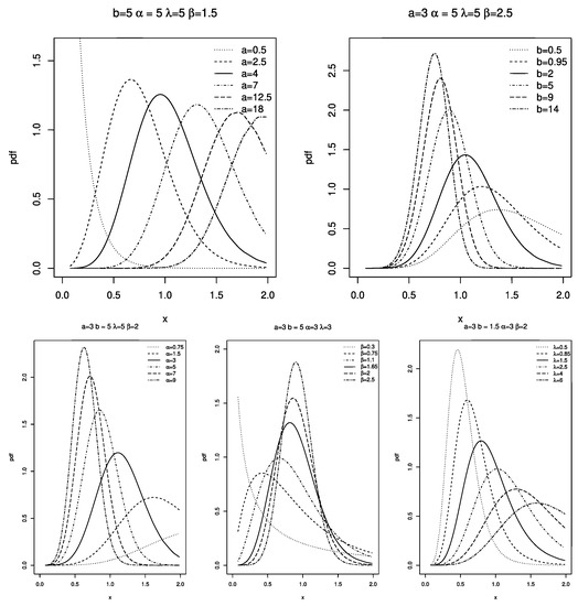
Figure 1. Curves of the pdf of the KPL distribution at different parameter values.

From Figure 1, we observe that the pdf of the KPL distribution can be decreasing or unimodal, with very flexible skewness, peakness and plateness. One can show that the decreasing case corresponds to $a\beta <1$. When the pdf is unimodal, we see that it is mainly ‘almost symmetric’ or ‘right-skewed’, which is ideal for the modelling of diverse lifetime phenomena.

Since the KPL distribution belongs to the family of lifetime distributions, its hrf is of interest to deals with some of the statistical properties of the proposed distribution. These properties will help out to exhibit the practical applications and characterizations of real data phenomenon. The hrf of the KPL distribution is given by

$$h_{KPL}(x;\xi )=\frac{f_{KPL}(x;\xi )}{1-F_{KPL}(x;\xi )},$$

that is, by substituting the Equations (7) and (8) in $h_{KPL}(x;\xi )$,

$$h_{KPL}(x;\xi )=\frac{ab\alpha \beta }{\lambda }{x}^{\beta -1}{\left(\frac{\lambda }{\lambda +x^{\beta }}\right)}^{\alpha +1}{\left[1-{\left(\frac{\lambda }{\lambda +x^{\beta }}\right)}^{\alpha }\right]}^{a-1}{\left\{1-{\left[1-{\left(\frac{\lambda }{\lambda +x^{\beta }}\right)}^{\alpha }\right]}^a\right\}}^{-1},x>0.$$

Considering various values of the parameters, the hrf of the KPL distribution contains different kinds of shapes as shown in Figure 2.

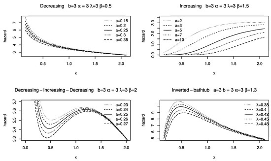
Figure 2. Shapes of the hrf of the KPL distribution at different parameter values.

From Figure 2, we highlight a crucial difference between the PL and KPL distributions. Indeed, an immediate limitation of the PL distribution is that its hrf cannot be increasing (see Reference [20]). This limitation is overcome in this work by using shape parameters and it is shown that the hrf of the proposed KPL distribution may be increasing. At the same time, we are able to present a decreasing-increasing-decreasing hrf. It is another point to emphasize that the proposed distribution has a better way of expressing different natures of data.

We end this part by presenting the quantile function (qf) of the KPL distribution which also defines it in the mathematical sense. This qf is rigorously defined as the inverse function of $F_{KPL}(x;\xi )$. By solving the following nonlinear equation: $F_{KPL}[Q_{KPL}(u;\xi );\xi ]=u$ with $u\in (0,1)$ and respect to $Q_{KPL}(u;\xi )$, we obtain

$$Q_{KPL}(u;\xi )={\lambda }^{1/\beta }{\left\{{\left[1-{\left(1-{(1-u)}^{1/b}\right)}^{1/a}\right]}^{-1/\alpha }-1\right\}}^{1/\beta },u\in (0,1).$$

We immediately derive the median of the KPL distribution as

$$M={\lambda }^{1/\beta }{\left\{{\left[1-{\left(1-{\left(0.5\right)}^{1/b}\right)}^{1/a}\right]}^{-1/\alpha }-1\right\}}^{1/\beta }.$$

Additional quantile analysis can be performed based on $Q_{KPL}(u;\xi )$. In this regard, one may refer to Reference [27].

3. Moments of the KPL Distribution

By definition, for any positive integer r, the $r^{th}$ order moment about the origin of a random variable X following the KPL distribution is given as

$${\mu }_r^{\prime }=E\left(X^r\right)={\int }_0^{\infty }{x}^r{f}_{KPL}(x;\xi )dx,$$

(9)

where E denotes the expectation. Clearly, in view of the mathematical complexity of $f_{KPL}(x;\xi )$, a simple expression of this integral is not possible. Let us first study its existence according to the values of the parameters of the KPL distribution. At the neighborhood of $x=0$, we have $f_{KPL}(x;\xi )\sim (ab{\alpha }^a\beta /{\lambda }^a)x^{\beta a-1}$ and, by the Riemann integrability criterion, since $r+\beta a>0$, the function $x^{r+\beta a-1}$ is integrable over $(0,ϵ)$ with $ϵ>0$. Now, at the neighborhood of $x=\infty$, we have $f_{KPL}(x;\xi )\sim a^{b}b\alpha \beta {\lambda }^{\alpha b}{x}^{-\beta \alpha b-1}$ and, by the Riemann integrability criterion, the function $x^{r-\beta \alpha b-1}$ is integrable over $(ϵ,\infty )$ with $ϵ>0$ if and only if $r<\beta \alpha b$. In summary, ${\mu }_r^{\prime }$ exists if and only if $r<\beta \alpha b$. In this case, one can approximate it via various numerical procedures.

For an analytical approach, one can derive series expansion for $f_{KPL}(x;\xi )$ and plug-in into (9). With this in mind, the next result presents a series expansion of a power transformation of the pdf of the KPL distribution.

Proposition 1.

For any $\rho >0$, we have

$$f_{KPL}{(x;\xi )}^{\rho }=\sum _{i=0}^{\infty }\sum _{j=0}^{\infty }{\upsilon }_{i,j}(\xi ,\rho )d_j(x;\alpha ,\beta ,\lambda ,\rho ),x>0,$$

where, by introducing generalized binomial coefficients,

$${\upsilon }_{i,j}(\xi ,\rho )={\left(\frac{ab\alpha \beta }{\lambda }\right)}^{\rho }\left(\genfrac{}{}{0pt}{}{\rho (b-1)}{i}\right)\left(\genfrac{}{}{0pt}{}{ai+\rho (a-1)}{j}\right){(-1)}^{i+j}$$

and

$$d_j(x;\alpha ,\beta ,\lambda ,\rho )=x^{\rho (\beta -1)}{\left(\frac{\lambda }{\lambda +x^{\beta }}\right)}^{\alpha j+\rho (\alpha +1)}.$$

Proof. 

We have

$$\begin{array}{cc}\hfill f_{KPL}{(x;\xi )}^{\rho }& ={\left(\frac{ab\alpha \beta }{\lambda }\right)}^{\rho }{x}^{\rho (\beta -1)}{\left(\frac{\lambda }{\lambda +x^{\beta }}\right)}^{\rho (\alpha +1)}{\left[1-{\left(\frac{\lambda }{\lambda +x^{\beta }}\right)}^{\alpha }\right]}^{\rho (a-1)}\times \hfill \\ \hfill & {\left\{1-{\left[1-{\left(\frac{\lambda }{\lambda +x^{\beta }}\right)}^{\alpha }\right]}^a\right\}}^{\rho (b-1)}.\hfill \end{array}$$

Now, the generalized binomial theorem states that ${(1-Z)}^b={\displaystyle \sum _{i=0}^{\infty }}\left(\genfrac{}{}{0pt}{}{b}{i}\right){(-1)}^i{Z}^i$ for any real numbers b and Z such that $\left|Z\right|<1$, condition that can be removed if b is a positive integer. Therefore, by the application of this theorem two times in a row, we obtain

$$\begin{array}{cc}\hfill f_{KPL}{(x;\xi )}^{\rho }& ={\left(\frac{ab\alpha \beta }{\lambda }\right)}^{\rho }{x}^{\rho (\beta -1)}{\left(\frac{\lambda }{\lambda +x^{\beta }}\right)}^{\rho (\alpha +1)}\sum _{i=0}^{\infty }\left(\genfrac{}{}{0pt}{}{\rho (b-1)}{i}\right){(-1)}^i{\left[1-{\left(\frac{\lambda }{\lambda +x^{\beta }}\right)}^{\alpha }\right]}^{ai+\rho (a-1)}\hfill \\ \hfill & ={\left(\frac{ab\alpha \beta }{\lambda }\right)}^{\rho }{x}^{\rho (\beta -1)}\sum _{i=0}^{\infty }\sum _{j=0}^{\infty }\left(\genfrac{}{}{0pt}{}{\rho (b-1)}{i}\right)\left(\genfrac{}{}{0pt}{}{ai+\rho (a-1)}{j}\right){(-1)}^{i+j}{\left(\frac{\lambda }{\lambda +x^{\beta }}\right)}^{\alpha j+\rho (\alpha +1)}\hfill \\ \hfill & =\sum _{i=0}^{\infty }\sum _{j=0}^{\infty }{\upsilon }_{i,j}(\xi ,\rho )d(x;\alpha ,\beta ,\lambda ,\rho ).\hfill \end{array}$$

The desired expansion is obtained. □

The particular case $\rho =1$ in Proposition 1 gives

$$f_{KPL}(x;\xi )=\sum _{i=0}^{\infty }\sum _{j=0}^{\infty }{\upsilon }_{i,j}(\xi ,1)d_j(x;\alpha ,\beta ,\lambda ,1).$$

Hence, under the condition that $r<\beta \alpha inf(b,1)$ permitting to interchange the integral and sum signs, the $r^{th}$ order moment about the origin of X is given as

$${\mathsf{\mu }}_r^{\prime }={\int }_0^{\infty }{x}^r\left[\sum _{i=0}^{\infty }\sum _{j=0}^{\infty }{\upsilon }_{i,j}(\xi ,1)d_j(x;\alpha ,\beta ,\lambda ,1)\right]dx=\sum _{i=0}^{\infty }\sum _{j=0}^{\infty }{\upsilon }_{i,j}(\xi ,1){\int }_0^{\infty }{x}^r{d}_j(x;\alpha ,\beta ,\lambda ,1)dx.$$

Let us now discuss a tractable expression for the integral term. We have

$$\begin{array}{c}\hfill {\int }_0^{\infty }{x}^r{d}_j(x;\alpha ,\beta ,\lambda ,1)dx={\int }_0^{\infty }{x}^{r+\beta -1}{\left(\frac{\lambda }{\lambda +x^{\beta }}\right)}^{\alpha (j+1)+1}dx.\end{array}$$

Let us now set $u=x^{\beta }/\lambda$, so $x={\left(u\lambda \right)}^{1/\beta }$ and $du=(\beta /\lambda )x^{\beta -1}dx$ with no change at the boundaries, implying that

$$\begin{array}{cc}\hfill & {\int }_0^{\infty }{x}^{r+\beta -1}{\left(\frac{\lambda }{\lambda +x^{\beta }}\right)}^{\alpha (j+1)+1}dx=\frac{\lambda }{\beta }{\int }_0^{\infty }\frac{{\left(u\lambda \right)}^{r/\beta }}{{(1+u)}^{\alpha (j+1)+1}}du\hfill \\ \hfill & =\frac{{\lambda }^{r/\beta +1}}{\beta }{\int }_0^{\infty }\frac{u^{(r/\beta +1)-1}}{{(1+u)}^{(r/\beta +1)+\left[\alpha \right(j+1)-r/\beta ]}}du=\frac{{\lambda }^{r/\beta +1}}{\beta }B\left(\frac{r}{\beta }+1,\alpha (j+1)-\frac{r}{\beta }\right),\hfill \end{array}$$

where $B(a,b)$ denotes the standard beta function defined by $B(a,b)={\int }_0^1{t}^{a-1}{(1-t)}^{b-1}dt$ with $a>0$ and $b>0$. We finally get

$${\mathsf{\mu }}_r^{\prime }=\sum _{i=0}^{\infty }\sum _{j=0}^{\infty }{\upsilon }_{i,j}(\xi ,1)\frac{{\lambda }^{r/\beta +1}}{\beta }B\left(\frac{r}{\beta }+1,\alpha (j+1)-\frac{r}{\beta }\right).$$

This formula is exact, without approximation. It can serve to determine the exact numerical values of ${\mathsf{\mu }}_r^{\prime }$ and all the associated measures. The most basic of them are the mean of X defined by ${\mathsf{\mu }}_1^{\prime }$ and the variance given by $Var={\mu }_2^{\prime }-{\left({\mu }_1^{\prime }\right)}^2$. A practical approximation of ${\mathsf{\mu }}_r^{\prime }$ is given by

$${\mathsf{\mu }}_r^{\prime }=\sum _{i=0}^{50}\sum _{j=0}^{50}{\upsilon }_{i,j}(\xi ,1)\frac{{\lambda }^{r/\beta +1}}{\beta }B\left(\frac{r}{\beta }+1,\alpha (j+1)-\frac{r}{\beta }\right),$$

the bound 50 being an integer chosen arbitrary large.

As an illustration, with the use of the R software, Table 1 provides the moments about the origin and variance of X with different parameter values of the KPL distribution.

Table 1. Moments about the origin and variance with different parameter values of the KPL distribution.

Parameters	a	${\mathsf{\mu }}_1^{\prime }$	${\mathsf{\mu }}_2^{\prime }$	${\mathsf{\mu }}_3^{\prime }$	${\mathsf{\mu }}_4^{\prime }$	$\mathbf{Var}$
$b=1$  $\alpha =2$   $\lambda =3$  $\beta =4$	1	1.096343	1.360350	1.898922	3.000000	0.1583815
	2	1.313328	1.870481	2.907724	5.000000	0.1456513
	3	1.434132	2.199940	3.641145	6.600000	0.1432048
	4	1.518195	2.448363	4.233660	7.971429	0.1434478
	5	1.582860	2.650083	4.738448	9.190476	0.1446359
$b=2$  $\alpha =4$   $\lambda =6$  $\beta =8$	1	0.9167115	0.8606779	0.8251498	0.8059774	0.020317974
	2	1.0286584	1.0695094	1.1233040	1.1912426	0.011371281
	3	1.0808945	1.1768814	1.2905014	1.4248888	0.008548480
	4	1.1137116	1.2475227	1.4053524	1.5920104	0.007169093
	5	1.1372247	1.2996238	1.4924269	1.7220834	0.006343810
$b=1.5$  $\alpha =1.5$   $\lambda =2$  $\beta =5$	1	0.9515346	0.9771163	1.075939	1.267621	0.07169832
	2	1.1398721	1.3609060	1.703722	2.242301	0.06159767
	3	1.2428513	1.6039652	2.154467	3.022583	0.05928593
	4	1.3141795	1.7859622	2.516701	3.691375	0.05889455
	5	1.3690008	1.9333437	2.824648	4.286271	0.05918053
$b=1.5$>   $\alpha =1.5$>   $\lambda =0.5$>   $\beta =2$	3	0.9246664	1.113072	1.936337	7.651063	0.2580643
	7	1.3393890	2.214626	5.046252	24.903052	0.4206629
	10	1.5452139	2.909026	7.447825	40.692316	0.5213404
	14	1.7598484	3.737898	10.690728	64.504585	0.6408318
	17	1.8937766	4.309344	13.141668	84.065516	0.7229542
$b=3.5$  $\alpha =0.8$   $\lambda =2.5$  $\beta =2$	3	2.381898	7.098448	27.62178	156.1513	1.425008
	7	4.209734	21.533759	141.10721	1329.5962	3.811897
	10	5.291480	33.862448	276.77366	3248.8381	5.862686
	14	6.547543	51.716382	520.95011	7533.2474	8.846066
	17	7.398181	65.967625	749.80026	12233.8552	11.234540
$b=2.7$  $\alpha =0.8$   $\lambda =0.5$  $\beta =2.2$	4	1.420161	2.542323	6.287137	28.97299	0.5254662
	11	2.573373	8.204595	35.761130	289.64094	1.5823481
	17	3.301047	13.473254	75.107768	778.33805	2.5763424
	22	3.822930	18.059557	116.502575	1397.61270	3.4447658
	36	5.056489	31.580735	269.364002	4275.42575	6.0126525

From Table 1, we see that the fourth moments about the origin and variance have notable numerical variations. This is particularly obvious for the last combination of parameters: $b=2.7$, $\alpha =0.8$, $\lambda =0.5$, $\beta =2.2$ with $a=4,11,17,22$ and 36. The high numerical variability of these moment measures also testifies to the flexibility of the KPL distribution.

The incomplete versions of the moments about the origin can have a similar mathematical treatment. They allow us to define various deviation measures and diverse types of residual life function, as those managed in References [10,20,24].

4. Information Measures

In this section, some information measures of the KPL distribution are discussed, namely the Rényi entropy and $\beta$-entropy measures. Both measuring the variation or uncertainty of the considered distribution.

4.1. Rényi Entropy

Rényi [28] provided an useful extension of the Shannon entropy. The Rényi entropy of the KPL distribution can be defined as

$$I_R^{\left(\rho \right)}=\frac{1}{1-\rho }log\left[{\int }_0^{\infty }{f}_{KPL}{(x;\xi )}^{\rho }dx\right],$$

with $\rho >0$ and $\rho \ne 1$. Let us now study the existence of this entropy measure which depends on the existence of its integral term. At the neighborhood of $x=0$, we have $f_{KPL}{(x;\xi )}^{\rho }\sim {(ab{\alpha }^a\beta /{\lambda }^a)}^{\rho }{x}^{\rho (\beta a-1)}$ and, by the Riemann integrability criterion, the function $x^{\rho (\beta a-1)}$ is integrable over $(0,ϵ)$ with $ϵ>0$ if and only if $\rho (\beta a-1)>-1$. Now, at the neighborhood of $x=\infty$, we have $f_{KPL}{(x;\xi )}^{\rho }\sim {\left[a^{b}b\alpha \beta {\lambda }^{\alpha b}\right]}^{\rho }{x}^{-\rho (\beta \alpha b+1)}$ and, by the Riemann integrability criterion, the function $x^{-\rho (\beta \alpha b+1)}$ is integrable over $(ϵ,\infty )$ with $ϵ>0$ if and only if $\rho (\beta \alpha b+1)>1$. Hence, $I_R^{\left(\rho \right)}$ exists if and only if $\rho (\beta a-1)>-1$ and $\rho (\beta \alpha b+1)>1$. If these conditions are satisfied, one can approximate $I_R^{\left(\rho \right)}$ through the approximation of its integral term via various numerical procedures.

In a more analytical manner, one can use Proposition 1. Under the conditions above plus $\rho (\beta -1)>-1$ and $\rho (\beta \alpha +1)>1$, a direct application of this result gives

$$\begin{array}{cc}\hfill {\int }_0^{\infty }{f}_{KPL}{(x;\xi )}^{\rho }dx& ={\int }_0^{\infty }\left[\sum _{i=0}^{\infty }\sum _{j=0}^{\infty }{\upsilon }_{i,j}(\xi ,\rho )d_j(x;\alpha ,\beta ,\lambda ,\rho )\right]dx\hfill \\ \hfill & =\sum _{i=0}^{\infty }\sum _{j=0}^{\infty }{\upsilon }_{i,j}(\xi ,\rho ){\int }_0^{\infty }{d}_j(x;\alpha ,\beta ,\lambda ,\rho )dx.\hfill \end{array}$$

A comprehensive expression of the integral term is developed below. By setting $u=x^{\beta }/\lambda$, so $x={\left(u\lambda \right)}^{1/\beta }$ and $du=(\beta /\lambda )x^{\beta -1}dx$ with no change at the boundaries, it comes

$$\begin{array}{cc}\hfill & {\int }_0^{\infty }{d}_j(x;\alpha ,\beta ,\lambda ,\rho )dx={\int }_0^{\infty }{x}^{\rho (\beta -1)}{\left(\frac{\lambda }{\lambda +x^{\beta }}\right)}^{\alpha j+\rho (\alpha +1)}dx\hfill \\ \hfill & =\frac{\lambda }{\beta }{\int }_0^{\infty }\frac{{\left(u\lambda \right)}^{(\rho -1)(1-1/\beta )}}{{(1+u)}^{\alpha j+\rho (\alpha +1)}}du\hfill \\ \hfill & =\frac{{\lambda }^{(\rho -1)(1-1/\beta )+1}}{\beta }{\int }_0^{\infty }\frac{u^{\left[\right(\rho -1\left)\right(1-1/\beta )+1]-1}}{{(1+u)}^{\alpha j+\rho (\alpha +1)-\left[\right(\rho -1\left)\right(1-1/\beta )+1]+\left[\right(\rho -1\left)\right(1-1/\beta )+1]}}du\hfill \\ \hfill & =\frac{{\lambda }^{(\rho -1)(1-1/\beta )+1}}{\beta }B\left[(\rho -1)\left(1-\frac{1}{\beta }\right)+1,\alpha j+\rho (\alpha +1)-(\rho -1)\left(1-\frac{1}{\beta }\right)-1\right].\hfill \end{array}$$

Therefore, we obtain an expression for $I_R^{\left(\rho \right)}$ as

$$\begin{array}{cc}\hfill I_R^{\left(\rho \right)}& =\frac{1}{1-\rho }log\{\sum _{i=0}^{\infty }\sum _{j=0}^{\infty }{\upsilon }_{i,j}(\xi ,\rho )\frac{{\lambda }^{(\rho -1)(1-1/\beta )+1}}{\beta }\times \hfill \\ \hfill & B\left[(\rho -1)\left(1-\frac{1}{\beta }\right)+1,\alpha j+\rho (\alpha +1)-(\rho -1)\left(1-\frac{1}{\beta }\right)-1\right]\}.\hfill \end{array}$$

This formula is exact, without approximation. The following simple approximation can be derived for practical purposes:

$$\begin{array}{cc}\hfill I_R^{\left(\rho \right)}& \approx \frac{1}{1-\rho }log\{\sum _{i=0}^{50}\sum _{j=0}^{50}{\upsilon }_{i,j}(\xi ,\rho )\frac{{\lambda }^{(\rho -1)(1-1/\beta )+1}}{\beta }\times \hfill \\ \hfill & B\left[(\rho -1)\left(1-\frac{1}{\beta }\right)+1,\alpha j+\rho (\alpha +1)-(\rho -1)\left(1-\frac{1}{\beta }\right)-1\right]\}.\hfill \end{array}$$

Here again, the bound 50 must be viewed as a large integer arbitrarily chosen.

4.2. Tsallis Entropy

The Tsallis entropy or q-entropy was discovered by Havrda and Charvat [29]. Later, it was developed by Tsallis [30] in the context of Physics. The Tsallis entropy of the KPL distribution can be defined as

$$I_H^{\left(q\right)}=\frac{1}{q-1}\left[1-{\int }_0^{\infty }{f}_{KPL}{(x;\xi )}^{q}dx\right],$$

where $q>0$ and $q\ne 1$. Then, based on the previous work on the Rényi entropy, $I_H^{\left(q\right)}$ exists if and only if $q(\beta a-1)>-1$ and $q(\beta \alpha b+1)>1$. In all cases, we can approximate it via numerical procedures. With the following additional assumptions: $q(\beta -1)>-1$ and $q(\beta \alpha +1)>1$, proceeding as for $I_R^{\left(\rho \right)}$, we can expand $I_H^{\left(q\right)}$ as

$$\begin{array}{cc}\hfill I_H^{\left(q\right)}& =\frac{1}{q-1}\{1-\sum _{i=0}^{\infty }\sum _{j=0}^{\infty }{\upsilon }_{i,j}(\xi ,q)\frac{{\lambda }^{(q-1)(1-1/\beta )+1}}{\beta }\times \hfill \\ \hfill & B\left[(q-1)\left(1-\frac{1}{\beta }\right)+1,\alpha j+q(\alpha +1)-(q-1)\left(1-\frac{1}{\beta }\right)-1]\right\}.\hfill \end{array}$$

Based on this formula, analytical approximation can be conducted.

5. Order Statistics

The modeling of certain random systems requires the concept of order statistic. Basically, for $r=1,\dots ,n$, the $r^{th}$ order statistic of a statistical sample is equal to its $r^{th}$ smallest value. In what follows, some immediate distributional properties of the order statistics of the KPL distribution are presented.

Let $X_{\left(1\right)},X_{\left(2\right)},\dots ,X_{\left(n\right)}$ be an ordered random sample distributed with the KPL distribution. Then, the pdf of $X_{\left(r\right)}$ is computed as

$$f_r(x;\xi )=\frac{1}{B(r,n-r+1)}{F}_{KPL}{(x;\xi )}^{r-1}{[1-F_{KPL}(x;\xi )]}^{n-r}{f}_{KPL}(x;\xi ),$$

that is, by substituting the Equations (7) and (8) in $f_r(x;\xi )$,

$$\begin{array}{cc}\hfill f_r(x;\xi )& =\frac{1}{B(r,n-r+1)}\frac{ab\alpha \beta }{\lambda }{x}^{\beta -1}{\left(\frac{\lambda }{\lambda +x^{\beta }}\right)}^{\alpha +1}{\left[1-{\left(\frac{\lambda }{\lambda +x^{\beta }}\right)}^{\alpha }\right]}^{a-1}\times \hfill \\ \hfill & {\left\{1-{\left[1-{\left(\frac{\lambda }{\lambda +x^{\beta }}\right)}^{\alpha }\right]}^a\right\}}^{b(n-r+1)-1}{\left[1-{\left\{1-{\left[1-{\left(\frac{\lambda }{\lambda +x^{\beta }}\right)}^{\alpha }\right]}^a\right\}}^b\right]}^{r-1},x>0.\hfill \end{array}$$

(10)

For $r=1$, we get the pdf of the first order statistics $X_{\left(1\right)}=min\left(X_1,X_2,\dots ,X_n\right)$ as follows

$$\begin{array}{cc}\hfill f_1(x;\xi )& =n\frac{ab\alpha \beta }{\lambda }{x}^{\beta -1}{\left(\frac{\lambda }{\lambda +x^{\beta }}\right)}^{\alpha +1}{\left[1-{\left(\frac{\lambda }{\lambda +x^{\beta }}\right)}^{\alpha }\right]}^{a-1}{\left\{1-{\left[1-{\left(\frac{\lambda }{\lambda +x^{\beta }}\right)}^{\alpha }\right]}^a\right\}}^{bn-1},x>0.\hfill \end{array}$$

One can remark that $f_1(x;\xi )=f_{KPL}(x;\alpha ,\beta ,\lambda ,a,bn)$, meaning that the distribution of $X_{\left(1\right)}$ is also a KPL distribution.

Similarly, for $r=n$, we get the pdf of the $n^{th}$ order statistics $X_{\left(n\right)}=max\left(X_1,X_2,\dots ,X_n\right)$ as follows

$$\begin{array}{cc}\hfill f_n(x;\xi )& =n\frac{ab\alpha \beta }{\lambda }{x}^{\beta -1}{\left(\frac{\lambda }{\lambda +x^{\beta }}\right)}^{\alpha +1}{\left[1-{\left(\frac{\lambda }{\lambda +x^{\beta }}\right)}^{\alpha }\right]}^{a-1}\times \hfill \\ \hfill & {\left\{1-{\left[1-{\left(\frac{\lambda }{\lambda +x^{\beta }}\right)}^{\alpha }\right]}^a\right\}}^{b-1}{\left[1-{\left\{1-{\left[1-{\left(\frac{\lambda }{\lambda +x^{\beta }}\right)}^{\alpha }\right]}^a\right\}}^b\right]}^{n-1},x>0.\hfill \end{array}$$

The next result exhibits the linear relation existing between the pdf of $X_{\left(r\right)}$ and some pdfs of the KPL distribution.

Proposition 2.

The pdf of $X_{\left(r\right)}$ can be expressed as a linear combination of pdfs of the KPL distribution, and, more precisely,

$$\begin{array}{c}\hfill f_r(x;\xi )=\frac{1}{B(r,n-r+1)}\sum _{k=0}^{r-1}\left(\genfrac{}{}{0pt}{}{r-1}{k}\right){(-1)}^k\frac{1}{n-r+k+1}{f}_{KPL}(x;\alpha ,\beta ,\lambda ,a,b(n-r+k+1)),x>0.\end{array}$$

Proof. 

It follows from (10) and the (standard) binomial theorem that

$$\begin{array}{cc}\hfill f_r(x;\xi )& =\frac{1}{B(r,n-r+1)}\frac{ab\alpha \beta }{\lambda }{x}^{\beta -1}{\left(\frac{\lambda }{\lambda +x^{\beta }}\right)}^{\alpha +1}{\left[1-{\left(\frac{\lambda }{\lambda +x^{\beta }}\right)}^{\alpha }\right]}^{a-1}\times \hfill \\ \hfill & {\left\{1-{\left[1-{\left(\frac{\lambda }{\lambda +x^{\beta }}\right)}^{\alpha }\right]}^a\right\}}^{b(n-r+1)-1}\sum _{k=0}^{r-1}\left(\genfrac{}{}{0pt}{}{r-1}{k}\right){(-1)}^k{\left\{1-{\left[1-{\left(\frac{\lambda }{\lambda +x^{\beta }}\right)}^{\alpha }\right]}^a\right\}}^{bk}\hfill \\ \hfill & =\frac{1}{B(r,n-r+1)}\sum _{k=0}^{r-1}\left(\genfrac{}{}{0pt}{}{r-1}{k}\right){(-1)}^k\frac{1}{n-r+k+1}\times \hfill \\ \hfill & \frac{ab(n-r+k+1)\alpha \beta }{\lambda }{x}^{\beta -1}{\left(\frac{\lambda }{\lambda +x^{\beta }}\right)}^{\alpha +1}{\left[1-{\left(\frac{\lambda }{\lambda +x^{\beta }}\right)}^{\alpha }\right]}^{a-1}\times \hfill \\ \hfill & {\left\{1-{\left[1-{\left(\frac{\lambda }{\lambda +x^{\beta }}\right)}^{\alpha }\right]}^a\right\}}^{b(n-r+k+1)-1}\hfill \\ \hfill & =\frac{1}{B(r,n-r+1)}\sum _{k=0}^{r-1}\left(\genfrac{}{}{0pt}{}{r-1}{k}\right){(-1)}^k\frac{1}{n-r+k+1}{f}_{KPL}(x;\alpha ,\beta ,\lambda ,a,b(n-r+k+1)).\hfill \end{array}$$

This ends the proof of Proposition 2. □

An immediate consequence of Proposition 2 is the determination of some properties for $X_{\left(r\right)}$ based on those of the KPL distribution. For example, the $s^{th}$ order moment of $X_{\left(r\right)}$ about the origin can be written as

$$\begin{array}{cc}\hfill {\mu }_{r,s}^{\prime }& =E\left(X_{\left(r\right)}^s\right)=\frac{1}{B(r,n-r+1)}\sum _{k=0}^{r-1}\left(\genfrac{}{}{0pt}{}{r-1}{k}\right){(-1)}^k\frac{1}{n-r+k+1}{\mu }_s^{\prime }\left(k\right),\hfill \end{array}$$

where ${\mathsf{\mu }}_s^{\prime }\left(k\right)$ denotes the $s^{th}$ order moment about the origin of a random variable with the KPL distribution with parameters $\alpha$, $\beta$, $\lambda$, a and $b(n-r+k+1)$.

6. Maximum Likelihood Estimates of the Parameters

The ML estimation method is used for estimating the unknown parameters of the distribution. Let $x=(x_1,x_2,\dots x_n)$ be a random sample drawn from the KPL distribution. Then the likelihood function and log-likelihood function corresponding to the Equation (8) are, respectively, as follows

$$L(x;\xi )={\left(\frac{ab\alpha \beta }{\lambda }\right)}^n\prod _{i=1}^n{x}_i^{\beta -1}{\left(\frac{\lambda }{\lambda +x_i^{\beta }}\right)}^{\alpha +1}{\left[1-{\left(\frac{\lambda }{\lambda +x_i^{\beta }}\right)}^{\alpha }\right]}^{a-1}{\left\{1-{\left[1-{\left(\frac{\lambda }{\lambda +x_i^{\beta }}\right)}^{\alpha }\right]}^a\right\}}^{b-1}$$

and

$$\begin{array}{cc}\hfill logL(x;\xi )& =nlog\left(\frac{ab\alpha \beta }{\lambda }\right)+(\beta -1)\sum _{i=1}^{n}log{x}_i+(\alpha +1)\sum _{i=1}^{n}log\left(\frac{\lambda }{\lambda +x_i^{\beta }}\right)+(a-1)\sum _{i=1}^{n}log{\vartheta }_i\hfill \\ \hfill & +(b-1)\sum _{i=1}^{n}log(1-{\vartheta }_i^a),\hfill \end{array}$$

where it is set ${\vartheta }_i=1-{\left[\lambda /(\lambda +x_i^{\beta })\right]}^{\alpha }$. The ML estimates (MLEs) of the parameters $a,b,\alpha ,\beta$ and $\lambda$, say $\widehat{a},\widehat{b},\widehat{\alpha },\widehat{\beta }$ and $\widehat{\lambda }$, are given by $\widehat{\xi }=(\widehat{a},\widehat{b},\widehat{\alpha },\widehat{\beta },\widehat{\lambda })$ making $L(x;\widehat{\xi })$ or $logL(x;\widehat{\xi })$ maximal. These MLEs can be obtained by solving the following nonlinear equations:

$$\frac{\partial }{\partial a}logL(x;\xi )=\frac{n}{a}+\sum _{i=1}^{n}log{\vartheta }_i+(1-b)\sum _{i=1}^n\frac{log{\vartheta }_i}{({\vartheta }_i^{-a}-1)}=0,$$

$$\frac{\partial }{\partial b}logL(x;\xi )=\frac{n}{b}+\sum _{i=1}^{n}log(1-{\vartheta }_i^a)=0,$$

$$\frac{\partial }{\partial \alpha }logL(x;\xi )=\frac{n}{\alpha }+\sum _{i=1}^{n}log\left(\frac{\lambda }{\lambda +x_i^{\beta }}\right)+\sum _{i=1}^n{\left(\frac{\lambda }{\lambda +x_i^{\beta }}\right)}^{\alpha }log\left(\frac{\lambda }{\lambda +x_i^{\beta }}\right)\left[\frac{a(b-1)}{{\vartheta }_i({\vartheta }_i^{-a}-1)}-\frac{(a-1)}{{\vartheta }_i}\right]=0,$$

$$\begin{array}{cc}\hfill \frac{\partial }{\partial \beta }logL(x;\xi )& =\frac{n}{\beta }+\sum _{i=1}^{n}log{x}_i-(\alpha +1)\sum _{i=1}^n\left(\frac{x_i^{\beta }}{\lambda +x_i^{\beta }}\right)\left[{\left(\frac{\lambda }{\lambda +x_i^{\beta }}\right)}^{\alpha -1}\frac{\lambda x_i^{\beta }log{x}_i}{{(\lambda +x_i^{\beta })}^2}\right]\times \hfill \\ \hfill & \left[\frac{\alpha (a-1)}{{\vartheta }_i}-\frac{a\alpha (b-1)}{{\vartheta }_i({\vartheta }_i^{-a}-1)}\right]log{x}_i=0\hfill \end{array}$$

and

$$\frac{\partial }{\partial \lambda }logL(x;\xi )=-\frac{n}{\lambda }+\left(\frac{\alpha +1}{\lambda }\right)\sum _{i=1}^n\left(\frac{x_i^{\beta }}{\lambda +x_i^{\beta }}\right)+\sum _{i=1}^n{x}_i^{\beta }{\left(\frac{\lambda }{\lambda +x_i^{\beta }}\right)}^{\alpha +1}\left[\frac{a\alpha (b-1)}{{\lambda }^2{\vartheta }_i({\vartheta }_i^{-a}-1)}-\frac{\alpha (a-1)}{{\lambda }^2{\vartheta }_i}\right]=0.$$

Based on data, the MLEs can be obtained numerically by the iterative procedure of Newton-Raphson method for a system of simultaneous nonlinear equations. As an example of use, Monte Carlo simulations are carried out to assess the finite sample behavior of the MLEs $\widehat{a}$, $\widehat{b}$, $\widehat{\alpha }$, $\widehat{\beta }$ and $\widehat{\lambda }$. For a given sample size, 1000 random samples drawn from the KPL distribution with given parameters are generated by using the qf technique. In this setting, the MLEs of the five model parameters along with the respective bias and mean square error (MSE) for the sample sizes $n=\{50,100,250\}$ are shown in Table 2.

Table 2. Bias in parenthesis and MSEs for different sample sizes in the context of the KPL distribution.

$(\mathit{a},\mathit{b},\mathit{\alpha },\mathit{\lambda },\mathit{\beta })$	$\widehat{\mathit{a}}$	$\widehat{\mathit{b}}$	$\widehat{\mathit{\alpha }}$	$\widehat{\mathit{\beta }}$	$\widehat{\mathit{\lambda }}$
$(10,4,5,0.5,20)$
$n=50$	(8.651935)	(6.67144)	(4.366995)	(−6.868542)	(1.093022)
	74.85599	44.50811	19.07065	47.17687	1.194697
$n=100$	(8.002526)	(4.365969)	(−2.73485)	(0.207459)	(−0.3513344)
	64.04406	19.08434	7.479976	0.08666441	0.1234489
$n=250$	(6.22343)	(−0.751908)	(−1.357911)	(2.745664)	(−0.3055339)
	38.73797	0.5679816	1.845981	7.551292	0.09335099
$(4,2,5,0.5,1.5)$
$n=50$	(−3.279042)	(−1.111076)	(−4.199035)	(3.525116)	(−0.4977061)
	10.75212	1.23449	17.6319	12.42645	0.2477113
$n=100$	(−3.003313)	(−0.9706962)	(−4.235572)	(0.7994587)	(−0.4568123)
	9.124203	1.134068	17.94019	0.641023	0.2086831
$n=250$	(−0.2668285)	(−1.074196)	(−2.093235)	(0.7068528)	(−0.4322879)
	0.07645446	1.187502	4.3866	0.4997061	0.1868756

As mentioned initially about the advantage of having additional shape parameters, the same is true between bias and MSE. From the results of Table 2, it is clearly evident that the estimates are quite stable and close to the true values of the parameters for these sample sizes. Additionally, as the sample size increases, the biases and MSEs of the MLEs decrease as expected.

7. Applications of the KPL Model

Two real data sets are used as applications of the proposed KPL distribution as heavy tailed distribution.

Data set 1: (Strength data [31]) The data represent 69 strength data for single carbon fibers (and impregnated 1000-carbon fiber tows). The measures in GPA by subtracting 1 are: 0.0312, 0.314, 0.479, 0.552, 0.700, 0.803, 0.861, 0.865, 0.944, 0.958, 0.966, 0.977, 1.006, 1.021, 1.027, 1.055, 1.063, 1.098, 1.140, 1.179, 1.224, 1.240, 1.253, 1.270, 1.272, 1.274, 1.301, 1.301, 1.359, 1.382, 1.382, 1.426, 1.434, 1.435, 1.478, 1.490, 1.511, 1.514, 1.535, 1.554, 1.566, 1.570, 1.586, 1.629, 1.633, 1.642, 1.648, 1.684, 1.697, 1.726, 1.770, 1.773, 1.800, 1.809, 1.818, 1.821, 1.848, 1.880, 1.954, 2.012, 2.067, 2.084, 2.090, 2.096, 2.128, 2.233, 2.433, 2.585, 2.585.

Data set 2: (Theft data [32]) The data represent the amounts of 120 theft claims made in a home insurance portfolio. The 120 theft claims data are: 3, 11, 27, 36, 47, 49, 54, 77, 78, 85, 104, 121, 130, 138, 139, 140, 143, 153, 193, 195, 205, 207, 216, 224, 233, 237, 254, 257, 259, 265, 273, 275, 278, 281, 396, 405, 412, 423, 436, 456, 473, 475, 503, 510, 534, 565, 656, 656, 716, 734, 743, 756, 784, 786, 819, 826, 841, 842, 853, 860, 877, 942, 942, 945, 998, 1029, 1066, 1101, 1128, 1167, 1194, 1209, 1223, 1283, 1288,1296, 1310, 1320, 1367, 1369, 1373, 1382, 1383, 1395, 1436, 1470, 1512, 1607, 1699, 1720, 1772, 1780, 1858, 1922, 2042, 2247, 2348, 2377, 2418, 2795, 2964, 3156, 3858, 3872, 4084, 4620, 4901, 5021, 5331, 5771, 6240, 6385, 7089, 7482, 8059, 8079, 8316, 11,453, 22,274, 32,043. After analyzing the histograms, data set 1 shows an offset deviation from the symmetrical pattern while data set 2 shows a decreasing histogram shape.

In order to show the best fit of the KPL distribution, some other distributions based on the Lomax distribution are considered and used for comparison. These competing distributions have already been mentioned in the introduction, and are the KBXII distribution [10], PL distribution [20], WL distribution [18], WFr distribution [19], TLGL distribution [23], EL distribution [14] and the basic Lomax distribution.

The ML estimation method is applied for all the distribution parameters. The MLEs are obtained by iterative procedures. The MLEs of the distribution parameters are given in Table 3.

Table 3. MLEs of the considered distribution parameters for the data sets.

Distribution Data Set 1	$\widehat{\mathit{a}}$	$\widehat{\mathit{b}}$	$\widehat{\mathit{\alpha }}$	$\widehat{\mathit{\lambda }}$	$\widehat{\mathit{\beta }}$
KPL	21.1082	6.5418	5.1957	0.4485	2.2026
KBXII	0.4342	0.2639	7.5759	1.9639	4.4371
PL		-	3.4574	13.5759	3.1625
WL	4.0405	2.711	0.7077	-	1.7575
WFr	6.4647	6.8652	0.7611	-	0.2297
TLGL	4.8177	-	12.3340	-	16.0790
EL	5.4551	-	21.9720	-	13.2469
Lomax	-	-	12.3594	-	17.9267
Distribution Data Set 2	$\widehat{\mathbf{a}}$	$\widehat{\mathbf{b}}$	$\widehat{\mathbf{\alpha }}$	$\widehat{\mathbf{\lambda }}$	$\widehat{\mathbf{\beta }}$
KPL	8.9953	7.4396	2.0506	5.5581	0.2604
WFr	0.0823	3.8303	5.0670	-	0.1522
WL	0.0056	0.1645	4.3790	-	1.2422
KBXII	8.3595	6.4601	0.0580	4.1935	1.5752
EL	6.1659	-	0.6294	-	17.4538
TLGL	9.5741	-	0.3008	-	7.2733
PL	-	-	0.9186	26.5070	0.5654
Lomax	-	-	0.2847	-	24.8517

Based on the notations of the KPL distribution, we now present the measures of adequacy that we use. Let $x_1,\dots ,x_n$ represent the data and $x_{\left(1\right)},\dots ,x_{\left(n\right)}$ be their ordered values. First, we consider the Cramér-von Mises (W*), Anderson Darling (A*) and Kolmogorov-Smirnov (K-S) statistics ($D_n$) defined by

$$\mathrm{W}*=\frac{1}{12n}+\sum _{i=1}^n{\left(F(x_{\left(i\right)};\widehat{\xi })-\frac{2i-1}{n}\right)}^2,$$

$$\mathrm{A}*=-n-\sum _{i=1}^n\frac{2i-1}{n}\left[log\left(F(x_{\left(i\right)};\widehat{\xi })\right)+log(1-F(x_i;\widehat{\xi }))\right]$$

and

$$D_n=\underset{i=1,\dots ,n}{max}\left(\frac{i}{n}-F(x_{\left(i\right)};\widehat{\xi }),F(x_{\left(i\right)};\widehat{\xi })-\frac{i-1}{n}\right),$$

respectively, where n is the sample size, $\xi$ denotes the parameters of the distribution ($\xi =(a,b,\alpha ,\beta ,\lambda )$ for the KPL distribution) and $\widehat{\xi }$ its vectorial MLE. The p-Value of the K-S test related to $D_n$ is also considered. The adequacy measures are widely used to know which distribution suits in a better manner. The distribution having the minimum value for the W* or A*, and maximum value for the p-Value, is chosen as the best one that is in adequacy to the data.

Also, we consider the Akaike information criterion (AIC), correct Akaike information criterion (CAIC), Bayesian information criterion (BIC) and Hannan-Quinn information criterion (HQIC), defined as

$$\begin{array}{cccc}\hfill \mathrm{AIC}& =-2logL(x;\widehat{\xi })+2k,\hfill & \hfill \mathrm{BIC}& =-2logL(x;\widehat{\xi })+klog\left(n\right),\hfill \\ \hfill \mathrm{CAIC}& =-2logL(x;\widehat{\xi })+\frac{2kn}{n-k-1},\hfill & \hfill \mathrm{HQIC}& =-2logL(x;\widehat{\xi })+2klog[log\left(n\right)],\hfill \end{array}$$

respectively, where k is the number of parameters ($k=5$ for the KPL distribution). As commonly accepted, the distribution having the minimum value for the AIC or CAIC or BIC or HQIC value is chosen as the best one that fits the data. For the considered data sets and distributions, the values of the measures above are computed and reported in Table 4.

Table 4. The goodness of fit tests and adequacy values for the data sets.

Distribution
Data Set 1	W*	A*	${\mathit{D}}_{\mathit{n}}$	p-Value	AIC	CAIC	BIC	HQIC
KPL	0.0232	0.2272	0.0604	0.9605	125.6272	126.5647	136.8697	130.0929
KBXII	0.0645	0.5108	0.0747	0.8287	129.838	130.7755	141.0804	134.3036
PL	0.1345	0.9450	0.0778	0.7909	131.9917	132.3553	138.7372	134.6711
WL	0.1860	1.2995	0.1030	0.4476	138.8186	139.4340	147.8126	142.3911
WFr	0.2186	1.4956	0.1205	0.2610	141.3542	141.9696	150.3482	144.9267
TLGL	0.4060	2.5291	0.1443	0.1085	152.7280	153.0916	159.4734	155.4073
EL	0.4265	2.6440	0.1440	0.1098	153.4122	153.7758	160.1577	156.0916
Lomax	0.3213	2.0540	0.3554	4.18 $\times {10}^{-08}$	204.3163	204.4954	208.8133	206.1026
Data Set 2	W*	A*	${\mathit{D}}_{\mathit{n}}$	p-Value	AIC	CAIC	BIC	HQIC
KPL	0.0936	0.4740	0.0726	0.5530	2035.768	2036.294	2049.705	2041.428
WFr	0.1523	0.8761	0.0957	0.2221	2039.442	2039.790	2050.592	2043.970
WL	0.1907	1.1122	0.1175	0.0730	2043.763	2044.111	2054.913	2048.292
KBXII	0.3134	1.7692	0.1558	0.0059	2060.251	2060.778	2074.189	2065.912
EL	0.5717	3.2453	0.1399	0.0182	2072.046	2072.252	2080.408	2075.442
TLGL	0.6155	3.5241	0.1372	0.0218	2077.853	2078.060	2086.215	2081.249
PL	0.1488	0.7585	0.2486	7.22 $\times {10}^{-7}$	2117.392	2117.599	2125.755	2120.788
Lomax	0.4167	2.3268	0.3110	1.65 $\times {10}^{-10}$	2157.868	2157.971	2163.443	2160.132

From the results of Table 4, it is evident that best fit is observed with the proposed KPL distribution and other distributions based on the Lomax distribution attained worst information criterion values. This is also witnessed through the fits of the pdfs that are depicted in Figure 3.

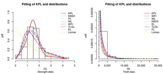
Figure 3. Fitted pdf curves of the distributions to the histograms for (a) data set 1 and (b) data set 2.

Among all the listed distributions, the KPL distribution has a better fit for the data considered. We confirm this visual result by plotting the Probability-Probability (PP) plots of the estimated distributions in Figure 4 and Figure 5 for data sets 1 and 2, respectively.

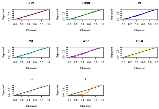
Figure 4. Fitted PP plots of the distributions for data set 1.

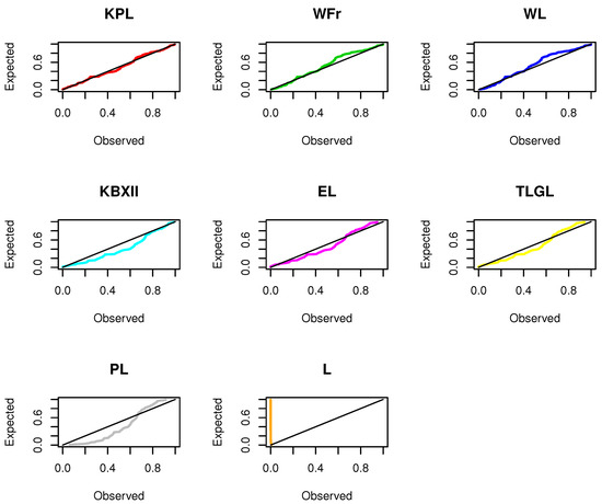
Figure 5. Fitted PP plots of the distributions for data set 2.

From Figure 4 and Figure 5, for the two data sets, it is clear that the best fit of the black diagonal line is assigned to the red line, corresponding to the one of the KPL distribution.

From these analyses, it can be seen that having additional shape parameters in the distribution is an advantage when talking about the extended tail version of the data. In addition, the dispersion and trend of the data can be characterized using the scale and location parameters of the basic distribution. Overall, a distribution that is compared to measurements of location, scale, and shape parameters always has a better advantage in handling non-normal data structures. Here, this advantage is captured by having two additional shape parameters which helped to see the characterization and fit in the best way.

8. Summary

The work carried out in this paper is to address some limitations of the PL distribution and also to illustrate the usefulness of the shape parameters in handling non-normal data. An attempt is made to introduce a new distribution, namely the KPL distribution, which is obtained by inducing the cdf of the PL distribution into the functional form of the Kw-G family of distributions. It contains five parameters consisting of one location, one scale and three shape parameters. In the work of Rady et al. [20], it is learned that the hrf of the PL distribution fails to attain the increasing pattern and decreasing-increasing-increasing pattern. This is not the case for the hrf of the KPL distribution. Important properties are studied, including moments, entropy measures and order statistics. With the help of two practical data sets, the fit of the KPL distribution is done. Information criterion measures are compared between the KPL distribution and some distributions also based on the Lomax distribution, including the PL distribution. It is shown that the KPL distribution has a better fit. Hence, the KPL distribution can work in a better manner for some kind of non-normal data.

References

- Kumaraswamy, P. A generalized probability density function for double-bounded random processes. J. Hydrol. 1980, 46, 79–88. [Google Scholar] [CrossRef]
- Kumaraswamy, P. Sinepower probability density function. J. Hydrol. 1976, 31, 181–184. [Google Scholar] [CrossRef]
- Kumaraswamy, P. Extended sinepower probability density function. J. Hydrol. 1978, 37, 81–89. [Google Scholar] [CrossRef]
- Nadarajah, S. On the distribution of Kumaraswamy. J. Hydrol. 2008, 348, 568–569. [Google Scholar] [CrossRef]
- Jones, M.C. Kumaraswamy’s distribution: A beta-type distribution with some tractability advantages. Stat. Methodol. 2009, 6, 70–81. [Google Scholar] [CrossRef]
- Cordeiro, G.M.; de Castro, M. A new family of generalized distributions. J. Stat. Comput. Simul. 2011, 81, 883–898. [Google Scholar] [CrossRef]
- Cordeiro, G.M.; Ortega, E.M.; Nadarajah, S. The Kumaraswamy Weibull distribution with application to failure data. J. Frankl. Inst. 2010, 347, 1399–1429. [Google Scholar] [CrossRef]
- Cordeiro, G.M.; Nadarajah, S.; Ortega, E.M. The Kumaraswamy Gumbel distribution. Stat. Methods Appl. 2012, 21, 139–168. [Google Scholar] [CrossRef]
- De Pascoa, M.A.; Ortega, E.M.; Cordeiro, G.M. The Kumaraswamy generalized gamma distribution with application in survival analysis. Stat. Methodol. 2011, 8, 411–433. [Google Scholar] [CrossRef]
- Paranaíba, P.F.; Ortega, E.M.; Cordeiro, G.M.; Pascoa, M.A.d. The Kumaraswamy Burr XII distribution: Theory and practice. J. Stat. Comput. Simul. 2013, 83, 2117–2143. [Google Scholar] [CrossRef]
- Malinova, A.; Golev, A.; Rahneva, O.; Kyurkchiev, V. Some notes on the Kumaraswamy-Weibull-Exponential cumulative sigmoid. Int. J. Pure Appl. Math. 2018, 120, 521–529. [Google Scholar]
- Malinova, A.; Kyurkchiev, V.; Iliev, A.; Kyurkchiev, N. A note on the transmuted Kumaraswamy quasi Lindley cumulative distribution function. Int. J. Sci. Res. Dev. 2018, 6, 561–564. [Google Scholar]
- Angelova, E.; Arnaudova, V.; Terzieva, T.; Malinova, A. A note on the new Kumaraswamy alpha power inverted exponential family of C.D.F. Neural Parallel Sci. Comput. 2020, 28, 59–67. [Google Scholar]
- Abdul-Moniem, I.B. Recurrence relations for moments of lower generalized order statistics from exponentiated Lomax distribution and its characterization. J. Math. Comput. Sci. 2012, 2, 999–1011. [Google Scholar]
- Lemonte, A.J.; Cordeiro, G.M. An extended Lomax distribution. Statistics 2013, 47, 800–816. [Google Scholar] [CrossRef]
- Shams, T.M. The Kumaraswamy-Generalized Lomax Distribution. Middle-East J. Sci. Res. 2013, 17, 641–646. [Google Scholar] [CrossRef]
- El-Bassiouny, A.H.; Abdo, N.F.; Shahen, H.S. Exponential Lomax Distribution. Int. J. Comput. Appl. 2015, 121, 24–29. [Google Scholar] [CrossRef]
- Tahir, M.H.; Cordeiro, G.M.; Mansoor, M.; Zubair, M. The Weibull-Lomax distribution: Properties and applications. Hacet. J. Math. Stat. 2015, 44, 461–480. [Google Scholar] [CrossRef]
- Afify, A.Z.; Yousof, H.M.; Cordeiro, G.M.; Ortega, E.M.; Nofal, Z.M. The Weibull Fréchet distribution and its applications. J. Appl. Stat. 2016, 43, 2608–2626. [Google Scholar] [CrossRef]
- Rady, E.H.A.; Hassanein, W.A.; Elhaddad, T.A. The power Lomax distribution with an application to bladder cancer data. SpringerPlus 2016, 5, 1–22. [Google Scholar] [CrossRef]
- Anwar, M.; Zahoor, J. The Half-Logistic Lomax Distribution for Lifetime Modeling. J. Probab. Stat. 2018, 3152807. [Google Scholar] [CrossRef]
- Hassan, A.S.; Abd-Allah, M. On the Inverse Power Lomax Distribution. Ann. Data Sci. 2019, 6, 259–278. [Google Scholar] [CrossRef]
- Oguntunde, P.E.; Khaleel, M.A.; Okagbue, H.I.; Odetunmibi, O.A. The Topp–Leone Lomax (TLLo) Distribution with Applications to Airbone Communication Transceiver Dataset. Wirel. Pers. Commun. 2019, 109, 349–360. [Google Scholar] [CrossRef]
- Al-Marzouki, S.; Jamal, F.; Chesneau, C.; Elgarhy, M. Type II Topp Leone Power Lomax Distribution with Applications. Mathematics 2020, 8, 4. [Google Scholar] [CrossRef]
- Nagarjuna, V.B.V.; Vardhan, V. Marshall-Olkin Exponential Lomax Distribution: Properties and its Application. Stoch. Model. Appl. 2020, 24, 161–177. [Google Scholar]
- Mathew, J.; Chesneau, C. Some New Contributions on the Marshall–Olkin Length Biased Lomax Distribution: Theory, Modelling and Data Analysis. Math. Comput. Appl. 2020, 25, 79. [Google Scholar] [CrossRef]
- Nair, N.U.; Sankaran, P.; Balakrishnan, N. Quantile-Based Reliability Analysis; Birkhäuser: Basel, Switzerland, 2013. [Google Scholar]
- Rényi, A. On Measures of Entropy and Information; Technical Report; Hungarian Academy of Sciences: Budapest, Hungary, 1961. [Google Scholar]
- Havrda, J.; Charvát, F. Quantification method of classification processes. Concept of structural a-entropy. Kybernetika 1967, 3, 30–35. [Google Scholar]
- Tsallis, C. Possible generalization of Boltzmann-Gibbs statistics. J. Stat. Phys. 1988, 52, 479–487. [Google Scholar] [CrossRef]
- Bader, M.; Priest, A. Statistical aspects of fibre and bundle strength in hybrid composites. In Progress in Science and Engineering Composites; Hayashi, T., Kawata, K., Umekawa, S., Eds.; ICCM-IV: Tokyo, Japan, 1982; pp. 1129–1136. [Google Scholar]
- Louzada-Neto, F.; Mazucheli, J.; Achcar, J.A. Uma Introdução à análise de Sobrevivência e Confiabilidade; Sociedad Chilena de Estadística: Valparaíso, Chili, 2001. [Google Scholar]
Publisher’s Note: MDPI stays neutral with regard to jurisdictional claims in published maps and institutional affiliations. |
© 2021 by the authors. Licensee MDPI, Basel, Switzerland. This article is an open access article distributed under the terms and conditions of the Creative Commons Attribution (CC BY) license (http://creativecommons.org/licenses/by/4.0/).