The Stacy-G Class: A New Family of Distributions with Regression Modeling and Applications to Survival Real Data

Abstract

We study the Stacy-G family, which extends the gamma-G class and provides four of the most well-known forms of the hazard rate function: increasing, decreasing, bathtub, and inverted bathtub. We provide some of its structural properties. We estimate the parameters by maximum likelihood, and perform a simulation study to verify the asymptotic properties of the estimators for the Burr-XII baseline. We construct the log-Stacy-Burr XII regression for censored data. The usefulness of the new models is shown through applications to uncensored and censored real data.

1. Introduction

In the last decades, there has been an increasing interest of articles in the context of new distributions. The ideas behind the generation of new families and, consequently, new distributions, are the most diverse possible, due to the transformation of a cumulative distribution function (cdf) to an integral of a probability density function (pdf) with an upper limit function, which follows some conditions [1]. However, even with the advancement in the area and the large number of publications, it is necessary to propose new distributions that fit more satisfactorily to real datasets. In this sense, our main objective is to study the properties of a new family that can present better fits to real data when compared to well consolidated classes.

The method of adding extra shape parameters to a cdf to generate more flexible distributions has been investigated by several authors over the last 20 years. The cdf of the generalized gamma (GG) pioneered by [2] is

$$F_s\left(w\right)=\frac{\gamma (a/b,{\left(cw\right)}^b)}{\Gamma (a/b)},w>0,$$

where $c>0$ is a scale parameter, $a>0$ and $b>0$ are the shape parameters, $\Gamma \left(a\right)={\int }_0^{\infty }{t}^{a-1}{\mathrm{e}}^{-t}dt$ is the complete gamma function, and $\gamma (a,z)={\int }_0^z{t}^{a-1}{\mathrm{e}}^{-t}dt$ is the lower incomplete gamma function. The generalized gamma model is also known as the Stacy distribution, say $\mathrm{S}(a,b,c)$. Table 1 lists some of its special cases.

Table 1. Stacy special distributions.

Distribution	a	b	c
Gamma	-	1	-
Weibull	b	a	-
Exponential	1	1	-
Rayleigh	2	2	-
Chi-square	$n/2$	1	$1/2$
Half-normal	1	2	$1/\left(k\sqrt{2}\right)$
Maxwell	3	2	$1/\left(k\sqrt{2}\right)$

de Pascoa et al. [3] defined the Kumaraswamy–Stacy, which extends the Kumaraswamy–Weibull [4], exponentiated-Stacy [5], exponentiated Weibull [6], among others. The beta-Stacy is another generalization introduced by [7], which includes 25 sub-models. Bourguignon et al. [8] proposed the truncated Stacy and showed that its hazard rate function (hrf) has five different shapes. Prataviera et al. [9] defined the odd log-logistic-Stacy (OLLS) distribution, which allows bathtub-shaped and unimodal hrf, and proposed a heteroscedastic log-OLLS regression to censored data. Ortega et al. [10] derived diagnostic measures to the Stacy regression, and [11] addressed this regression for long-term survivors.

Several families in the literature have emerged from well-known distributions, and provide more flexibility to the generated distributions, such as: odd log-logistic [12], Kumaraswamy [13], new extended-G [14], odd power Lindley [15], extended Weibull-G [16], Marshall–Olkin generalized G Poisson [17], generalized two-sided [18], generalized odd Weibull [19], odd log-logistic logarithmic [20], exponential Lindley odd log-logistic-G [21], odd Lomax [22], and odd Chen-G [23], among others. Two published distributions based in two previous families are: Kumaraswamy power Lomax [24] and odd log-logistic Birnbaum–Saunders–Poisson [25]. Some other classes based on the logarithmic transformation are the type I half-logistic [26], Gompertz [27], Weibull Marshall-Olkin [28], and xgamma [29].

Setting $c=1$ in the $\mathrm{S}(a,b,c)$ distribution, we define the cdf of the Stacy-G (SG) family (for a given parent G) by changing the argument w by the baseline cdf $G(x;\mathbf{\eta })$ with a q-vector of parameters $\mathbf{\eta }$

$$F_{\mathrm{SG}}\left(x\right)=\frac{\gamma (a/b,{\{-log[1-G(x;\mathbf{\eta })]\}}^b)}{\Gamma (a/b)}.$$

(1)

By differentiating (1), the SG density reduces to

$$\begin{array}{cc}\hfill f_{\mathrm{SG}}\left(x\right)=& \frac{b}{\Gamma (a/b)[1-G(x;\mathbf{\eta }\left)\right]}g(x;\mathbf{\eta }){\{-log[1-G(x;\mathbf{\eta })]\}}^{a-1}\hfill \\ & \times exp\{-{\{-log[1-G(x;\mathbf{\eta })]\}}^b\},\hfill \end{array}$$

(2)

where $g(x;\mathbf{\eta })=dG(x;\mathbf{\eta })/dx$.

Henceforth, the random variable $X\sim \mathrm{SG}(a,b,\mathbf{\eta })$ has density (2). For $b=1$, the SG family becomes the gamma-G class [30]. So, the Stacy family is a generalization of the gamma-G class with an extra shape parameter, thus providing greater flexibility to the density and failure rate functions. For $\delta =a/b$, Equation (2) is just Equation (10) of [30]. However, the last work does not investigate the structural properties of (2), which are obtained here from a linear representation. Further, a new reparametrization is provided in the context of regression. For $a=b=1$, it reduces to the parent G.

The hazard rate function (hrf) of X is

$$\begin{array}{c}\hfill {\tau }_{\mathrm{SG}}\left(x\right)=\frac{bg(x;\mathbf{\eta }){\{-log[1-G(x;\mathbf{\eta })]\}}^{a-1}{\mathrm{e}}^{-{\{-log[1-G(x;\mathbf{\eta })]\}}^b}}{\{\Gamma (a/b)-\gamma ((a/b),{\{-log[1-G(x;\mathbf{\eta })]\}}^b)\}[1-G(x;\mathbf{\eta })]}.\end{array}$$

We present four special models in Section 2. We derive a useful family density representation in Section 3, and obtain some properties in Section 4. In Section 5 and Section 6, we discuss the estimation of the parameters and Monte Carlo simulations, respectively. We define in Section 7 a new log-Stacy-Burr XII (LSBXII) regression. In Section 8, we prove the utility of the new models fitted to three real datasets. Finally, Section 9 concludes the paper.

2. Special Stacy-G Distributions

We present below four distributions generated by the Stacy-G family.

2.1. Stacy-Burr XII (SBXII)

Consider the parent Burr XII (BXII) cdf

$$G_{\mathrm{BXII}}\left(x\right)=1-{\left[1+{(x/s)}^c\right]}^{-d},$$

where all parameters are positive. The SBXII density (for $x>0$) follows from Equation (2) as

$$\begin{array}{cc}\hfill f_{\mathrm{SBXII}}\left(x\right)=& \frac{bc{d}^a}{s^c\Gamma (a/b)}{x}^{c-1}{\left[1+{(x/s)}^c\right]}^{-1}{\left\{log\left[1+{(x/s)}^c\right]\right\}}^{a-1}\hfill \\ & \times exp\left\{-{\{dlog[1+{(x/s)}^c]\}}^b\right\}.\hfill \end{array}$$

(3)

The SBXII reduces to the gamma-Burr XII (GBXII) [31] when $b=1$, gamma-Lomax [32] when $b=c=1$, and gamma-log-logistic [33] when $b=d=1$. Clearly, BXII ($a=b=1$), Lomax ($a=b=c=1$) and log-logistic ($a=b=d=1$) are well-known special distributions.

2.2. Stacy-Uniform (SU)

Inserting the cdf $G\left(x\right)$ and pdf $g\left(x\right)$ of the uniform, say $\mathrm{U}(c,d)$, in Equation (2), the SU density (for $-\infty <c<x<d<\infty$) comes as

$$\begin{array}{cc}\hfill f_{\mathrm{SU}}\left(x\right)=& \frac{b}{(d-x)\Gamma (a/b)}{\left\{-log\left(\frac{d-x}{d-c}\right)\right\}}^{a-1}{\mathrm{e}}^{-{\left\{-log\left(\frac{d-x}{d-c}\right)\right\}}^b}.\hfill \end{array}$$

It leads to the standard SU distribution when $c=0$ and $d=1$. The uniform $\mathrm{U}(c,d)$ distribution refers to $a=b=1$.

2.3. Stacy-Chen (SC)

The cdf and pdf of the Chen distribution (for $x>0$) are

$$G(x;\lambda ,\beta )=1-{\mathrm{e}}^{\lambda (1-{\mathrm{e}}^{x^{\beta }})}\mathrm{and}g(x;\lambda ,\beta )=\lambda \beta x^{\beta -1}{\mathrm{e}}^{x^{\beta }+\lambda (1-{\mathrm{e}}^{x^{\beta }})},$$

respectively, where $\lambda >0$ is a scale and $\beta >0$ is a shape parameter.

Inserting these expressions into Equation (2), the pdf of the SC distribution follows as

$$f_{sc}(x;a,b,\lambda ,\beta )=\frac{b{\lambda }^a\beta }{\Gamma (a/b)}{x}^{\beta -1}{({\mathrm{e}}^{x^{\beta }}-1)}^{a-1}exp\{x^{\beta }-{[-\lambda (1-{\mathrm{e}}^{x^{\beta }})]}^b\}.$$

For $b=1$, the SC distribution becomes the gamma-Chen [34] distribution.

2.4. Stacy–Weibull (SW)

The cdf of the Weibull (for $x>0$) is $G_w\left(x\right)=1-{\mathrm{e}}^{-{\left(\beta x\right)}^{\alpha }}$, where $\alpha >0$ and $\beta >0$. The SW density can be expressed as

$$f_{\mathrm{SW}}\left(x\right)=\frac{b\alpha {\beta }^{a\alpha }}{\Gamma (a/b)}{x}^{a\alpha -1}{\mathrm{e}}^{-{\left(\beta x\right)}^{\alpha b}}.$$

The gamma-Weibull follows when $b=1$, whereas $a=b=1$ refers to the Weibull. The exponential and Rayleigh models are obtained when $a=b=\alpha =1$ and $a=b=1$ and $\alpha =2$, respectively.

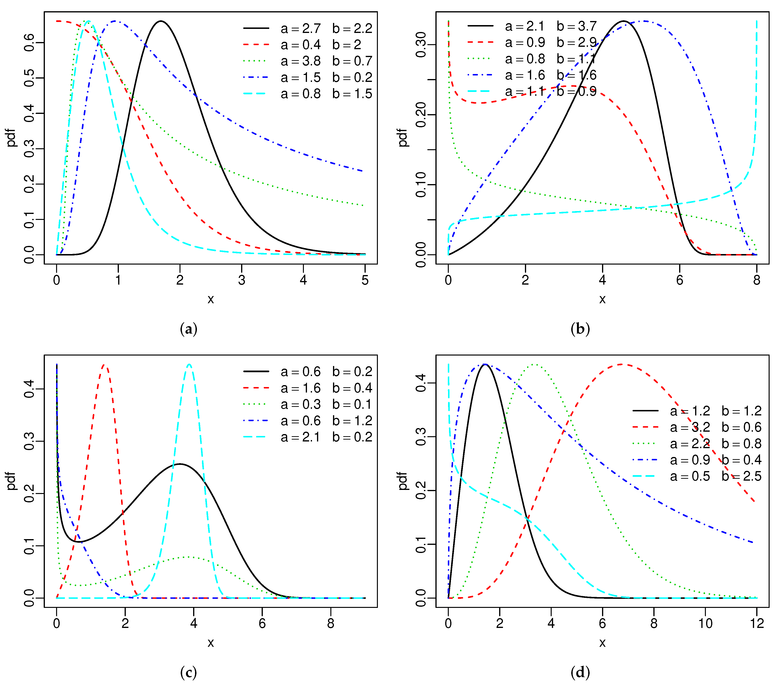
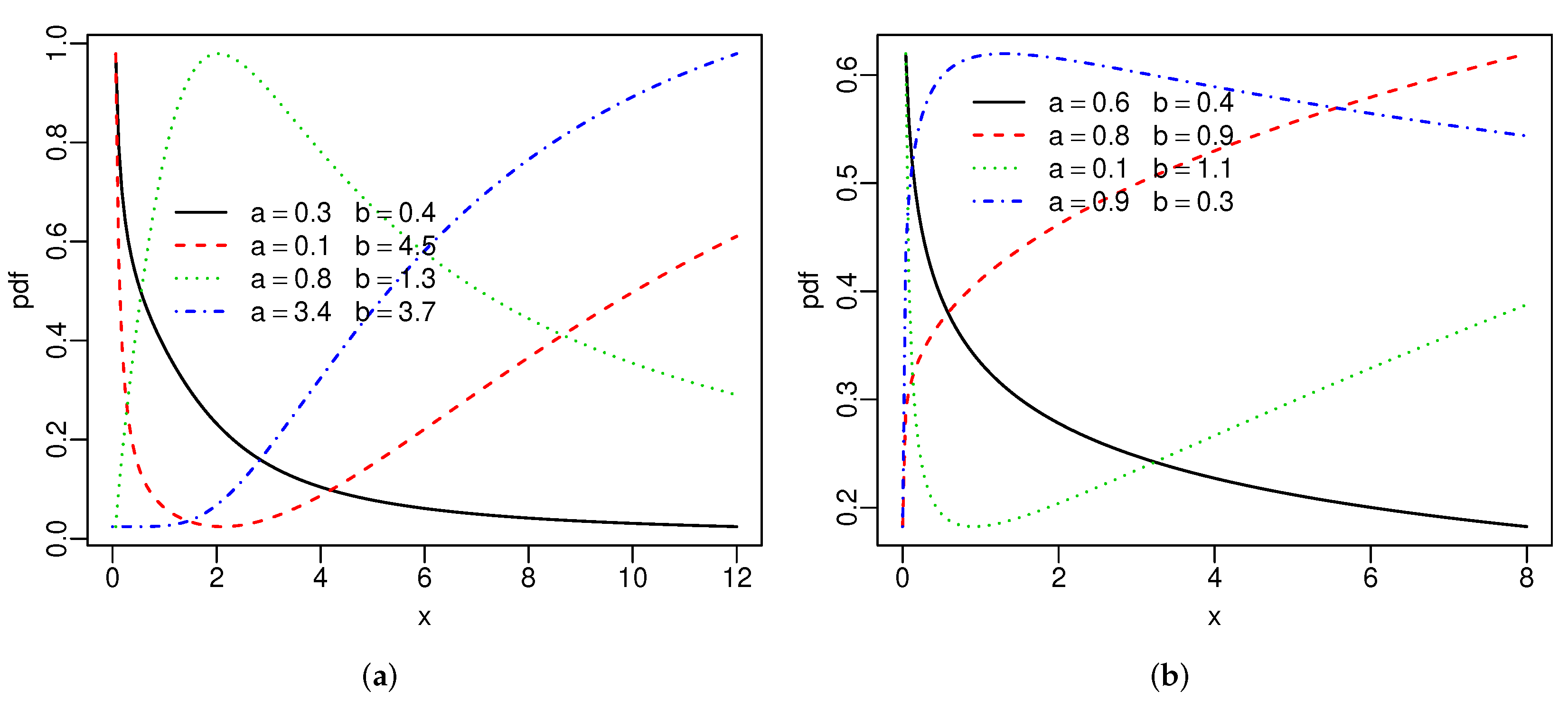
Figure 1 reports the above densities for fixed parameters. The two extra parameters provide more flexibility to these densities. Figure 2 gives the hrfs of the SBXII and SW models for specified parameters. For both models, the hrfs can be increasing, decreasing, bathtub, and inverse bathtub, thus showing that the extra shape parameters provide flexibility.

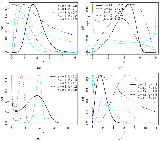
Figure 1. Special densities: (a) SBXII$(a,b,1.2,0.7,2.5)$, (b) SU$(a,b,0,8)$, (c) SC$(a,b,1.7,1.3)$ and (d) SW$(a,b,0.5,1.7)$.

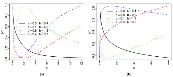
Figure 2. Special hrfs: (a) SBXII$(a,b,1.9,0.4,2.2)$ and (b) SW$(a,b,0.7,1.5)$ distributions.

The hrf of the GBXII [31] model can be decreasing, decreasing-increasing-decreasing, and inverse bathtub. The extra parameter b gives the possibility of two other forms for this hrf: increasing and bathtub. Hence, the SBXII distribution allows a greater variety of fits to different data sets than the GBXII model.

3. Linear Representation

Given a cdf $G(z;\mathbf{\eta })$ with a q-parameter vector $\mathbf{\eta }$, the random variable $Z_a\sim \exp -G(a,\mathbf{\eta })$ has the exponentiated-G (exp-G) density with power parameter $a>0$, say $h(z;a,\mathbf{\eta })=ag(z;\mathbf{\eta })G{(z;\mathbf{\eta })}^{a-1}$, where $g(z;\mathbf{\eta })=dG(z;\mathbf{\eta })/dz$. In the last 20 years, more than 35 exponentiated distributions have been published, and their structural properties are well-known.

The power series holds

$$exp\{-{\{-log[1-G(x;\mathbf{\eta })]\}}^b\}=\sum _{j=0}^{\infty }\frac{{(-1)}^j}{j!}{\{-log[1-G(x;\mathbf{\eta })]\}}^{jb}.$$

Plugging the last expression in Equation (2) gives

$$\begin{array}{cc}\hfill f_{\mathrm{SG}}(x;a,b,\mathbf{\eta })=& \frac{b}{\Gamma (a/b)[1-G(x;\mathbf{\eta }\left)\right]}g(x;\mathbf{\eta })\hfill \\ & \times \sum _{j=0}^{\infty }\frac{{(-1)}^j}{j!}{\{-log[1-G(x;\mathbf{\eta })]\}}^{jb+a-1}.\hfill \end{array}$$

(4)

For $\left|z\right|<1$ and any real $a\ne 0$, the two expansions hold

$${(1-z)}^a=\sum _{m=0}^{\infty }{(-1)}^m\left(\genfrac{}{}{0pt}{}{a}{m}\right)z^m$$

(5)

and

$${[-log(1-z)]}^a=\sum _{n=0}^{\infty }{R}_n\left(a\right)z^{n+a}.$$

(6)

Here, $R_0\left(a\right)=1$ and $R_n\left(a\right)=a{\delta }_{n-1}(n+a-1)$ (for $n\ge 1$), and the coefficients ${\delta }_{n-1}(·)$ are Stirling polynomials given by [35]

$$\begin{array}{cc}\hfill {\delta }_{n-1}\left(w\right)=& \frac{{(-1)}^{n-1}}{(n+1)!}\left[T_n^{n-1}-\frac{(w+2)}{(n+2)}{T}_n^{n-2}+\frac{(w+2)(w+3)}{(n+2)(n+3)}{T}_n^{n-3}\right.\hfill \\ & \left.-\cdots +{(-1)}^{n-1}\frac{(w+2)(w+3)\cdots (w+n)}{(n+2)(n+3)\cdots \left(2n\right)}{T}_n^0\right],\hfill \end{array}$$

where $T_0^0=1$, $T_{n+1}^0=1\times 3\times \dots \times (2n+1)$, $T_{n+1}^n=1$, and

$$T_{n+1}^m=(2n+1-m)T_n^m+(n-m+1)T_n^{m-1}.$$

Thus, we can write from Equations (5) and (6)

$${[1-G(x;\mathbf{\eta })]}^{-1}=\sum _{m=0}^{\infty }G{(x;\mathbf{\eta })}^m$$

and

$${\{-log[1-G(x;\mathbf{\eta })]\}}^{jb+a-1}=\sum _{n=0}^{\infty }{R}_n(jb+a-1)G{(x;\mathbf{\eta })}^{n+jb+a-1}.$$

Inserting these expansions in Equation (4) and after some algebra

$$\begin{array}{cc}\hfill f_{\mathrm{SG}}(x;a,b,\mathbf{\eta })=& \sum _{j,m,n=0}^{\infty }{w}_{j,m,n}h(x;m+n+jb+a,\mathbf{\eta }),\hfill \end{array}$$

(7)

where $h(x;(m+n+jb+a),\mathbf{\eta })$ is the $\exp -G(m+n+jb+a,\mathbf{\eta })$ density and

$$w_{j,m,n}=w_{j,m,n}(a,b)=\frac{{(-1)}^{j}b{R}_n(jb+a-1)}{(m+n+jb+a)\Gamma (a/b)j!}.$$

According to (7), the SG density function is a linear combination of exp-G densities. So, some of its mathematical properties can be easily obtained from those of the exp-G distribution. In practice, the infinity can be changed by a number such as 20.

4. Mathematical Properties

Let $W\sim \mathrm{S}(a,b,1)$ and $Q_G(u;\mathbf{\eta })=G^{-1}(u;\mathbf{\eta })$ be the quantile function (qf) of G. The transformed random variable $X=Q_G(W;\mathbf{\eta })$ has density function (2), and qf

$$Q_{\mathrm{SG}}(u;a,b,\mathbf{\eta })=Q_G(1-exp\{-Q^{-1}{(a/b,1-u)}^{1/b}\};\mathbf{\eta }),0<u<1,$$

(8)

where $t=Q^{-1}(a,u)$, and $Q(a,t)=1-\gamma (a,t)/\Gamma \left(a\right)=u$. So, variates from the SG family can be simulated from (8).

Further, let $Z_{j,m,n}\sim \exp -G(m+n+jb+a,\mathbf{\eta })$ (for $m,n,j\ge 0$). Some properties of X can be obtained from those of $Z_{j,m,n}$ for at least 35 parents G.

For example, the pth ordinary moment of X is obtained from (7) as

$$\begin{array}{cc}\hfill \mathbb{E}\left[X^p\right]=& \sum _{j,m,n=0}^{\infty }{w}_{j,m,n}\mathbb{E}\left[Z_{j,m,n}^p\right]\hfill \\ \hfill =& \sum _{j,m,n=0}^{\infty }(m+n+jb+a)w_{j,m,n}{\int }_0^1{Q}_g{(u;\mathbf{\eta })}^p{u}^{m+n+jb+a-1}du.\hfill \end{array}$$

The moments of some generated models can be much simpler and practically hassle-free. For example, for the SW distribution, the pth moment is

$$\begin{array}{c}\hfill \mathbb{E}\left[X^p\right]=\frac{{\beta }^{\alpha (a-1)-p}\Gamma \left(\frac{p+\alpha }{b\alpha }\right)}{\Gamma \left(\frac{a}{b}\right)}.\end{array}$$

Further, the generating function (gf) of X comes from (7) as

$$\begin{array}{cc}\hfill M_X\left(t\right)=& \sum _{j,m,n=0}^{\infty }{w}_{j,m,n}{M}_{j,m,n}\left(t\right)\hfill \\ \hfill =& \sum _{j,m,n=0}^{\infty }(m+n+jb+a)w_{j,m,n}{\int }_0^1{\mathrm{e}}^{t{Q}_g(u;\mathbf{\eta })}{u}^{m+n+jb+a-1}du,\hfill \end{array}$$

where $M_{j,m,n}\left(t\right)$ is the gf of $Z_{j,m,n}$.

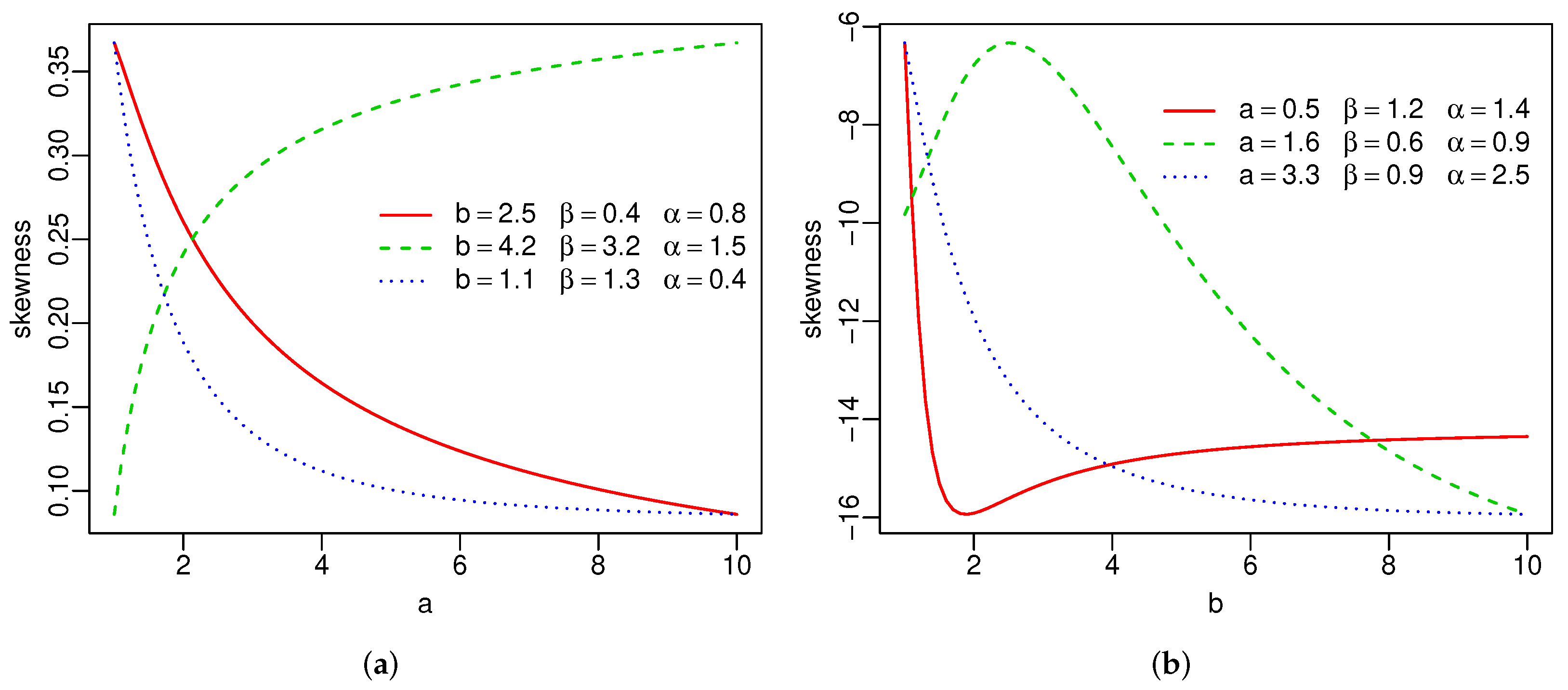
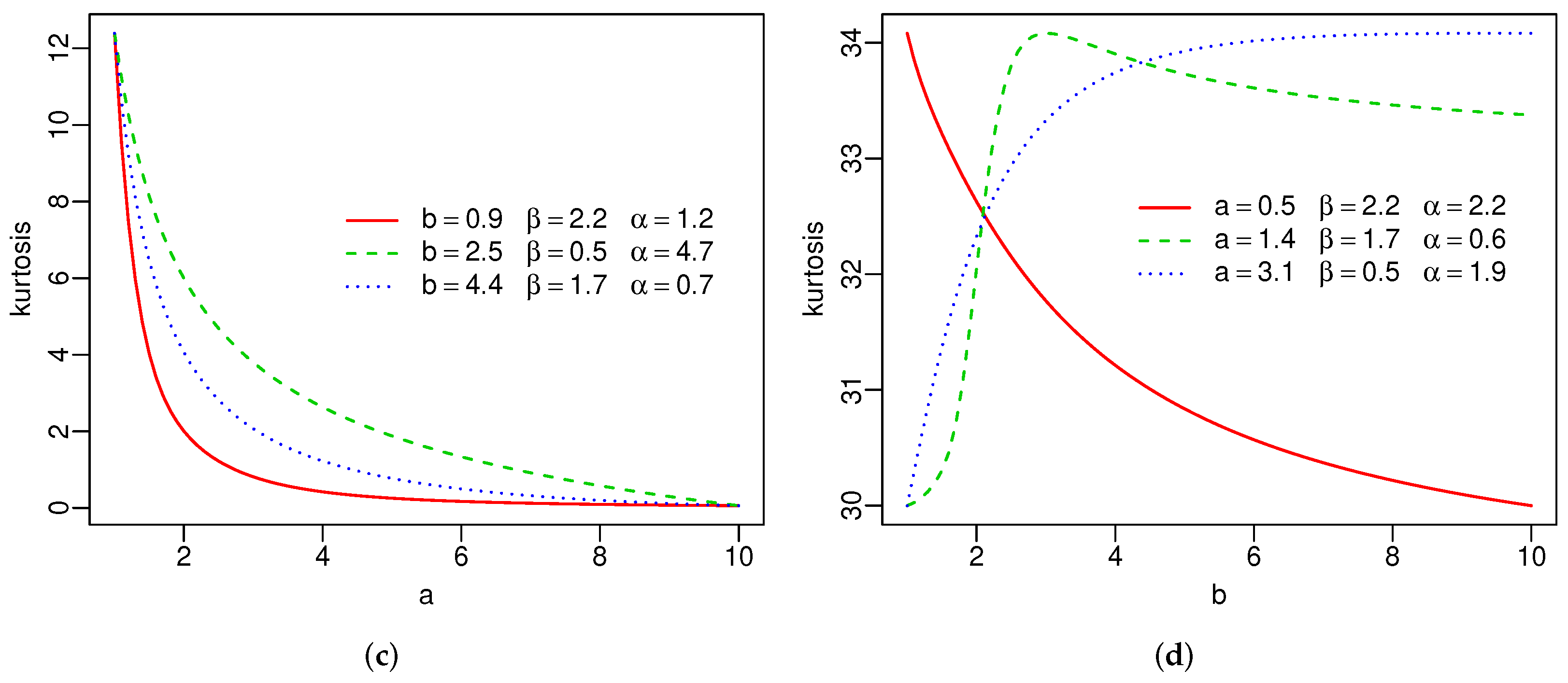
Plots of the skewness and kurtosis of X using R [36] are reported in Figure 3. These measures can be increasing, decreasing, decreasing-increasing, and increasing-decreasing depending on the parameter values.

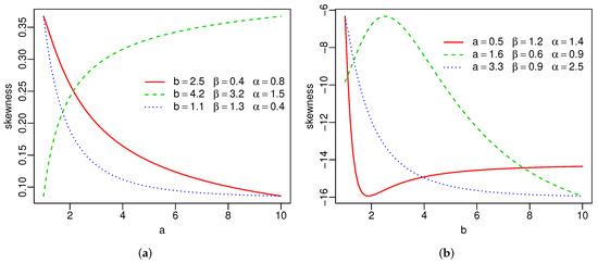
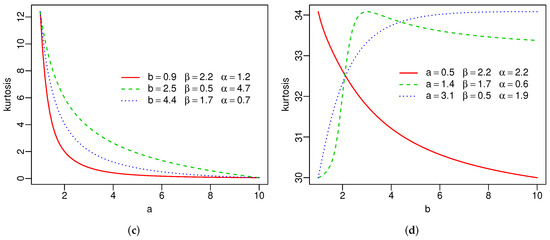
Figure 3. Skewness and kurtosis of the SW$(a,b,\beta ,\alpha )$ distribution(a–d).

5. Estimation

Let $X_i,\cdots ,X_n\sim \mathrm{SG}(a,b,\mathbf{\eta })$ be independent and identically distributed (iid) random variables from (2). The log-likelihood $\ell (a,b,\mathbf{\eta })$ for the parameters from the observed values $x_i,\cdots ,x_n$ has the form

$$\begin{array}{cc}\hfill \ell (a,b,\mathbf{\eta })=& nlogb+\sum _{i=1}^{n}logg(x_i;\mathbf{\eta })+(a-1)\sum _{i=1}^{n}log\{-log[1-G(x_i;\mathbf{\eta })]\}\hfill \\ & -nlog\Gamma (a/b)-\sum _{i=1}^n{\{-log[1-G(x_i;\mathbf{\eta })]\}}^b-\sum _{i=1}^{n}log[1-G(x_i;\mathbf{\eta })].\hfill \end{array}$$

The maximum likelihood estimates (MLEs) can be found by maximizing $\ell (a,b,\mathbf{\eta })$ numerically with respect to the parameters. There are several routines available for the maximization in SAS (PROC NLMIXED), R (optim function), and Ox (sub-routine MaxBFGS).

6. Simulation Study

Consider the SC$(a,b,\lambda ,\beta )$ distribution with sample sizes $n=50$, 100, 150, 200, and 300. We carry out Monte Carlo simulations with 5000 replications to examine the estimation accuracy. The observations are generated from Equation (8), where $Q_{\mathrm{G}}(·)$ is the Chen qf. The true parameters are: $a=0.5$, $b=0.9$, $\lambda =0.4$ and $\beta =1.6$. The simulations were done using the matrix programming language Ox (version 8.02) [37] with the MaxBFGS sub-routine.

The average estimates (AEs), mean square errors (MSEs), and coverage rates of the 95% confidence intervals (CIs) are reported in Table 2. The AEs tend to the true parameters and the MSEs decrease to small values when n increases, thus showing that the estimates are consistent. The simulated CIs are a little greater than 95%.

Table 2. Simulation results from the SC distribution.

n	Parameter	AE	MSE	CI (95%)	Lower (95%)	Upp (95%)
50	a	0.66985	0.17353	97.10	−0.71499	2.05469
	b	1.68281	2.40263	99.84	−4.35142	7.71705
	$\lambda$	0.53627	0.24883	97.22	−1.35293	2.42547
	$\beta$	1.54150	0.57595	97.50	−1.30041	4.38342
100	a	0.60645	0.08474	97.04	−0.26556	1.47846
	b	1.38420	1.34967	99.24	−2.39347	5.16186
	$\lambda$	0.54260	0.19692	97.86	−0.79272	1.87793
	$\beta$	1.56706	0.38844	97.84	−0.52915	3.66326
150	a	0.57948	0.05794	96.72	−0.09699	1.25595
	b	1.25828	0.96073	97.98	−1.63989	4.15645
	$\lambda$	0.53119	0.16704	97.36	−0.50848	1.57086
	$\beta$	1.58631	0.31278	97.98	−0.16239	3.33502
200	a	0.56642	0.04409	96.56	−0.00289	1.13573
	b	1.18037	0.73833	97.20	−1.21682	3.57755
	$\lambda$	0.52359	0.12400	97.66	−0.32081	1.36799
	$\beta$	1.59431	0.27028	98.40	0.06641	3.12220
300	a	0.54599	0.02824	96.44	0.11532	0.97666
	b	1.09099	0.47169	95.08	−0.70170	2.88367
	$\lambda$	0.49700	0.08405	97.52	−0.10430	1.09830
	$\beta$	1.60415	0.20480	98.34	0.34577	2.86254

7. Regression

Consider the random variables X with pdf (3) and $Y=logX$. Setting $s={\mathrm{e}}^{\mu }$ and $c={\sigma }^{-1}$, the density of Y (for $y\in \mathbb{R}$) can be expressed as

$$\begin{array}{cc}\hfill f_{\mathrm{LSBXII}}(y;a,b,\mu ,d,\sigma )=& \frac{b{d}^a}{\sigma \Gamma (a/b)}{\mathrm{e}}^{\frac{y-\mu }{\sigma }}{[1+{\mathrm{e}}^{\frac{y-\mu }{\sigma }}]}^{-1}{\{log[1+{\mathrm{e}}^{\frac{y-\mu }{\sigma }}]\}}^{a-1}\hfill \\ & \times exp\left\{-{\{dlog[1+{\mathrm{e}}^{\frac{y-\mu }{\sigma }}]\}}^b\right\},\hfill \end{array}$$

(9)

where $a,b,d,\sigma >0$ and $\mu \in \mathbb{R}$. Equation (9) has the location-scale form, where $\mu$ is a location and $\sigma$ is a scale. The random variable Y has the log-Stacy-Burr XII (LSBXII) distribution. So, if $X\sim \mathrm{SBXII}(a,b,s,d,c)$, then $Y=logX\sim \mathrm{LSBXII}(a,b,\mu ,d,\sigma )$.

Equation (9) has some special cases. For $b=1$ and $b=d=1$, we have the log-gamma-Burr XII (new) and log-gamma-log-logistic (new), respectively. For $a=b=1$, it is equal to the log-Burr XII (LBXII) density [38]. Finally, the well-know logistic density follows when $a=b=d=1$.

The survival function corresponding to (9) is

$$S_{\mathrm{LSBXII}}(y;a,b,\mu ,d,\sigma )=1-\frac{\gamma ((a/b),{\{dlog[1+{\mathrm{e}}^{\frac{y-\mu }{\sigma }}]\}}^b)}{\Gamma (a/b)}.$$

The density of $Z=(Y-\mu )/\sigma$ (for $z\in \mathbb{R}$) has the form

$$\begin{array}{cc}\hfill f_{\mathrm{LSBXII}}(z;a,b,d)=& \frac{b{d}^a}{\Gamma (a/b)}{\mathrm{e}}^z{\left[1+{\mathrm{e}}^z\right]}^{-1}{\left\{log\left[1+{\mathrm{e}}^z\right]\right\}}^{a-1}\hfill \\ & \times exp\left\{-{\{dlog[1+{\mathrm{e}}^z]\}}^b\right\}.\hfill \end{array}$$

(10)

Equation (10) refers to the standard LSBXII density.

The individuals have different characteristics that make them not identically distributed. For example, in survival analysis, it is common for the failure time to depend on explanatory variables such as fat concentration, blood pressure, glucose level, and sex, among others.

Let ${\mathbf{x}}_i={(x_{i1},\cdots ,x_{ik})}^{\top }$ be the explanatory vector associated with the ith response variable $y_i$ (for $i=1,\dots ,n$), and $\mathbf{\beta }={({\beta }_1,\cdots ,{\beta }_k)}^{\top }$ be the parameter vector. We construct a regression based on the LSBXII distribution

$$y_i={\mathbf{x}}_i^{\top }\mathbf{\beta }+\sigma z_i,i=1,\dots ,n,$$

(11)

where ${\mu }_i={\mathbf{x}}_i^{\top }\mathbf{\beta }$, and $z_i$ is the random error having density function (10).

The density and survival functions of $Y_i$ are

$$\begin{array}{cc}\hfill f_{\mathrm{LSBXII}}(y_i;a,b,d,\sigma ,{\mathbf{\beta }}^{\top })=& \frac{b{d}^a}{\sigma \Gamma (a/b)}{\mathrm{e}}^{z_i}{\left[1+{\mathrm{e}}^{z_i}\right]}^{-1}{\left\{log\left[1+{\mathrm{e}}^{z_i}\right]\right\}}^{a-1}\hfill \\ & \times exp\left\{-{\{dlog[1+{\mathrm{e}}^{z_i}]\}}^b\right\}\hfill \end{array}$$

and

$$S_{\mathrm{LSBXII}}(y_i;a,b,d,\sigma ,{\mathbf{\beta }}^{\top })=1-\frac{\gamma ((a/b),{\{dlog[1+{\mathrm{e}}^{z_i}]\}}^b)}{\Gamma (a/b)},$$

where $z_i=(y_i-{\mathbf{x}}_i^{\top }\mathbf{\beta })/\sigma$. The sets of individuals for which $y_i$ is the log-lifetime or log-censoring are denoted by F and C with r and $n-r$ observations, respectively. Thus, the log-likelihood for $\mathbf{\theta }={(a,b,d,\sigma ,{\mathbf{\beta }}^{\top })}^{\top }$ from model (11) has the form

$$\begin{array}{cc}\hfill \ell \left(\mathbf{\theta }\right)=& rlog\left(\frac{b{d}^a}{\sigma \Gamma (a/b)}\right)+\sum _{i\in F}{z}_i-\sum _{i\in F}log\left[1+{\mathrm{e}}^{z_i}\right]\hfill \\ & +(a-1)\sum _{i\in F}log\left\{log\left[1+{\mathrm{e}}^{z_i}\right]\right\}-\sum _{i\in F}{\{dlog[1+{\mathrm{e}}^{z_i}]\}}^b\hfill \\ & +\sum _{i\in C}log\left\{1-\frac{\gamma ((a/b),{\{dlog[1+{\mathrm{e}}^{z_i}]\}}^b)}{\Gamma (a/b)}\right\}.\hfill \end{array}$$

(12)

For $r=n$, $y_i\in F$ ($\forall i$), the log-likelihood (12) reduces to the usual log-likelihood. The MLE $\widehat{\mathbf{\theta }}$ can be found by maximizing (12) numerically using the optim function of R [36].

We assume that the asymptotic likelihood theory holds, i.e., $(\widehat{\mathbf{\theta }}-\mathbf{\theta })\stackrel{a}{\sim }{\mathcal{N}}_{k+4}(\mathbf{0},{\mathbf{J}}^{-1}\left(\mathbf{\theta }\right))$, where $\stackrel{a}{\sim }$ denotes asymptotic distribution and $\mathbf{J}\left(\mathbf{\theta }\right)$ is the observed information matrix for the model parameters.

8. Applications

We prove the potentiality of the proposed models by means of three applications, as well as the utility of the proposed models by means of three applications (Appendix A). We apply the SBXII distribution to two uncensored data in the first two, and we fit the LSBXII regression to censored data in the third one.

8.1. Uncensored Data

The uncensored data sets are:

(1)

The first data set consists of the sum of skin folds in 202 athletes collected at the Australian Institute of Sports (skin folds data). These data were also analyzed by [39];

(2)

The second data set ($n=40$), discussed by [40] and [22], refers to the time-to-failure (${10}^3$ h) of a particular type of engine (turbocharger data).

We fit five distributions: SBXII (3), gamma-Burr XII [31], beta-Burr XII (BBXII) [41], Kumaraswamy–Burr XII (KBXII) [42], and Weibull–Burr XII [43] to both data sets.

The BBXII and KBXII densities are (for $x>0$)

$$\begin{array}{cc}\hfill f_{\mathrm{BBXII}}(x;a,b,s,d,c)=& \frac{cd}{s^{c}B(a,b)}{x}^{c-1}{[1+{(x/s)}^c]}^{-(db+1)}\hfill \\ \hfill & \times {\left\{1-{[1+{(x/s)}^c]}^{-d}\right\}}^{a-1}\hfill \end{array}$$

and

$$\begin{array}{cc}\hfill f_{\mathrm{KBXII}}(x;a,b,s,d,c)=& abcd{s}^{-c}{x}^{c-1}{[1+{(x/s)}^c]}^{-(d+1)}{\left\{1-{[1+{(x/s)}^c]}^{-d}\right\}}^{a-1}\hfill \\ & \times {\{1-{\{1-{[1+{(x/s)}^c]}^{-d}\}}^a\}}^{b-1},\hfill \end{array}$$

respectively, where all parameters are positive.

The Weibull–Burr XII (WBXII) density introduced by [43] (taking the scale parameter $s=1$) is (for $x>0$)

$$\begin{array}{cc}\hfill f_{\mathrm{WBXII}}(x;a,b,d,c)=& abcd{x}^{c-1}{(1+x^c)}^{bd-1}{[1-{(1+x^c)}^{-d}]}^{b-1}\hfill \\ \hfill & \times exp\{-a{[{(1+x^c)}^d-1]}^b\},\hfill \end{array}$$

where all parameters are positive.

The MLEs for all models are calculated using the optim function (with BFGS method) available in R [36]. We adopt the Cramér-von Mises ($W^{*}$) and Anderson-Darling ($A^{*}$) measures [44] for model comparisions. The MLEs and their standard errors (SEs) in parentheses and the information criteria are reported in Table 3 and Table 4 for both data sets, where the statistics $W^{*}$ and $A^{*}$ reveal that the SBXII distribution provides the best fit followed by the KBXII distribution in the first case, and by the GBXII distribution in the second case.

Table 3. Results from the fitted models to skin folds data.

Distribution	a	b	s	d	c
BXII	-	-	47.3209	0.4885	5.2992
	-	-	(5.8102)	(0.1909)	(1.1667)
GBXII	6.7710	-	19.1049	0.4019	14.2138
	(4.3046)	-	(6.3462)	(0.3117)	(9.9266)
SBXII	1.1357	4.4497	29.7613	0.0307	22.6525
	(0.1854)	(1.1481)	(1.3755)	(0.0090)	(6.3063)
BBXII	8.7445	9.0397	16.8470	0.0671	8.0123
	(6.7799)	(10.2228)	(7.4968)	(0.0684)	(6.9791)
KBXII	2.5656	21.4299	24.8132	0.0181	18.9969
	(0.6304)	(9.2078)	(2.9297)	(0.0054)	(5.2688)
WBXII	0.4688	6.9807	-	0.1133	1.5193
	(0.2857)	(0.3949)	-	(0.0197)	(0.2571)
Distribution	${\mathit{W}}^{*}$	${\mathit{A}}^{*}$
BXII	0.2803	1.8868
GBXII	0.1564	1.1153
SBXII	0.0670	0.4116
BBXII	0.1602	1.1205
KBXII	0.1325	0.9377
WBXII	0.5443	3.1913

Table 4. Results from the fitted models to the turbocharger data.

Distribution	a	b	s	d	c
BXII	-	-	17.4122	36.2491	3.8786
	-	-	(7.1825)	(52.4338)	(0.5282)
GBXII	0.1577	-	10.0683	8.9154	16.3307
	(0.0267)	-	(0.0435)	(3.9008)	(0.0435)
SBXII	0.1559	25.0319	9.3438	2.1176	15.3057
	(0.0249)	(59.5089)	(0.2099)	(0.6168)	(0.2090)
BBXII	0.1676	9.0200	10.7368	2.5707	15.5021
	(0.0284)	(3.8937)	(0.0555)	(0.0309)	(0.0622)
KBXII	0.3557	14.1922	18.0505	10.1027	10.3163
	(0.0534)	(9.6999)	(1.0707)	(15.5092)	(0.5361)
WBXII	0.0099	6.5239	-	0.7123	0.6825
	(0.0109)	(3.3203)	-	(0.1775)	(0.4227)
Distribution	${\mathit{W}}^{*}$	${\mathit{A}}^{*}$
BXII	0.0796	0.5913
GBXII	0.0153	0.1220
SBXII	0.0114	0.0866
BBXII	0.0154	0.1222
KBXII	0.0693	0.5228
WBXII	0.0830	0.6136

The likelihood ratio (LR) test can be sed for the sub-models GBXII and BXII of the SBXII distribution for $a=1$ and $a=b=1$, respectively. Table 5 reports the LR tests for both datasets. Except for SBXII vs. GBXII in the turbocharger data, which is at the 10% significance threshold, all LR tests are highly significant. Then, the SBXII model fits the data better than its sub-models.

Table 5. LR tests for skin folds and turbocharger data.

Model	Hypotheses	LR	p-Value
skin folds data
GBXII vs. SBXII	${\mathcal{H}}_0$:$b=1$ vs. ${\mathcal{H}}_1$: ${\mathcal{H}}_0$ is false	15.4902	0.0001
BXII vs. SBXII	${\mathcal{H}}_0$:$a=b=1$ vs. ${\mathcal{H}}_1$: ${\mathcal{H}}_0$ is false	33.7721	<0.0001
turbocharger data
GBXII vs. SBXII	${\mathcal{H}}_0$:$b=1$ vs. ${\mathcal{H}}_1$: ${\mathcal{H}}_0$ is false	2.6189	0.1056
BXII vs. SBXII	${\mathcal{H}}_0$:$a=b=1$ vs. ${\mathcal{H}}_1$: ${\mathcal{H}}_0$ is false	10.8621	0.0044

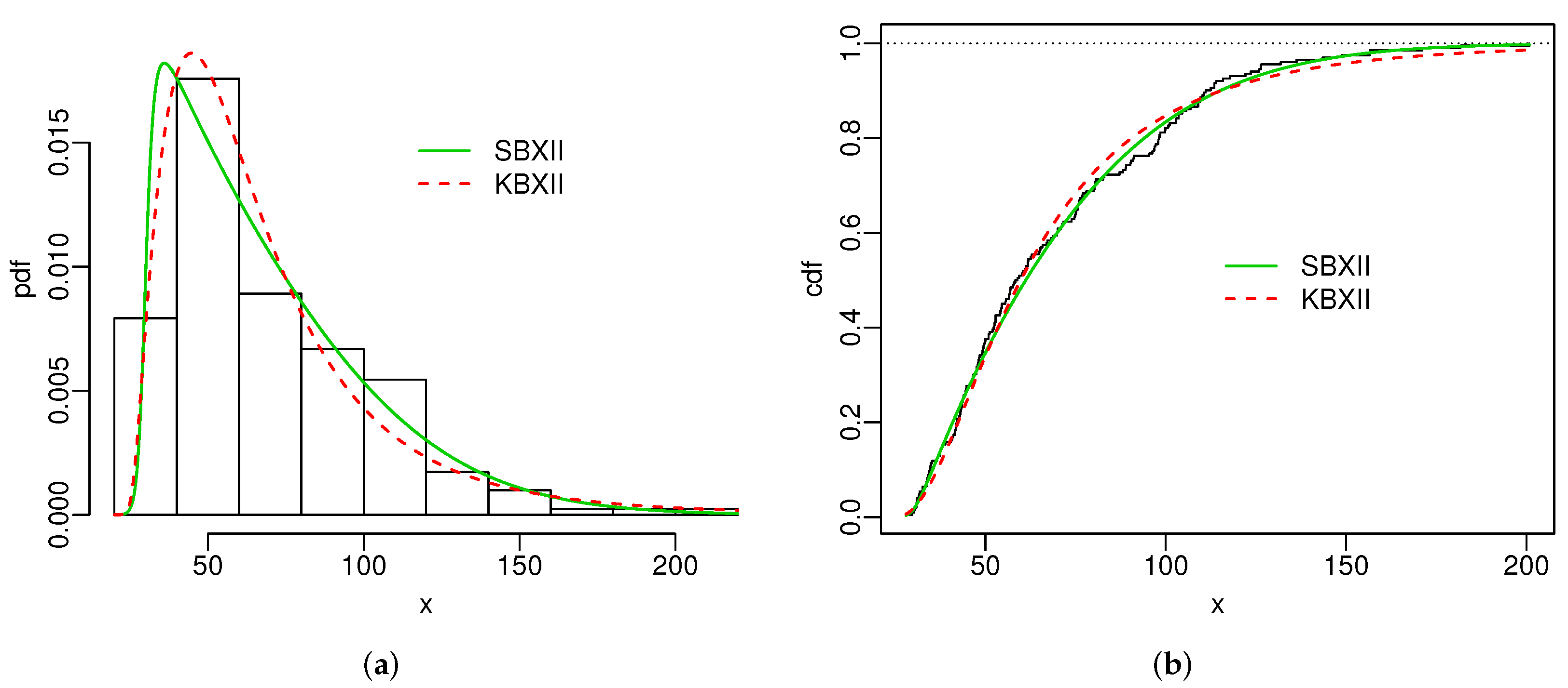
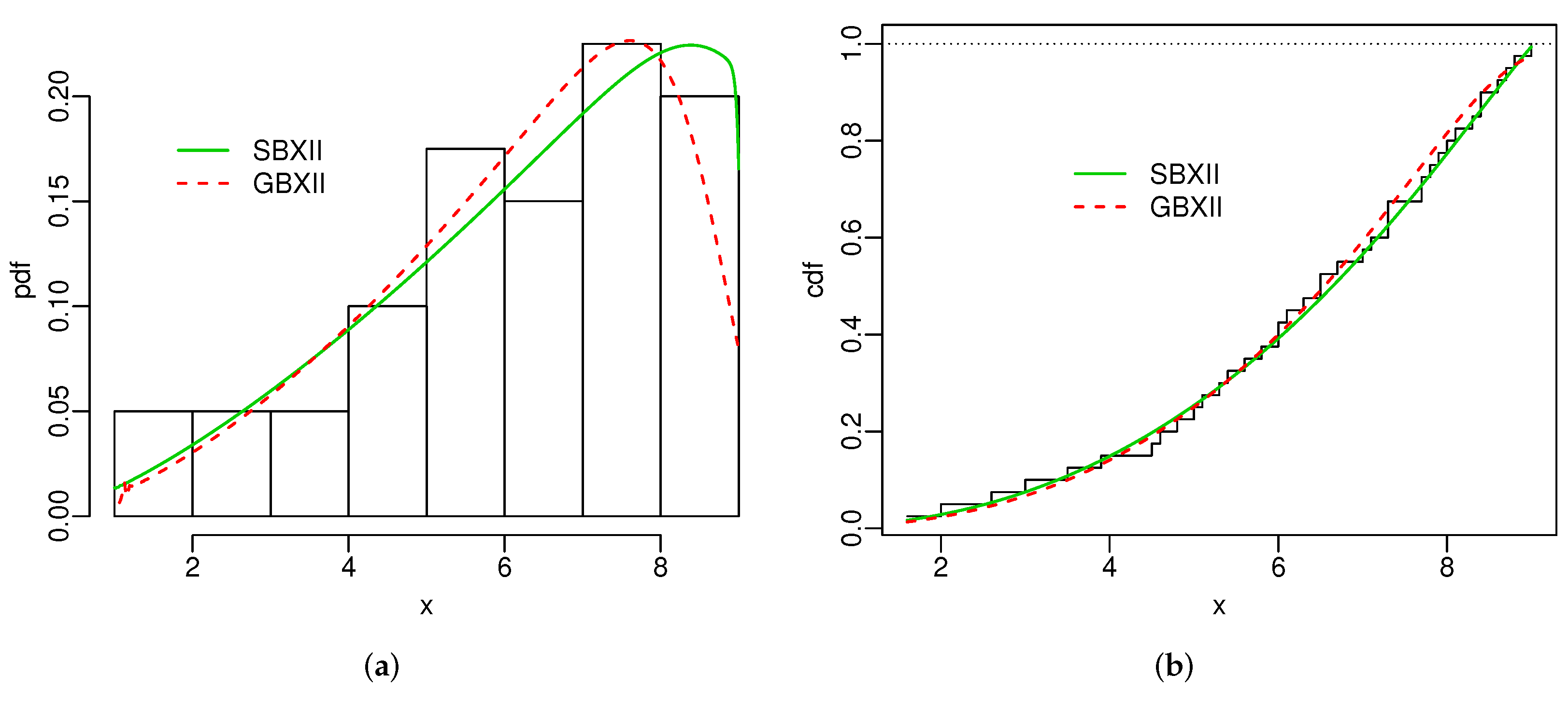
Figure 4 and Figure 5 display the histogram and Kaplan-Meier empirical cdf in conjunction with the best estimated pdfs and cdfs for both datasets. The superiority of the SBXII model is supported by the statistics $W^{*}$ and $A^{*}$.

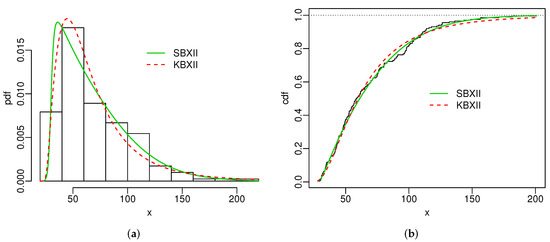
Figure 4. Estimated pdfs (a) and estimated cdfs (b) for skin folds data.

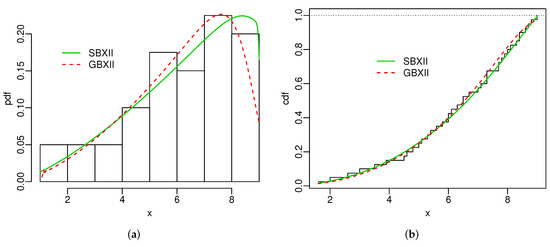
Figure 5. Estimated pdfs (a) and estimated cdfs (b) for turbocharger data.

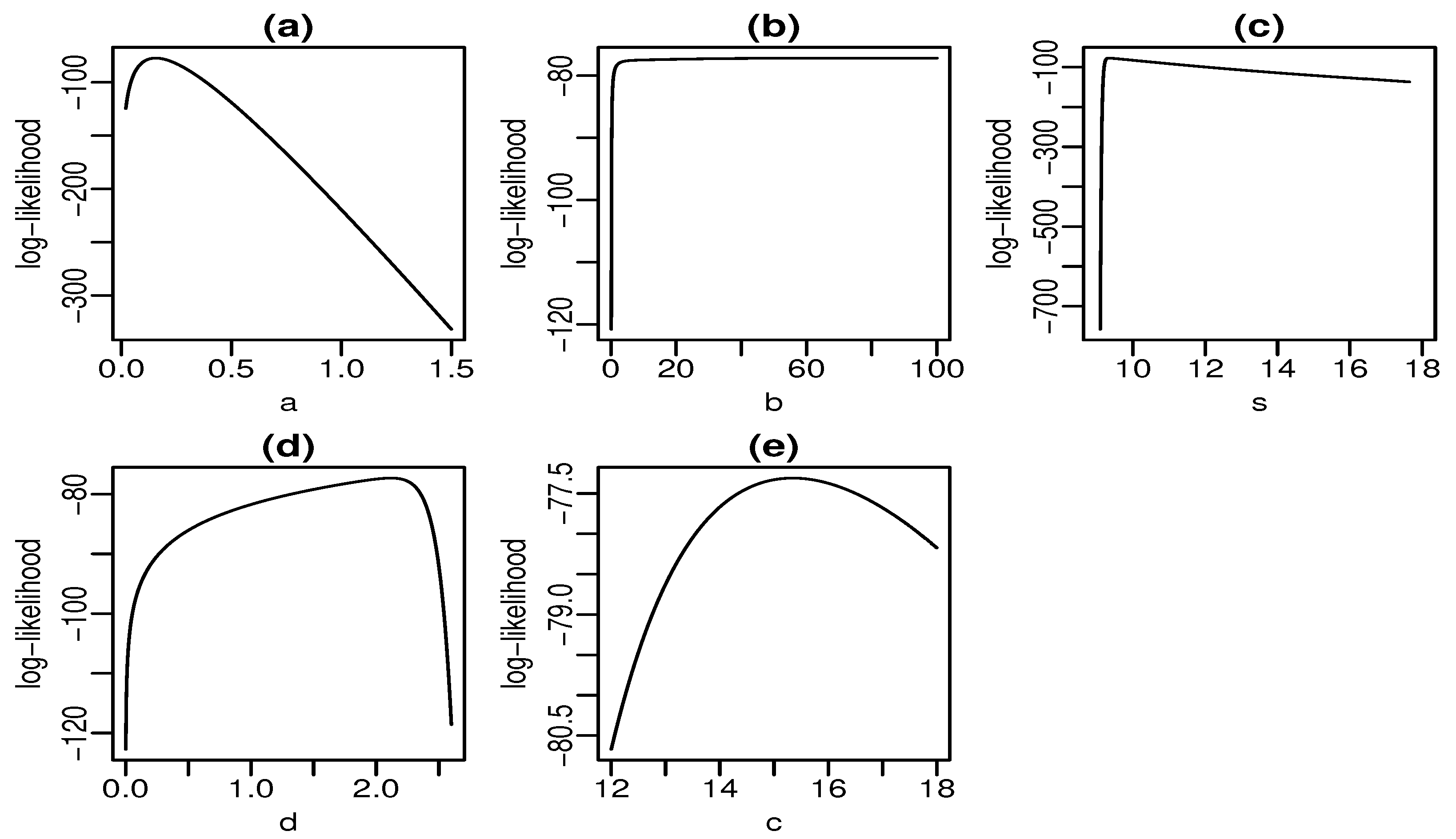
Figure 6 and Figure 7 display plots of the profile log-likelihood function versus some parameter values (the MLEs of the other parameters fixed) for the skin folds and turbocharger data, respectively. We can find the approximate intervals that maximize the profile log-likelihood function for each parameter. In Figure 6a, the log-likelihood is maximized for values of a close to one. Similarly, it takes maximum values for $0<b<10$, $15<s<50$, $0.0014<d<0.05$, and $0<c<40$ according to Figure 6b–e, respectively. The interpretation from Figure 7 is analogous. Nevertheless, there is evidence of a monotone log-likelihood in Figure 7b since this function does not have a maximum in the range taken for b.

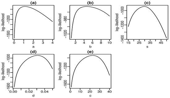
Figure 6. Profile log-likelihood functions for skin folds data (a–e).

Figure 7. Profile log-likelihood functions for turbocharger data (a–e).

8.2. Regression for Censored Data

We apply the LSBXII regression addressed in Section 7 to the recurrence times (in years) of 417 patients with melanoma cancer under the effect of a high dose of a drug (interferon alfa-2b) [45]. The study was conducted from 1991 to 1995, and the patients were followed up until 1998 under right censoring (0 = censoring and 1 = observed lifetime). The percentage of censoring is 55.64%. The explanatory variable $x_{i1}$ (nodule category) denotes the number of lymph nodes involved in the disease (0, 1, 2–3, and ≥4). The proposed regression is

$$y_i={\beta }_0+{\beta }_1{x}_{i1}+\sigma z_i,i=1,\dots ,417,$$

where $z_i$ has density (10). Table 6 gives the MLEs, their SEs in parentheses, and p-values in brackets for the LSBXII regression and two sub-models fitted to these data. The estimates are statistically significant at 1% for the three models, thus showing that $x_1$ affects the lifetime. The negative sign of ${\beta }_1$ indicates that the higher the degree of the nodule, the shorter the failure time.

Table 6. MLEs, SEs, and p-values for three regression.

Model	a	b	d	$\mathit{\sigma }$	${\mathit{\beta }}_0$	${\mathit{\beta }}_1$
LSBXII	0.5636	0.1939	5.6590	0.1807	1.9576	−0.2568
	(0.1664)	(0.0463)	(15.4211)	(0.0289)	(0.2748)	(0.0580)
	[0.0007]	[0.0000]	[0.7136]	[0.0000]	[0.0000]	[0.0000]
LBXII	-	-	0.0159	0.0999	0.8932	−0.2148
	-	-	(0.0058)	(0.0342)	(0.1919)	(0.0690)
	-	-	[0.0058]	[0.0035]	[0.0000]	[0.0018]
Logistic	-	-	-	1.8247	6.5851	−0.8718
	-	-	-	(0.1129)	(0.4623)	(0.1630)
	-	-	-	[0.0000]	[0.0000]	[0.0000]

Table 7 gives the classical statistics CAIC, AIC, BIC, and HQIC for three regressions, which reveal that the LSBXII regression is the best model for these data.

Table 7. Adequacy measures for three regressions.

Model	CAIC	AIC	BIC	HQIC
LSBXII	1055.9662	1055.7613	1079.9598	1065.3284
LBXII	1079.4012	1079.3042	1095.4365	1085.6822
Logistic	1243.0194	1242.9613	1255.0606	1247.7449

The LR statistics comparing the LSBXII regression with two sub-models in Table 8 also support that the LSBXII model is the best model among the three.

Table 8. LR tests for three regressions.

Model	Hyphotheses	LR	p-Value
LBXII vs. LSBXII	${\mathcal{H}}_0$:$a=b=1$ vs. ${\mathcal{H}}_1$: ${\mathcal{H}}_0$ is false	13.7714	<0.0001
Logistic vs. LSBXII	${\mathcal{H}}_0$:$a=b=d=1$ vs. ${\mathcal{H}}_1$: ${\mathcal{H}}_0$ is false	96.6000	<0.0001

9. Conclusions

We defined a new Stacy-G class of distributions, which extends the gamma-G family [30], and proved its flexibility. Some of its mathematical properties were presented. A simulation study showed the consistency of the maximum likelihood estimators. We constructed a new log-Stacy-Burr XII regression for censored data. Three applications to real data using the Burr XII baseline revealed the utility of the proposed models when compared to other models.

Appendix A.1. Figures Codes

# Stacy Burr XII

# pdf

pdf.SBXII <- function(par, x) {

a <- par[1]

b <- par[2]

s <- par[3]

d <- par[4]

c <- par[5]

f1 <- b*c*d^a/(s^c*gamma(a/b)) * x^(c-1) * (1+(x/s)^c)^(-1)

f2 <- log(1+(x/s)^c)^(a-1) * exp(-(d*log((1+(x/s)^c)))^b)

fd <- f1 * f2

fd

}

# cdf

cdf.SBXII <- function(par, x) {

a <- par[1]

b <- par[2]

s <- par[3]

d <- par[4]

c <- par[5]

fa <- pgamma((d*log(1+(x/s)^c))^b, a/b)

fa

}

# hrf

hrf.SBXII <- function(par, x) {

a <- par[1]

b <- par[2]

s <- par[3]

d <- par[4]

c <- par[5]

fd <- b*c*d^a/(s^c*gamma(a/b)) * x^(c-1) * (1+(x/s)^c)^(-d-1) *

log(1+(x/s)^c)^(a-1) * exp(-(d*log((1+(x/s)^c)))^b) * (1+(x/s)^c)^d

fa <- pgamma((d*log(1+(x/s)^c))^b, a/b)

hr <- fd / (1-fa)

hr

}

# Stacy Uniform

# pdf

pdf.SUnif <- function(par, x){

a <- par[1]

b <- par[2]

c<- par[3]

d <- par[4]

G <- punif(x, c, d)

g <- dunif(x, c, d)

fd <- b/(gamma(a/b)*(d-x)) * (-log((d-x)/(d-c)))^(a-1) * exp(-(-log((d-x)/(d-c)))^b)

fd

}

# cdf

cdf.SUnif <- function(par, x){

a <- par[1]

b <- par[2]

c <- par[3]

d <- par[4]

fa <- pgamma((-log((d-x)/(d-c)))^b, a/b)

fa

}

################

# Stacy-Chen

# pdf

pdf.SC <- function(par, x){

a <- par[1]

b <- par[2]

lambda <- par[3]

beta <- par[4]

b*lambda^a*beta/gamma(a/b)*x^(beta-1) * (exp(x^beta)-1)^(a-1) *

exp(x^beta - (-lambda*(1-exp(x^beta)))^b )

}

# cdf

cdf.SC <- function(par, x){

a <- par[1]

b <- par[2]

lambda <- par[3]

beta <- par[4]

pgamma((-lambda*(1-exp(x^beta)))^b, a/b)

}

# hrf

hrf.SC <- function(par, x){

a <- par[1]

b <- par[2]

lambda <- par[3]

beta <- par[4]

fd = b*lambda^a*beta/gamma(a/b)*x^(beta-1) * (exp(x^beta)-1)^(a-1) *

exp(x^beta - (-lambda*(1-exp(x^beta)))^b )

fa = pgamma((-lambda*(1-exp(x^beta)))^b, a/b)

fd / (1-fa)

}

# Stacy Weibull

# fdp

pdf.SW <- function(par, x){

a <- par[1]

b <- par[2]

beta <- par[3]

alpha <- par[4]

fd <- b*alpha*beta^(a*alpha)/gamma(a/b) * x^(a*alpha-1) * exp(-(beta*x)^(b*alpha))

fd

}

# cdf

cdf.SW <- function(par, x){

a <- par[1]

b <- par[2]

beta <- par[3]

alpha <- par[4]

fa <- pgamma((beta*x)^(b*alpha), a/b)

fa

}

# hrf

hrf.SW <- function(par, x){

a <- par[1]

b <- par[2]

beta <- par[3]

alpha <- par[4]

fd <- b*alpha*beta^(a*alpha)/gamma(a/b) * x^(a*alpha-1) * exp(-(beta*x)^(b*alpha))

fa <- pgamma((beta*x)^(alpha*b), a/b)

hr <- fd / (1-fa)

hr

}

## density curves

par(mfrow=c(1,1))

par(mar=c(2.8, 2.8, .5, .5))

par(mgp=c(1.6, 0.45, 0))

# SBXII

{

curve(pdf.SBXII(c(2.7,2.2,1.2,.7,2.5),x), xlim = c(0,5), col=1, n=2000, ylab = "pdf", lwd=1.5, lty=1)

par(new=T)

curve(pdf.SBXII(c(.4,2,1.2,.7,2.5),x), xlim = c(0,4), col=2, n=2000, axes=F,ann=F, lwd=1.5, lty=2)

par(new=T)

curve(pdf.SBXII(c(3.8,.7,1.2,.7,2.5),x), xlim = c(0,58), col=3, n=2000, axes=F,ann=F, lwd=1.5, lty=3)

par(new=T)

curve(pdf.SBXII(c(1.5,.2,1.2,.7,2.5),x), xlim = c(0,10), col=4, n=2000, axes=F,ann=F, lwd=1.5, lty=4)

par(new=T)

curve(pdf.SBXII(c(.8,1.5,1.2,.7,2.5),x), xlim = c(0,8), col=5, n=2000, axes=F,ann=F, lwd=1.5, lty=5)

legend("topright", legend = c(expression(paste(a==2.7," ", " ", " ", b==2.2)),

expression(paste(a==.4," ", " ", " ", b==2)),

expression(paste(a==3.8," ", " ", " ", b==.7)),

expression(paste(a==1.5," ", " ", " ", b==.2)),

expression(paste(a==.8," ", " ", " ", b==1.5))),

lwd=1.5, bty = "n", col = 1:5, lty=1:5)

}

# SUnif

{

curve(pdf.SUnif(c(2.1,3.7,0,8),x), xlim = c(0,8), col=1, n=2000, ylab = "pdf", lwd=1.5, lty=1)

par(new=T)

curve(pdf.SUnif(c(.9,2.9,0,8),x), xlim = c(0,8), col=2, n=2000, axes=F,ann=F, lwd=1.5, lty=2)

par(new=T)

curve(pdf.SUnif(c(.8,1.1,0,8),x), xlim = c(0,8), col=3, n=2000, axes=F,ann=F, lwd=1.5, lty=3)

par(new=T)

curve(pdf.SUnif(c(1.6,1.6,0,8),x), xlim = c(0,8), col=4, n=2000, axes=F,ann=F, lwd=1.5, lty=4)

par(new=T)

curve(pdf.SUnif(c(1.1,.9,0,8),x), xlim = c(0,8), col=5, n=2000, axes=F,ann=F, lwd=1.5, lty=5)

legend(.2,.64, legend = c(expression(paste(a==2.1," ", " ", " ", b==3.7)),

expression(paste(a==.9," ", " ", " ", b==2.9)),

expression(paste(a==.8," ", " ", " ", b==1.1)),

expression(paste(a==1.6," ", " ", " ", b==1.6)),

expression(paste(a==1.1," ", " ", " ", b==.9))),

lwd=1.5, bty = "n", col=1:5, lty=1:5)

}

# SC

{

curve(pdf.SC(c(.6,.2,1.7,1.3),x), xlim = c(0,9), col=1, n=2000, ylab = "pdf", lwd=1.5, lty=1)

par(new=T)

curve(pdf.SC(c(1.6,.4,1.7,1.3),x), xlim = c(0,15), col=2, n=2000, axes=F,ann=F, lwd=1.5, lty=2)

par(new=T)

curve(pdf.SC(c(.3,.1,1.7,1.3),x), xlim = c(0,15), col=3, n=2000, axes=F,ann=F, lwd=1.5, lty=3)

par(new=T)

curve(pdf.SC(c(.6,1.2,1.7,1.3),x), xlim = c(0,5), col=4, n=2000, axes=F,ann=F, lwd=1.5, lty=4)

par(new=T)

curve(pdf.SC(c(2.1,.2,1.7,1.3),x), xlim = c(0,15), col=5, n=2000, axes=F,ann=F, lwd=1.5, lty=5)

legend("topright", legend = c(expression(paste(a==.6," ", " ", " ", b==.2)),

expression(paste(a==1.6," ", " ", " ", b==.4)),

expression(paste(a==.3," ", " ", " ", b==.1)),

expression(paste(a==.6," ", " ", " ", b==1.2)),

expression(paste(a==2.1," ", " ", " ", b==.2))),

lwd=1.5, bty = "n", col=1:5, lty=1:5)

}

# SW

{

curve(pdf.SW(c(1.2,1.2,.5,1.7),x), xlim = c(0,12), col=1, n=2000, ylab = "pdf", lwd=1.5, lty=1)

par(new=T)

curve(pdf.SW(c(3.2,.6,.5,1.7),x), xlim = c(0,15), col=2, n=2000, axes=F,ann=F, lwd=1.5, lty=2)

par(new=T)

curve(pdf.SW(c(2.2,.8,.5,1.7),x), xlim = c(0,12), col=3, n=2000, axes=F,ann=F, lwd=1.5, lty=3)

par(new=T)

curve(pdf.SW(c(.9,.4,.5,1.7),x), xlim = c(0,12), col=4, n=2000, axes=F,ann=F, lwd=1.5, lty=4)

par(new=T)

curve(pdf.SW(c(.5,2.5,.5,1.7),x), xlim = c(0,5), col=5, n=2000, axes=F,ann=F, lwd=1.5, lty=5)

legend(2.8,1.1, legend = c(expression(paste(a==1.2," ", " ", " ", b==1.2)),

expression(paste(a==3.2," ", " ", " ", b==.6)),

expression(paste(a==2.2," ", " ", " ", b==.8)),

expression(paste(a==.9," ", " ", " ", b==.4)),

expression(paste(a==.5," ", " ", " ", b==2.5))),

lwd=1.5, bty = "n", col=1:5, lty=1:5)

}

# hrfs curves

# SBXII

{

curve(hrf.SBXII(c(.3,.4,1.9,.4,2.2),x), xlim = c(0,12), col=1, n=200, ylab = "pdf", lwd=1.5, lty=1)

par(new=T)

curve(hrf.SBXII(c(.1,4.5,1.9,.4,2.2),x), xlim = c(0,12), col=2, n=200, axes=F,ann=F, lwd=1.5, lty=2)

par(new=T)

curve(hrf.SBXII(c(.8,1.3,1.9,.4,2.2),x), xlim = c(0,12), col=3, n=200, axes=F,ann=F, lwd=1.5, lty=3)

par(new=T)

curve(hrf.SBXII(c(3.4,3.7,1.9,.4,2.2),x), xlim = c(0,12), col=4, n=200, axes=F,ann=F, lwd=1.5, lty=4)

legend(.75,.74, legend = c(expression(paste(a==.3," ", " ", " ", b==.4)),

expression(paste(a==.1," ", " ", " ", b==4.5)),

expression(paste(a==.8," ", " ", " ", b==1.3)),

expression(paste(a==3.4," ", " ", " ", b==3.7))),

lwd=1.5, bty = "n", col=1:4, lty=1:4 )

}

# SW

{

curve(hrf.SW(c(.6,.4,.7,1.5),x), xlim = c(0,8), col=1, n=200, ylab = "pdf", lwd=1.5, lty=1)

par(new=T)

curve(hrf.SW(c(.8,.9,.7,1.5),x), xlim = c(0,8), col=2, n=200, axes=F,ann=F, lwd=1.5, lty=2)

par(new=T)

curve(hrf.SW(c(.1,1.1,.7,1.5),x), xlim = c(0,8), col=3, n=200, axes=F,ann=F, lwd=1.5, lty=3)

par(new=T)

curve(hrf.SW(c(.9,.3,.7,1.5),x), xlim = c(0,8), col=4, n=200, axes=F,ann=F, lwd=1.5, lty=4)

#par(new=T)

#curve(hrf.SW(c(.6,.4,.7,1.5),x), xlim = c(0,8), col=7, n=200, axes=F,ann=F)

legend(.6,.061, legend = c(expression(paste(a==.6," ", " ", " ", b==.4)),

expression(paste(a==.8," ", " ", " ", b==.9)),

expression(paste(a==.1," ", " ", " ", b==1.1)),

expression(paste(a==.9," ", " ", " ", b==.3))),

lwd=1.5, bty = "n", col=1:4, lty=1:4)

}

#################################################################################

######################    Assimetria e kurtose da SW   #####################

#################################################################################

# momentos centrais

# UWW distribution

momcentral_SW <- function(param, r){

mu1 <- pdf.SW <- function(x, par=param){

a <- par[1]

b <- par[2]

beta <- par[3]

alpha <- par[4]

fd <- b*alpha*beta^(a*alpha)/gamma(a/b) * x^(a*alpha-1) * exp(-(beta*x)^(b*alpha))

fd

}

meanx <- integrate(mu1, 0, Inf, subdivisions = 1e6)$value

mu2.central <- function(x, par=param, mu=meanx){

a <- par[1]

b <- par[2]

beta <- par[3]

alpha <- par[4]

fd1 <- b*alpha*beta^(a*alpha)/gamma(a/b) * x^(a*alpha) * exp(-(beta*x)^(b*alpha))

fd <- fd1 * (x-mu)^2

fd

}

mur.central <- function(x, par=param, mu=meanx,k=r){

a <- par[1]

b <- par[2]

beta <- par[3]

alpha <- par[4]

fd1 <- b*alpha*beta^(a*alpha)/gamma(a/b) * x^(a*alpha-1) * exp(-(beta*x)^(b*alpha))

fd <- fd1 * (x-mu)^k

fd

}

mom2_central <-  integrate(mu2.central, 0, Inf, subdivisions = 1e6)$value

momr_central <-  integrate(mur.central, 0, Inf, subdivisions = 1e6)$value

# padronizando

mom_central_Padr <-  momr_central / mom2_central^(r/2)

mom_central_Padr

#list(mu=meanx)

}

momcentral_SW(c(2,1.4,.2,1.4),0)

momcentral_SW(c(.9,1.4,4.2,.4),0)

a <- seq(from=1,by=.02, to=10)

b <- seq(from=1,by=.02, to=10)

a <- seq(from=1,by=.1, to=10)

b <- seq(from=1,by=.1, to=10)

# assimetria

assimetria_a <- vector()

assimetria_a2 <- vector()

assimetria_a3 <- vector()

assimetria_b <- vector()

assimetria_b2 <- vector()

assimetria_b3 <- vector()

for (i in 1:length(a)) {

print(i)

assimetria_a[i] <- momcentral_SW(c(a[i], 2.5, .4, .8), 3)

assimetria_a2[i] <- momcentral_SW(c(a[i], 4.2, 3.2, 1.5), 3)

assimetria_a3[i] <- momcentral_SW(c(a[i], 1.1, 1.3, .4), 3)

assimetria_b[i] <- momcentral_SW(c(.5, b[i], 1.2, 1.4), 3)

assimetria_b2[i] <- momcentral_SW(c(1.6, b[i], .6, .9), 3)

assimetria_b3[i] <- momcentral_SW(c(3.3, b[i], 2.9, 2.5), 3)

}

# curvas

# para a

{

plot(a,assimetria_a, type = "l", ylab = "skewness", col=2, lwd=1.5, lty=1)

par(new=T)

plot(a,assimetria_a2, type = "l", ylab = "skewness", col=3, axes = F, ann = F, lwd=1.5, lty=2)

par(new=T)

plot(a,assimetria_a3, type = "l", ylab = "skewness", col=4, axes = F, ann = F, lwd=1.5, lty=3)

legend(4.5,.02, legend = c(

expression(paste(b==2.5, " ", " ", " ", beta==.4, " ", " ", " ", alpha==.8)),

expression(paste(b==4.2, " ", " ", " ", beta==3.2, " ", " ", " ", alpha==1.5)),

expression(paste(b==1.1, " ", " ", " ", beta==1.3, " ", " ", " ", alpha==.4))

),

bty = "n", col = 2:4, lwd=1.5, lty=1:3)

}

# para b

{

plot(b,assimetria_b, type = "l", ylab = "skewness", col=2, lwd=1.5, lty=1)

par(new=T)

plot(b,assimetria_b2, type = "l", ylab = "skewness", col=3, axes = F, ann = F, lwd=1.5, lty=2)

par(new=T)

plot(b,assimetria_b3, type = "l", ylab = "skewness", col=4, axes = F, ann = F, lwd=1.5, lty=3)

legend(4.4,-3.5, legend = c(

expression(paste(a==.5, " ", " ", " ", beta==1.2, " ", " ", " ", alpha==1.4)),

expression(paste(a==1.6, " ", " ", " ", beta==.6, " ", " ", " ", alpha==.9)),

expression(paste(a==3.3, " ", " ", " ", beta==.9, " ", " ", " ", alpha==2.5))

),

bty = "n", col = 2:4, lwd=1.5, lty=1:3)

}

# kurtose

kurtose_a <- vector()

kurtose_a2 <- vector()

kurtose_a3 <- vector()

kurtose_b <- vector()

kurtose_b2 <- vector()

kurtose_b3 <- vector()

for (i in 1:length(a)) {

print(i)

kurtose_a[i] <- momcentral_SW(c(a[i], .9, 2.2, 1.2), 4)

kurtose_a2[i] <- momcentral_SW(c(a[i], 2.5, .5, 4.7), 4)

kurtose_a3[i] <- momcentral_SW(c(a[i], 4.4, 1.7, .7), 4)

kurtose_b[i] <- momcentral_SW(c(.5, b[i], 2.2, 2.2), 4)

kurtose_b2[i] <- momcentral_SW(c(1.4, b[i], 1.7, .6), 4)

kurtose_b3[i] <- momcentral_SW(c(3.1, b[i], .5, 1.9), 4)

}

# curvas

# para a

{

plot(a,kurtose_a, type = "l", ylab = "kurtosis", col=2, lwd=1.5, lty=1)

par(new=T)

plot(a,kurtose_a2, type = "l", ylab = "kurtosis", col=3, axes = F, ann = F, lwd=1.5, lty=2)

par(new=T)

plot(a,kurtose_a3, type = "l", ylab = "kurtosis", col=4, axes = F, ann = F, lwd=1.5, lty=3)

legend(4,36, legend = c(

expression(paste(b==.9, " ", " ", " ", beta==2.2, " ", " ", " ", alpha==1.2)),

expression(paste(b==2.5, " ", " ", " ", beta==.5, " ", " ", " ", alpha==4.7)),

expression(paste(b==4.4, " ", " ", " ", beta==1.7, " ", " ", " ", alpha==.7))

),

bty = "n", col = 2:4, lwd=1.5, lty=1:3)

}

# para b

{

plot(b,kurtose_b, type = "l", ylab = "kurtosis", col=2, lwd=1.5, lty=1)

par(new=T)

plot(b,kurtose_b2, type = "l", ylab = "kurtosis", col=3, axes=F, ann=F, lwd=1.5, lty=2)

par(new=T)

plot(b,kurtose_b3, type = "l", ylab = "kurtosis", col=4, axes=F, ann=F, lwd=1.5, lty=3)

legend(4,.3, legend = c(

expression(paste(a==.5," ", " ", " ", beta==2.2," ", " ", " ", alpha==2.2)),

expression(paste(a==1.4," ", " ", " ", beta==1.7, " ", " ", " ", alpha==.6)),

expression(paste(a==3.1," ", " ", " ", beta==.5, " ", " ", " ", alpha==1.9))

),

bty = "n", col = 2:4, lwd=1.5, lty=1:3)

}

Appendix A.2. Simulation (Ox Code)

#include <oxstd.oxh>

#include <oxprob.oxh>

#import <maximize>

static decl x;

// quantile function

quantile_funtion(const par, const u)

{

decl a = par[0], b = par[1], lambda = par[2], beta = par[3], qv, fd;

qv = 1 - exp(-quangamma(u, a/b, 1).^(1/b));

fd = log(1 - log(1 - qv)/lambda).^(1/beta);

return fd;

}

// likelihood

Likelihood(const par, const adFunc, const avScore, const amHess)

{

decl a = par[0], b = par[1], lambda = par[2], beta = par[3], fd;

fd = b*lambda^a*beta/gammafact(a/b) * x.^(beta-1) .* (exp(x.^beta)-1).^(a-1).*

exp(x.^beta-(-lambda*(1-exp(x.^beta))).^b);

adFunc[0] = sumc(log(fd));

if(isnan(adFunc[0]) || isdotinf(adFunc[0]))

return 0;

else

return 1;

}

/******************************************************

*******          MAIN             *******

******************************************************/

main()

{

decl n = 300; // 50, 100, 150, 200, 300

decl NREP = 5000; // number of Monte Carlo replicas

decl par = <.5,.9,.4,1.6>; // true parameters

decl j = 0, failures = 0, start_time, exec_time;

decl vp, dfunc, opt, random, vep, hessiana, intervals;

decl mMLE = zeros(NREP, rows(par’)), mean_MLE, bias_MLE, mse_MLE, results;

ranseed("MWC_32"); // gerador de numeros aleatorios

ranseed(2002);

// quantis standard normal

decl z5 = quann(.975); // 5%

// counter of interval and interval lenght

decl CI95, maxMLE, minMLE;

CI95 = zeros(1, rows(par’));//

maxMLE = minMLE = zeros(NREP, rows(par’));

// starting chronometer

start_time = timer();

// initial Monte Carlo loop

while(j < NREP)

{

// generating random numbers

random = quantile_funtion(par, ranu(n, 1));

x = random;

// starting kicks

vp = <1;1;1;1>;

MaxControl(50, -1);

opt = MaxBFGS(Likelihood, &vp, &dfunc, 0, 1);

// testing convergence

if(opt == 0 || opt == 1)

{

mMLE[j][0] = vp[0];

mMLE[j][1] = vp[1];

mMLE[j][2] = vp[2];

mMLE[j][3] = vp[3];

// numerical observed matrix

Num2Derivative(Likelihood, vp, &hessiana);

if( invertsym(-hessiana) != 0  )

{

// standard-erros

vep = sqrt(diagonal(invertsym(-hessiana)));

// maximum values of the interval

maxMLE[j][0] = vp[0]+z5*vep[0];

maxMLE[j][1] = vp[1]+z5*vep[1];

maxMLE[j][2] = vp[2]+z5*vep[2];

maxMLE[j][3] = vp[3]+z5*vep[3];

// minimum values of the interval

minMLE[j][0] = vp[0]-z5*vep[0];

minMLE[j][1] = vp[1]-z5*vep[1];

minMLE[j][2] = vp[2]-z5*vep[2];

minMLE[j][3] = vp[3]-z5*vep[3];

// 95% confidence intervals

if( (minMLE[j][0] < par[0]) && (par[0] < maxMLE[j][0]) )

CI95[0][0]++;

if( (minMLE[j][1] < par[1]) && (par[1] < maxMLE[j][1]) )

CI95[0][1]++;

if( (minMLE[j][2] < par[2]) && (par[2] < maxMLE[j][2]) )

CI95[0][2]++;

if( (minMLE[j][3] < par[3]) && (par[3] < maxMLE[j][3]) )

CI95[0][3]++;

print("\n", j);

j++;

}

} else{

failures++;

}

} // final Monte Carlo loop

// runtime

exec_time = timer() - start_time;

// AEs

mean_MLE = meanc(mMLE);

// Biases

bias_MLE = mean_MLE - par;

// MSEs

mse_MLE = varc(mMLE) + bias_MLE.^2;

// resultados

results = par’ ~ mean_MLE’ ~ mse_MLE’;

// intervals

intervals = (CI95’ / NREP * 100) ~ meanc(minMLE)’ ~ meanc(maxMLE)’;

results = results ~ intervals;

print("\n");

// print results

print("\nNº of observations:      ", "%10d", n);

print("\nNº of replicas:          ", "%10d", NREP);

print("\nMLEs results:            ", "%c", {"True", "AE", "MSE", "CI_95", "Lower", "Upp"},

 "%16.6f", results);

print("\nRuntime (seconds):       ", "%10.5f", exec_time/100);

print("\n\n");

} // end main

Appendix A.3. Applications Codes

Appendix A.3.1. Uncensored Data

par(mfrow=c(1,1))

par(mar=c(2.8, 2.8, .5, .5)) # margens c(baixo,esq,cima,direia)

par(mgp=c(1.6, 0.45, 0))

## Optim function

OPTIM <- function(starts, pdf, cdf, grad=NULL, method="BFGS", dados){

ll <- function(par, x){

-sum(log(pdf(par, x)))

}

if(method=="BFGS" | method=="B") {

opt <- optim(starts,fn=ll, gr=grad, method = "BFGS",x=dados, hessian = T)

} else if(method=="SANN" | method=="S") {

opt <- optim(starts,fn=ll, gr=grad, method = "SANN",x=dados, hessian = T)

} else if(method=="Nelder-Mead" | method=="NM") {

opt <- optim(starts,fn=ll, gr=grad, method = "Nelder-Mead",x=dados, hessian = T)

}

emv <- opt$par

erro <- sqrt(diag(solve(opt$hessian)))

valor <- -opt$value

convergencia <- opt$convergence

#

p <- length(starts)

n <- length(dados)

llhat <-  -1 * ll(emv, dados)

CAIC <- -2 * llhat + 2 * p + 2 * (p * (p + 1))/(n-p - 1)

AIC = -2 * llhat + 2 * p

BIC = -2 * llhat + p * log(n)

HQIC = -2 * llhat + 2 * log(log(n)) * p

data_orderdenados = sort(dados)

v = cdf(as.vector(emv), data_orderdenados)

y = qnorm(v)

y[which(y == Inf)] = 10

u = pnorm((y - mean(y))/sqrt(var(y)))

W_temp <- vector()

A_temp <- vector()

for (i in 1:n) {

W_temp[i] = (u[i] - (2 * i - 1)/(2 * n))^2

A_temp[i] = (2 * i - 1) * log(u[i]) + (2 * n + 1 -

2 * i) * log(1 - u[i])

}

A_2 = -n - mean(A_temp)

W_2 = sum(W_temp) + 1/(12 * n)

W = W_2 * (1 + 0.5/n)

A = A_2 * (1 + 0.75/n + 2.25/n^2)

crit <- cbind(W, A, CAIC, AIC, BIC, HQIC)

list(emv=emv,erro=erro,valor=valor, convergencia=convergencia,criterios=crit)

}

require(survival)

# Stacy Burr XII

# pdf

pdf.SBXII <- function(par, x) {

a <- par[1]

b <- par[2]

s <- par[3]

d <- par[4]

c <- par[5]

f1 <- b*c*d^a/(s^c*gamma(a/b)) * x^(c-1) * (1+(x/s)^c)^(-1)

f2 <- log(1+(x/s)^c)^(a-1) * exp(-(d*log((1+(x/s)^c)))^b)

fd <- f1 * f2

fd

}

# cdf

cdf.SBXII <- function(par, x) {

a <- par[1]

b <- par[2]

s <- par[3]

d <- par[4]

c <- par[5]

fa <- pgamma((d*log(1+(x/s)^c))^b, a/b)

fa

}

## competitives distributions

# BXII

# pdf

pdf.BXII <- function(par, x) {

s <- par[1]

d <- par[2]

c <- par[3]

c*d/s^c * x^(c-1) * (1+(x/s)^c)^(-d-1)

}

# cdf

cdf.BXII <- function(par, x) {

s <- par[1]

d <- par[2]

c <- par[3]

1 -  (1+(x/s)^c)^(-d)

}

# gamma Burr XII

# pdf

pdf.GBXII <- function(par, x) {

a <- par[1]

b <- 1

s <- par[2]

d <- par[3]

c <- par[4]

f1 <- b*c*d^a/(s^c*gamma(a/b)) * x^(c-1) * (1+(x/s)^c)^(-d-1)

f2 <- log(1+(x/s)^c)^(a-1) * exp(-(d*log((1+(x/s)^c)))^b) * (1+(x/s)^c)^d

fd <- f1 * f2

fd

}

# cdf

cdf.GBXII <- function(par, x) {

a <- par[1]

s <- par[2]

d <- par[3]

c <- par[4]

fa <- pgamma(d*log(1+(x/s)^c), a)

fa

}

# Weibull BXII

# pdf

pdf.WBXII <- function(par,x){

a <- par[1]

b <- par[2]

d <- par[3]

c <- par[4]

fd <- a*b*c*d * x^(c-1)  * (1+x^c)^(b*d-1) *

(1-(1+x^c)^(-d))^(b-1) * exp(-a*((1+x^c)^d -1 )^b)

fd

}

# cdf

cdf.WBXII <- function(par,x){

a <- par[1]

b <- par[2]

d <- par[3]

c <- par[4]

fa <- 1 - exp(-a*((1+x^c)^d -1 )^b)

fa

}

# beta BXII

# pdf

pdf.BBXII <- function(par,x){

a <- par[1]

b <- par[2]

s <- par[3]

d <- par[4]

c <- par[5]

fd <- c*d/(s^c*beta(a,b)) * x^(c-1) * (1+(x/s)^c)^(-b*d-1) *

(1 - (1+(x/s)^c)^(-d) )^(a-1)

fd

}

# cdf

cdf.BBXII <- function(par,x){

a <- par[1]

b <- par[2]

s <- par[3]

d <- par[4]

c <- par[5]

G <- 1 - (1+(x/s)^c)^(-d)

fa <- pbeta(G, a, b)

fa

}

# Kumaraswamy BXII

# pdf

pdf.KBXII <- function(par,x){

a <- par[1]

b <- par[2]

s <- par[3]

d <- par[4]

c <- par[5]

G <- 1 - (1+(x/s)^c)^(-d)

fd <- a*b*c*d*s^(-c)*x^(c-1)*(1+(x/s)^c)^(-d-1)*G^(a-1)*(1-G^a)^(b-1)

fd

}

# cdf

cdf.KBXII <- function(par,x){

a <- par[1]

b <- par[2]

s <- par[3]

d <- par[4]

c <- par[5]

G <- 1 - (1+(x/s)^c)^(-d)

fa <- 1 - (1-G^a)^b

fa

}

######################################################################################

# dados

# The Generalized Odd Gamma-G Family of

#Distributions: Properties and Applications

# Hosseini et al

hosseini <- c(28.0, 98, 89.0, 68.9, 69.9, 109.0, 52.3, 52.8, 46.7, 82.7,

42.3, 109.1, 96.8, 98.3, 103.6, 110.2, 98.1, 57.0, 43.1,

71.1, 29.7, 96.3, 102.8, 80.3, 122.1, 71.3, 200.8, 80.6,

65.3, 78.0, 65.9, 38.9, 56.5, 104.6, 74.9, 90.4, 54.6, 131.9,

68.3, 52.0, 40.8, 34.3, 44.8, 105.7, 126.4, 83.0, 106.9, 88.2,

33.8, 47.6, 42.7, 41.5, 34.6, 30.9, 100.7, 80.3, 91.0, 156.6,

95.4, 43.5, 61.9, 35.2, 50.9, 31.8, 44.0, 56.8, 75.2, 76.2,

101.1, 47.5, 46.2, 38.2, 49.2, 49.6, 34.5, 37.5, 75.9, 87.2,

52.6, 126.4,  55.6, 73.9, 43.5, 61.8, 88.9, 31.0, 37.6, 52.8,

97.9, 111.1, 114.0, 62.9, 36.8, 56.8, 46.5, 48.3, 32.6, 31.7,

47.8, 75.1, 110.7, 70.0, 52.5, 67, 41.6, 34.8, 61.8, 31.5, 36.6,

76.0, 65.1, 74.7, 77.0, 62.6, 41.1, 58.9, 60.2, 43.0, 32.6, 48,

61.2, 171.1, 113.5, 148.9, 49.9, 59.4, 44.5, 48.1, 61.1, 31.0,

41.9, 75.6, 76.8, 99.8, 80.1, 57.9, 48.4, 41.8, 44.5, 43.8, 33.7,

30.9, 43.3, 117.8, 80.3, 156.6, 109.6, 50.0, 33.7, 54.0, 54.2, 30.3,

52.8, 49.5, 90.2, 109.5, 115.9, 98.5, 54.6, 50.9, 44.7, 41.8, 38.0,

43.2, 70.0, 97.2, 123.6, 181.7, 136.3, 42.3, 40.5, 64.9, 34.1, 55.7,

113.5, 75.7, 99.9, 91.2, 71.6, 103.6, 46.1, 51.2, 43.8, 30.5, 37.5,

96.9, 57.7, 125.9, 49.0, 143.5, 102.8, 46.3, 54.4, 58.3, 34.0, 112.5,

49.3, 67.2, 56.5, 47.6, 60.4, 34.9)

## Cordeiro et al (2019)

# The odd Lomax generator of distributions: Properties,

# estimation and applications

cordeiroetal2019 <- c(1.6,2.0,2.6,3.0,3.5,3.9,4.5,4.6,4.8,5.0,5.1,5.3,5.4,

5.6,5.8,6.0,6.0,6.1,6.3,6.5,6.5,6.7,7.0,7.1,7.3,7.3,

7.3,7.7,7.7,7.8,7.9,8.0,8.1, 8.3, 8.4,8.4, 8.6, 8.7,

8.8, 9.0)

#############################################################################

# aplication 1

SG.dados1 <- hosseini

emv.SBXII <- OPTIM(c(1.1,1,1,1,1), pdf=pdf.SBXII, cdf=cdf.SBXII, dados=SG.dados1)

emv.GBXII <- OPTIM(c(1,1,.1,.1), pdf=pdf.GBXII, cdf=cdf.GBXII, dados=SG.dados1)

emv.BXII <- OPTIM(c(.1,.1,.1), pdf=pdf.BXII, cdf=cdf.BXII, dados=SG.dados1)

emv.BBXII <- OPTIM(c(1,1,1,.1,.1), pdf=pdf.BBXII, cdf=cdf.BBXII, dados=SG.dados1)

emv.KBXII <- OPTIM(c(1,1,1,.1,.1), pdf=pdf.KBXII, cdf=cdf.KBXII, dados=SG.dados1)

emv.WBXII <- OPTIM(c(1,1,.1,.1), pdf=pdf.WBXII, cdf=cdf.WBXII, dados=SG.dados1)

# coefs

SG.coef1 <- rbind(

# BXII

c(NA, NA, emv.BXII$emv), c(NA, NA, emv.BXII$erro),

# GBXII

c(emv.GBXII$emv, NA), c(emv.GBXII$erro, NA),

# SBXII

emv.SBXII$emv, emv.SBXII$erro,

# BBXII

emv.BBXII$emv, emv.BBXII$erro,

# KBXII

emv.KBXII$emv, emv.KBXII$erro,

# WBXII

c(emv.WBXII$emv, NA), c(emv.WBXII$erro, NA)

)

rownames(SG.coef1) <- c("BXII", " ", "GBXII", " ", "SBXII", " ", "BBXII", " ",

"KBXII", " ",  "WBXII", " ")

SG.coef1

# criterios

SG.criterios1 <- rbind(

# BXII

emv.BXII$criterios,

# GBXII

emv.GBXII$criterios,

# SBXII

emv.SBXII$criterios,

# BBXII

emv.BBXII$criterios,

# KBXII

emv.KBXII$criterios,

# WBXII

emv.WBXII$criterios

)

SG.criterios1

rownames(SG.criterios1) <- c("BXII", "GBXII", "SBXII", "BBXII", "KBXII", "WBXII")

sort(SG.criterios1[,1])

sort(SG.criterios1[,2])

# LR TEST

2*(emv.SBXII$valor - emv.GBXII$valor)

2*(emv.SBXII$valor - emv.BXII$valor)

# pdf

{

hist(SG.dados1, freq = F, xlab = "x", ylab = "pdf", main = "", ylim = c(0,.019))

curve(pdf.SBXII(emv.SBXII$emv,x), col=3, add=T, n=500, lty=1, lwd=1.5)

curve(pdf.KBXII(emv.KBXII$emv,x), col=2, add=T, n=500, lty=2, lwd=1.5)

legend(110,.016, lwd = 1.5, col = c(3,2), bty = "n", legend = c("SBXII", "KBXII"), lty=1:2)

}

# cdf

# kaplan-meier

{

SGdados1_KP <- survfit(Surv(SG.dados1) ~ 1)

plot(SGdados1_KP$time, 1-SGdados1_KP$surv, xlab = "x", ylab = "cdf",  main = "", type = "s")

abline(h=1, lty=9)

curve(cdf.SBXII(emv.SBXII$emv,x), col=3, add=T, n=500, lty=1, lwd=1.5)

curve(cdf.KBXII(emv.KBXII$emv,x), col=2, add=T, n=500, lty=2, lwd=1.5)

legend(110,.6, lwd = 1.5, col = c(3,2), bty = "n", legend = c("SBXII", "KBXII"), lty=1:2)

}

###########################################################################

# aplication 2

SG.dados2 <- cordeiroetal2019

emv.SBXII2 <- OPTIM(c(1.,.1,1.,1.1,.1), pdf=pdf.SBXII, cdf=cdf.SBXII, dados=SG.dados2)

emv.GBXII2 <- OPTIM(c(1,1.1,1,1), pdf=pdf.GBXII, cdf=cdf.GBXII, dados=SG.dados2)

emv.BXII2 <- OPTIM(c(.1,.1,1), pdf=pdf.BXII, cdf=cdf.BXII, dados=SG.dados2)

emv.BBXII2 <- OPTIM(c(1,1,1,.1,1), pdf=pdf.BBXII, cdf=cdf.BBXII, dados=SG.dados2)

emv.KBXII2 <- OPTIM(c(1,1,1,.1,.1), pdf=pdf.KBXII, cdf=cdf.KBXII, dados=SG.dados2)

emv.WBXII2 <- OPTIM(c(1,1,.1,1), pdf=pdf.WBXII, cdf=cdf.WBXII, dados=SG.dados2)

# coefs

SG.coef2 <- rbind(

# BXII

c(NA, NA, emv.BXII2$emv), c(NA, NA, emv.BXII2$erro),

# GBXII

c(emv.GBXII2$emv, NA), c(emv.GBXII2$erro, NA),

# SBXII

emv.SBXII2$emv, emv.SBXII2$erro,

# BBXII

emv.BBXII2$emv, emv.BBXII2$erro,

# KBXII

emv.KBXII2$emv, emv.KBXII2$erro,

# WBXII

c(emv.WBXII2$emv, NA), c(emv.WBXII2$erro, NA)

)

rownames(SG.coef2) <- c("BXII", " ", "GBXII", " ", "SBXII", " ", "BBXII", " ",

"KBXII", " ", "WBXII", " ")

SG.coef2

# criterios

SG.criterios2 <- rbind(

# BXII

emv.BXII2$criterios,

# GBXII

emv.GBXII2$criterios,

# SBXII

emv.SBXII2$criterios,

# BBXII

emv.BBXII2$criterios,

# KBXII

emv.KBXII2$criterios,

# WBXII

emv.WBXII2$criterios

)

SG.criterios2

rownames(SG.criterios2) <- c("BXII", "GBXII", "SBXII", "BBXII", "KBXII", "WBXII")

SG.criterios2

sort(SG.criterios2[,1])

sort(SG.criterios2[,2])

# LR TEST

2*(emv.SBXII2$valor - emv.GBXII2$valor)

2*(emv.SBXII2$valor - emv.BXII2$valor)

# curves

# pdf

{

hist(SG.dados2, freq = F, xlab = "x", ylab = "pdf", main = "")

curve(pdf.SBXII(emv.SBXII2$emv,x), col=3, add=T, n=500, lwd=1.5, lty=1)

curve(pdf.GBXII(emv.GBXII2$emv,x), col=2, add=T, n=500, lwd=1.5, lty=2)

legend(1.5,.19, lwd = 1.5, col = c(3,2), bty = "n", legend = c("SBXII", "GBXII"), lty=1:2 )

}

# cdf

# kaplan-meier

{

SGdados2_KP <- survfit(Surv(SG.dados2) ~ 1)

plot(SGdados2_KP$time, 1-SGdados2_KP$surv, xlab = "x", ylab = "cdf", main = "", type = "s")

abline(h=1, lty=9)

curve(cdf.SBXII(emv.SBXII2$emv,x), col=3, add=T, n=500, lwd=1.5, lty=1)

curve(cdf.GBXII(emv.GBXII2$emv,x), col=2, add=T, n=500, lwd=1.5, lty=2)

legend(3.3,.8, lwd = 1.5, col = c(3,2), bty = "n", legend = c("SBXII", "GBXII"), lty=1:2 )

}

#########################################################################

##############  Figures of the likelihoods in MLEs   ################

#########################################################################

# aplication 1

emvs1 <- emv.SBXII$emv

emv.SBXII$emv

xa <- seq(from=.02, to=4, length.out=1000)

xb <- seq(from=1, to=10, length.out=1000)

xs <- seq(from=15, to=50, length.out=1000)

xd <- seq(from=.0014, to=.05, length.out=1000)

xc <- seq(from=1, to=40, length.out=1000)

emv_a = vector()

emv_b = vector()

emv_s = vector()

emv_d = vector()

emv_c = vector()

for (i in 1:length(xa)) {

emv_a[i] = sum(log(pdf.SBXII(c(xa[i], emvs1[2:5]), SG.dados1)))

}

for (i in 1:length(xb)) {

emv_b[i] = sum(log(pdf.SBXII(c(emvs1[1], xb[i], emvs1[3:5]), SG.dados1)))

}

for (i in 1:length(xs)) {

emv_s[i] = sum(log(pdf.SBXII(c(emvs1[1:2], xs[i], emvs1[4:5]), SG.dados1)))

}

for (i in 1:length(xd)) {

emv_d[i] = sum(log(pdf.SBXII(c(emvs1[1:3], xd[i], emvs1[5]), SG.dados1)))

}

for (i in 1:length(xc)) {

emv_c[i] = sum(log(pdf.SBXII(c(emvs1[1:4], xc[i]), SG.dados1)))

}

par(mfrow=c(2,3))

par(mar=c(2.8, 2.8, 1.5, .5))

par(mgp=c(1.6, .45, 0))

plot(xa, emv_a, type="l", xlab=expression(a), ylab="log-likelihood", main="(a)")

plot(xb, emv_b, type="l", xlab=expression(b), ylab="log-likelihood", main="(b)")

plot(xs, emv_s, type="l", xlab=expression(s), ylab="log-likelihood", main="(c)")

plot(xd, emv_d, type="l", xlab=expression(d), ylab="log-likelihood", main="(d)")

plot(xc, emv_c, type="l", xlab=expression(c), ylab="log-likelihood", main="(e)")

############################################################

# aplication 2

emvs2 <- emv.SBXII2$emv

xa2 <- seq(from=.02, to=1.5, length.out=1000)

xb2 <- seq(from=.09, to=100, length.out=1000)

xs2 <- seq(from=9, to=18, length.out=1000)

xd2 <- seq(from=.0014, to=2.6, length.out=1000)

xc2 <- seq(from=12, to=18, length.out=1000)

emv_a2 = vector()

emv_b2 = vector()

emv_s2 = vector()

emv_d2 = vector()

emv_c2 = vector()

for (i in 1:length(xa2)) {

emv_a2[i] = sum(log(pdf.SBXII(c(xa2[i], emvs2[2:5]), SG.dados2)))

}

for (i in 1:length(xb2)) {

emv_b2[i] = sum(log(pdf.SBXII(c(emvs2[1], xb2[i], emvs2[3:5]), SG.dados2)))

}

for (i in 1:length(xs2)) {

emv_s2[i] = sum(log(pdf.SBXII(c(emvs2[1:2], xs2[i], emvs2[4:5]), SG.dados2)))

}

for (i in 1:length(xd2)) {

emv_d2[i] = sum(log(pdf.SBXII(c(emvs2[1:3], xd2[i], emvs2[5]), SG.dados2)))

}

for (i in 1:length(xc2)) {

emv_c2[i] = sum(log(pdf.SBXII(c(emvs2[1:4], xc2[i]), SG.dados2)))

}

par(mfrow=c(2,3))

par(mar=c(2.8, 2.8, 1.5, .5))

par(mgp=c(1.6, .45, 0))

plot(xa2, emv_a2, type="l", xlab=expression(a), ylab="log-likelihood", main="(a)")

plot(xb2, emv_b2, type="l", xlab=expression(b), ylab="log-likelihood", main="(b)")

plot(xs2, emv_s2, type="l", xlab=expression(s), ylab="log-likelihood", main="(c)")

plot(xd2, emv_d2, type="l", xlab=expression(d), ylab="log-likelihood", main="(d)")

plot(xc2, emv_c2, type="l", xlab=expression(c), ylab="log-likelihood", main="(e)")

Appendix A.3.2. Censored Data

# LSBXII

OPTIM.LSBXII <- function(starts, grad=NULL, cens=NULL, method="BFGS", y, X){

if(is.null(cens)) cens <- rep(1,length(y))

if(length(cens)!=length(y)) stop("variavel censura nao corresponde aos dados")

ll <- function(par, y, X){

a <- par[1]

b <- par[2]

d <- par[3]

sigma <- par[4]

beta <- cbind(par[5:length(par)])

mu <- X %*% beta

z <- (y - mu) / sigma

f1 <- exp(z) * (1+exp(z))^(-1) * log(1+exp(z))^(a-1)

f2 <- exp(-(d*log(1+exp(z)))^b)

# pdf

fd <- b*d^a/(sigma*gamma(a/b))  * f1 * f2

# sdf

sf <- 1 - pgamma((d*log(1+exp(z)))^b, a/b )

lk <- sum(cens*log(fd)) + sum((1-cens)*log(sf))

return(-lk)

}

if(method=="BFGS" | method=="B") {

opt <- optim(starts,fn=ll, gr=grad, method = "BFGS", y=y,  X=X, hessian = T)

} else if(method=="SANN" | method=="S") {

opt <- optim(starts,fn=ll, gr=grad, method = "SANN", y=y,  X=X, hessian = T)

} else if(method=="Nelder-Mead" | method=="NM") {

opt <- optim(starts,fn=ll, gr=grad, method = "Nelder-Mead", y=y,  X=X, hessian = T)

}

emv <- opt$par

erro <- sqrt(diag(solve(opt$hessian)))

valor <- -opt$value

convergencia <- opt$convergence

#

p <- length(starts)

n <- length(y)

#llhat <-  -1 * ll(emv, dados)

llhat <- valor

CAIC <- -2 * llhat + 2 * p + 2 * (p * (p + 1))/(n-p - 1)

AIC = -2 * llhat + 2 * p

BIC = -2 * llhat + p * log(n)

HQIC = -2 * llhat + 2 * log(log(n)) * p

crit <- cbind(CAIC, AIC, BIC, HQIC)

list(emv=emv,erro=erro,valor=valor, convergencia=convergencia, criterios=crit)

}

# LBXII

OPTIM.LBXII <- function(starts, grad=NULL, cens=NULL, method="BFGS", y, X){

if(is.null(cens)) cens <- rep(1,length(y))

if(length(cens)!=length(y)) stop("variavel censura nao corresponde aos dados")

ll <- function(par, y, X){

d <- par[1]

sigma <- par[2]

beta <- cbind(par[3:length(par)])

mu <- X %*% beta

z <- (y - mu) / sigma

f1 <- exp(z) * (1+exp(z))^(-1)

f2 <- exp(-d*log(1+exp(z)))

# pdf

fd <- d/(sigma*gamma(1))  * f1 * f2

# sdf

sf <- 1 - pgamma(d*log(1+exp(z)), 1)

#lk <- sum(log(fd)^cens) + sum(log(sf)^(1-cens))

lk <- sum(cens*log(fd)) + sum((1-cens)*log(sf))

return(-lk)

}

if(method=="BFGS" | method=="B") {

opt <- optim(starts,fn=ll, gr=grad, method = "BFGS", y=y,  X=X, hessian = T)

} else if(method=="SANN" | method=="S") {

opt <- optim(starts,fn=ll, gr=grad, method = "SANN", y=y,  X=X, hessian = T)

} else if(method=="Nelder-Mead" | method=="NM") {

opt <- optim(starts,fn=ll, gr=grad, method = "Nelder-Mead", y=y,  X=X, hessian = T)

}

emv <- opt$par

erro <- sqrt(diag(solve(opt$hessian)))

valor <- -opt$value

convergencia <- opt$convergence

#

p <- length(starts)

n <- length(y)

#llhat <-  -1 * ll(emv, dados)

llhat <- valor

CAIC <- -2 * llhat + 2 * p + 2 * (p * (p + 1))/(n-p - 1)

AIC = -2 * llhat + 2 * p

BIC = -2 * llhat + p * log(n)

HQIC = -2 * llhat + 2 * log(log(n)) * p

crit <- cbind(CAIC, AIC, BIC, HQIC)

list(emv=emv,erro=erro,valor=valor, convergencia=convergencia, criterios=crit)

}

# logistic

OPTIM.logistic <- function(starts, grad=NULL, cens=NULL, method="BFGS", y, X){

if(is.null(cens)) cens <- rep(1,length(y))

if(length(cens)!=length(y)) stop("variavel censura nao corresponde aos dados")

ll <- function(par, y, X){

d <- 1

sigma <- par[1]

beta <- cbind(par[2:length(par)])

mu <- X %*% beta

z <- (y - mu) / sigma

f1 <- exp(z) * (1+exp(z))^(-1)

f2 <- exp(-d*log(1+exp(z)))

# pdf

fd <- d/(sigma*gamma(1))  * f1 * f2

# sdf

sf <- 1 - pgamma(d*log(1+exp(z)), 1)

#lk <- sum(log(fd)^cens) + sum(log(sf)^(1-cens))

lk <- sum(cens*log(fd)) + sum((1-cens)*log(sf))

return(-lk)

}

if(method=="BFGS" | method=="B") {

opt <- optim(starts,fn=ll, gr=grad, method = "BFGS", y=y,  X=X, hessian = T)

} else if(method=="SANN" | method=="S") {

opt <- optim(starts,fn=ll, gr=grad, method = "SANN", y=y,  X=X, hessian = T)

} else if(method=="Nelder-Mead" | method=="NM") {

opt <- optim(starts,fn=ll, gr=grad, method = "Nelder-Mead", y=y,  X=X, hessian = T)

}

emv <- opt$par

erro <- sqrt(diag(solve(opt$hessian)))

valor <- -opt$value

convergencia <- opt$convergence

#

p <- length(starts)

n <- length(y)

#llhat <-  -1 * ll(emv, dados)

llhat <- valor

CAIC <- -2 * llhat + 2 * p + 2 * (p * (p + 1))/(n-p - 1)

AIC = -2 * llhat + 2 * p

BIC = -2 * llhat + p * log(n)

HQIC = -2 * llhat + 2 * log(log(n)) * p

crit <- cbind(CAIC, AIC, BIC, HQIC)

list(emv=emv,erro=erro,valor=valor, convergencia=convergencia, criterios=crit)

}

# dados

# melanona

melanona <- read.table("melanona.txt", header = T)

# melanona

# chutes inciais para betas

XX <- cbind(1, melanona$nodulo)

yy <- melanona$tempo

beta.star <- solve(t(XX)%*%XX)%*% t(XX)%*%yy

beta.star

reg.LSBXII <- OPTIM.LSBXII(c(1,1,1,2,beta.star), cens=melanona$censur, y=yy, X=XX)

reg.LSBXII

# LBXII

reg.LBXII <- OPTIM.LBXII(c(1.4, 2.8, beta.star), cens=melanona$censur, y=yy, X=XX, method = "NM")

reg.LBXII

# logistic

reg.logistic <- OPTIM.logistic(c(2, beta.star), cens=melanona$censur, y=yy, X=XX)

reg.logistic

# LR teste

# LSBXII vs LBXII

w1 <- reg.LSBXII$valor - reg.LBXII$valor

restricao1 <- length(reg.LSBXII$emv) - length(reg.LBXII$emv)

w1.pvalue <- 1 - pchisq(2*w1, restricao1)

# LSBXII vs Logistic

w2 <- reg.LSBXII$valor - reg.logistic$valor

restricao2 <- length(reg.LSBXII$emv) - length(reg.logistic$emv)

w2.pvalue <- 1 - pchisq(2*w2, restricao2)

# Table (summary)

tab <- rbind(

# LSBXII

reg.LSBXII$emv, reg.LSBXII$erro, 2*pnorm(-abs(reg.LSBXII$emv/reg.LSBXII$erro)),

# LBXII

c(NA, NA, reg.LBXII$emv), c(NA, NA, reg.LBXII$erro),

2*pnorm(-abs(c(NA, NA, reg.LBXII$emv)/c(NA, NA, reg.LBXII$erro))),

# logistic

c(NA, NA, NA, reg.logistic$emv), c(NA, NA, NA, reg.logistic$erro),

2*pnorm(-abs(c(NA, NA, NA, reg.logistic$emv)/c(NA, NA, NA, reg.logistic$erro)))

)

rownames(tab) <- c("LSBXII", " ", " ", "LBXII", " ", " ", "Logistic", " ", " ")

tab

# criteria

crit <- rbind(

# LSBXII

reg.LSBXII$criterios,

# LBXII

reg.LBXII$criterios,

# logistic

reg.logistic$criterios

)

rownames(crit) <- c("LSBXII", "LBXII", "Logistic")

crit

# LR

LR.table <- rbind(c(NA, w1, w1.pvalue), c(NA, w2, w2.pvalue))

rownames(LR.table) <- c("LSBXII vs LBXII", "LSBXII vs Logistic")

colnames(LR.table) <- c("hyphotesis", "LR", "p-value")

LR.table

References

- Alzaatreh, A.; Lee, C.; Famoye, F. A new method for generating families of continuous distributions. Metron 2013, 71, 63–79. [Google Scholar] [CrossRef] [Green Version]
- Stacy, E.W. A generalization of the gamma distribution. Ann. Math. Stat. 1962, 33, 1187–1192. [Google Scholar] [CrossRef]
- de Pascoa, M.A.R.; Ortega, E.M.M.; Cordeiro, G.M. The Kumaraswamy generalized gamma distribution with application in survival analysis. Stat. Methodol. 2011, 8, 411–433. [Google Scholar] [CrossRef]
- Cordeiro, G.M.; Ortega, E.M.M.; Nadarajah, S. The Kumaraswamy Weibull distribution with application to failure data. J. Frankl. Inst. 2010, 347, 1399–1429. [Google Scholar] [CrossRef]
- Cordeiro, G.M.; Ortega, E.M.M.; Silva, G.O. The exponentiated generalized gamma distribution with application to lifetime data. J. Stat. Comput. Simul. 2010, 81, 827–842. [Google Scholar] [CrossRef]
- Mudholkar, G.S.; Srivastava, D.K.; Freimer, M. The exponentiated Weibull family: A reanalysis of the bus-motor-failure data. Technometrics 1995, 37, 436–445. [Google Scholar] [CrossRef]
- Cordeiro, G.M.; Castellares, F.; Montenegro, L.C.; de Castro, M. The beta generalized gamma distribution. Statistics 2013, 47, 888–900. [Google Scholar] [CrossRef]
- Bourguignon, M.; Lima, M.C.S.; Leão, J.; Nascimento, A.D.C.; Pinho, L.G.B.; Cordeiro, G.M. A new generalized gamma distribution with applications. Am. J. Math. Manag. Sci. 2015, 34, 309–342. [Google Scholar] [CrossRef]
- Prataviera, F.; Ortega, E.M.M.; Cordeiro, G.M.; Braga, A.S. The heteroscedastic odd log-logistic generalized gamma regression model for censored data. Commun.-Stat.-Simul. Comput. 2018, 48, 1815–1839. [Google Scholar] [CrossRef]
- Ortega, E.M.M.; Bolfarine, H.; Paula, G.A. Influence diagnostics in generalized log-gamma regression models. Comput. Stat. Data Anal. 2003, 42, 165–186. [Google Scholar] [CrossRef]
- Ortega, E.M.M.; Cancho, V.G.; Paula, G.A. Generalized log-gamma regression models with cure fraction. Lifetime Data Anal. 2009, 15, 79–106. [Google Scholar] [CrossRef]
- Gleaton, J.U.; Lynch, J.D. Properties of generalized log-logistic families of lifetime distributions. J. Probab. Stat. Sci. 2006, 4, 51–64. [Google Scholar]
- Cordeiro, G.M.; de Castro, M. A new family of generalized distributions. J. Stat. Comput. Simul. 2011, 81, 883–898. [Google Scholar] [CrossRef]
- Hamedani, G.G.; Altun, E.; Korkmaz, M.Ç.; Yousof, H.M.; Butt, N.S. A new extended G family of continuous distributions with mathematical properties, characterizations and regression modeling. Pak. J. Stat. Oper. Res. 2018, 14, 737–758. [Google Scholar] [CrossRef] [Green Version]
- Korkmaz, M.Ç.; Altun, E.; Yousof, H.M.; Hamedani, G.G. The odd power Lindley generator of probability distributions: Properties, characterizations and regression modeling. Int. J. Stat. Probab. 2019, 8, 70–89. [Google Scholar] [CrossRef]
- Korkmaz, M.Ç. A new family of the continuous distributions: The extended Weibull-G family. Commun. Fac. Sci. Univ. Ank. Ser. Math. Stat. 2018, 68, 248–270. [Google Scholar] [CrossRef]
- Korkmaz, M.Ç.; Yousof, H.M.; Hamedani, G.G.; Ali, M.M. Marshall-Olkin Generalized G Poisson Family Of Distributions. Pak. J. Stat. 2018, 34, 251–267. [Google Scholar]
- Korkmaz, M.Ç.; Genç, A.İ. A new generalized two-sided class of distributions with an emphasis on two-sided generalized normal distribution. Commun.-Stat.-Simul. Comput. 2017, 46, 1441–1460. [Google Scholar] [CrossRef]
- Korkmaz, M.Ç.; Alizadeh, M.; Yousof, H.M.; Butt, N.S. The generalized odd Weibull generated family of distributions: Statistical properties and applications. Pak. J. Stat. Oper. Res. 2018, 3, 541–556. [Google Scholar] [CrossRef] [Green Version]
- Alizadeh, M.; Korkmaz, M.Ç.; Almamy, J.A.; Ahmed, A.A.E. Another odd log-logistic logarithmic class of continuous distributions. İstatistikçiler Derg. İstatistik Aktüerya 2018, 11, 55–72. [Google Scholar]
- Korkmaz, M.Ç.; Yousof, H.M.; Hamedani, G.G. The exponential Lindley odd log-logistic-G family: Properties, characterizations and applications. J. Stat. Theory Appl. 2018, 17, 554–571. [Google Scholar] [CrossRef] [Green Version]
- Cordeiro, G.M.; Afify, A.Z.; Ortega, E.M.M.; Suzuki, A.K.; Mead, M.E. The odd Lomax generator of distributions: Properties, estimation and applications. J. Comput. Appl. Math. 2019, 347, 222–237. [Google Scholar] [CrossRef]
- Anzagra, L.; Sarpong, S.; Nasiru, S. Odd Chen-G Family of Distributions. Ann. Data Sci. 2020, 16, 1–23. [Google Scholar] [CrossRef]
- Nagarjuna, V.B.V.; Vardhan, R.V.; Chesneau, C. Kumaraswamy generalized power Lomax distributionand its applications. Stats 2021, 4, 28–45. [Google Scholar] [CrossRef]
- Cordeiro, G.M.; Lima, M.C.S.; Ortega, E.M.M.; Suzuki, A.K. A New Extended Birnbaum-Saunders Model: Properties, Regression and Applications. Stats 2018, 1, 32–47. [Google Scholar] [CrossRef] [Green Version]
- Cordeiro, G.M.; Alizadeh, M.; Diniz Marinho, P.R. The type I half-logistic family of distributions. J. Stat. Comput. Simul. 2016, 86, 707–728. [Google Scholar] [CrossRef]
- Alizadeh, M.; Cordeiro, G.M.; Pinho, L.G.B.; Ghosh, I. The Gompertz-G family of distributions. J. Stat. Theory Pract. 2017, 11, 179–207. [Google Scholar] [CrossRef]
- Korkmaz, M.Ç.; Cordeiro, G.M.; Yousof, H.M.; Pescim, R.R.; Afify, A.Z.; Nadarajah, S. The Weibull Marshall–Olkin family: Regression model and application to censored data. Commun.-Stat.-Theory Methods 2019, 48, 4171–4194. [Google Scholar] [CrossRef]
- Cordeiro, G.M.; Altun, E.; Korkmaz, M.Ç.; Pescim, R.R.; Afify, A.Z.; Yousof, H.M. The xgamma Family: Censored Regression Modelling and Applications. Revstat-Stat. J. 2020, 18, 593–612. [Google Scholar]
- Zografos, K.; Balakrishnan, N. On families of beta- and generalized gamma-generated distributions and associated inference. Stat. Methodol. 2009, 6, 344–362. [Google Scholar] [CrossRef]
- Guerra, R.R.; Pena-Ramırez, F.A.; Cordeiro, G.M. The gamma Burr XII Distributions: Theory and applications. J. Data Sci. 2017, 15, 467–494. [Google Scholar] [CrossRef]
- Cordeiro, G.M.; Ortega, E.M.M.; Popović, B.V. The gamma-Lomax distribution. J. Stat. Comput. Simul. 2015, 85, 305–319. [Google Scholar] [CrossRef]
- Ramos, M.W.A.; Cordeiro, G.M.; Marinho, P.R.D.; Dias, C.R.B.; Hamedanim, G.G. The Zografos-Balakrishnan Log-Logistic Distribution: Properties and Applications. J. Stat. Theory Appl. 2013, 12, 225–244. [Google Scholar] [CrossRef] [Green Version]
- Reis, L.D.R.; Cordeiro, G.M.; Lima, M.C.S. The gamma-Chen distribution: A new family of distributions with applications. Span. J. Stat. 2020, 2, 23–40. [Google Scholar] [CrossRef]
- Castellares, F.; Lemonte, A.J. A new generalized Weibull distribution generated by gamma random variables. J. Egypt. Math. Soc. 2015, 23, 382–390. [Google Scholar] [CrossRef] [Green Version]
- R Core Team. R: A Language and Environment for Statistical Computing; R Foundation for Statistical Computing: Vienna, Austria, 2020. [Google Scholar]
- Doornik, J.A. OX: An Object-Oriented Matrix Programming Language; Timberlake Consultants and Oxford: London, UK, 2018. [Google Scholar]
- Hashimoto, E.M.; Ortega, E.M.M.; Cordeiro, G.M.; Barreto, M.L. The log-Burr XII regression model for grouped survival data. J. Biopharm. Stat. 2012, 22, 141–159. [Google Scholar] [CrossRef]
- Hosseini, B.; Afshari, M.; Alizadeh, M. The generalized odd gamma-G family of distributions: Properties and applications. Austrian J. Stat. 2018, 47, 69–89. [Google Scholar] [CrossRef]
- Xu, K.; Xie, M.; Tang, L.C.; Ho, S.L. Application of neural networks in forecasting engine systems reliability. Appl. Soft Comput. 2003, 2, 255–268. [Google Scholar] [CrossRef]
- Paranaíba, P.F.; Ortega, E.M.M.; Cordeiro, G.M.; Pescim, R.R. The beta Burr XII distribution with application to lifetime data. Comput. Stat. Data Anal. 2011, 55, 1118–1136. [Google Scholar] [CrossRef]
- Paranaíba, P.F.; Ortega, E.M.M.; Cordeiro, G.M.; de Pascoa, M.A.R. The Kumaraswamy Burr XII distribution: Theory and practice. J. Stat. Comput. Simul. 2013, 83, 2117–2143. [Google Scholar] [CrossRef]
- Afify, A.Z.; Cordeiro, G.M.; Ortega, E.M.M.; Yousof, H.M.; Butt, N.S. The four-parameter Burr XII distribution: Properties, regression model, and applications. Commun.-Stat.-Theory Methods 2018, 47, 2605–2624. [Google Scholar] [CrossRef]
- Chen, G.; Balakrishnan, N. A general purpose approximate goodness-of-fit test. J. Qual. Technol. 1995, 27, 154–161. [Google Scholar] [CrossRef]
- de Santana, T.V.F.; Ortega, E.M.M.; Cordeiro, G.M.; Silva, G.O. The Kumaraswamy-log-logistic distribution. J. Stat. Theory Appl. 2012, 11, 265–291. [Google Scholar]
Publisher’s Note: MDPI stays neutral with regard to jurisdictional claims in published maps and institutional affiliations. |
© 2022 by the authors. Licensee MDPI, Basel, Switzerland. This article is an open access article distributed under the terms and conditions of the Creative Commons Attribution (CC BY) license (https://creativecommons.org/licenses/by/4.0/).