Detecting Regional Differences in Italian Health Services during Five COVID-19 Waves

Abstract

During the waves of the COVID-19 pandemic, both national and/or territorial healthcare systems have been severely stressed in many countries. The availability (and complexity) of data requires proper comparisons for understanding differences in the performance of health services. With this aim, we propose a methodological approach to compare the performance of the Italian healthcare system at the territorial level, i.e., considering NUTS 2 regions. Our approach consists of three steps: the choice of a distance measure between available time series, the application of weighted multidimensional scaling (wMDS) based on this distance, and, finally, a cluster analysis on the MDS coordinates. We separately consider daily time series regarding the deceased, intensive care units, and ordinary hospitalizations of patients affected by COVID-19. The proposed procedure identifies four clusters apart from two outlier regions. Changes between the waves at a regional level emerge from the main results, allowing the pressure on territorial health services to be mapped between 2020 and 2022.

1. Introduction

The current COVID-19 pandemic has witnessed the importance of managing the pressure on territorial healthcare systems and foreseeing potential issues to mitigate the sources of crises [1]. The evaluation of similarities and differences between territorial health services [2] is relevant for decision makers and should guide the governance of countries [3] through the so-called “waves”. This type of analysis becomes even more crucial in countries where the national healthcare system is regionally based, which is the case of Italy (or, for instance, other European countries such as Spain), among others. Nowadays, Italy is one of the countries in Europe which is most affected by the pandemic, where the pressure on regional health services (RHS) has been producing dramatic effects also in the economic [4] and the social [5] spheres. Furthermore, regional COVID-19-related health indicators are extremely relevant for monitoring of the pandemic’s territorial-wide spread [6], which is essential to impose (or relax) restrictions in accordance with the level of health risk.

The aim of this work is to investigate and quantify the main imbalances that occurred in the RHS, observing the hospital admission dynamics of patients with confirmed COVID-19 disease. To this end, daily time series regarding deceased patients (DEC), people treated in intensive care (IC) units, and individuals hospitalized with symptoms in other hospital wards (HO) are used to evaluate and compare the reaction to healthcare pressure in 21 geographical areas (NUTS 2 Italian regions), considering five waves [7,8] of the pandemic in a time period that starts from February 2020 to March 2022. Apart from economic and social imbalances among the regions, some similarities and differences between the performance in the RHS should be attributable to the local governance model adopted and to its level of efficiency and effectiveness [9].

For what concerns the analysis of the COVID-19 pandemic, time series modeling has already been explored by [10] for the dynamics of contagion and by [11] for the short-term forecast of admissions to intensive care. In addition, Refs. [12,13] compared multivariate time series concerning positive cases and deaths at a territorial level (nations and the USA, respectively).

We consider 15 sets of regional daily time series, regarding the deceased, intensive care, and ordinary hospitalizations of patients affected by COVID-19 during five different periods representing the five waves that occurred between 2020 and mid-2022.

Our proposal consists of three subsequent steps. First of all, for three indicators and five waves, we obtain a matrix of distances between regional time series through a dissimilarity metric (see [14], for a review of dissimilarity measures, among others). Therefore, we apply a (weighted) multidimensional scaling [15,16] to map similarity patterns in a reduced space, preserving the distances between series also adding a weighting scheme considering the number of neighboring regions. Finally, we perform a cluster analysis to identify groups in Italian regions according to their RHS performance in the five waves.

The paper is organized as follows: Section 2 describes the methodological approach used to compare and cluster time series, while Section 3 introduces data and descriptive analysis. Results regarding the RHS comparison are depicted and discussed in Section 4, while Section 5 concludes with some remarks and future advances.

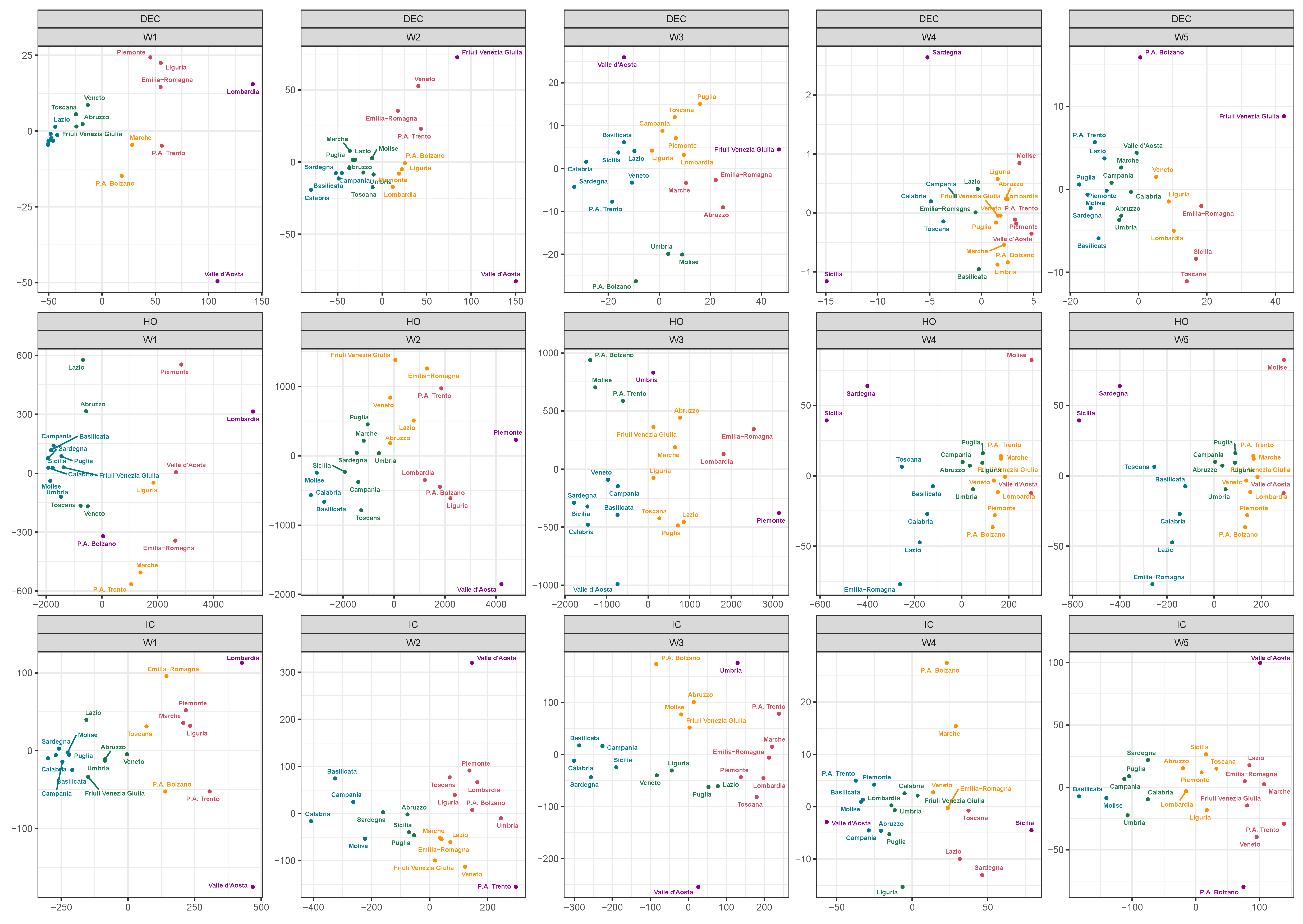
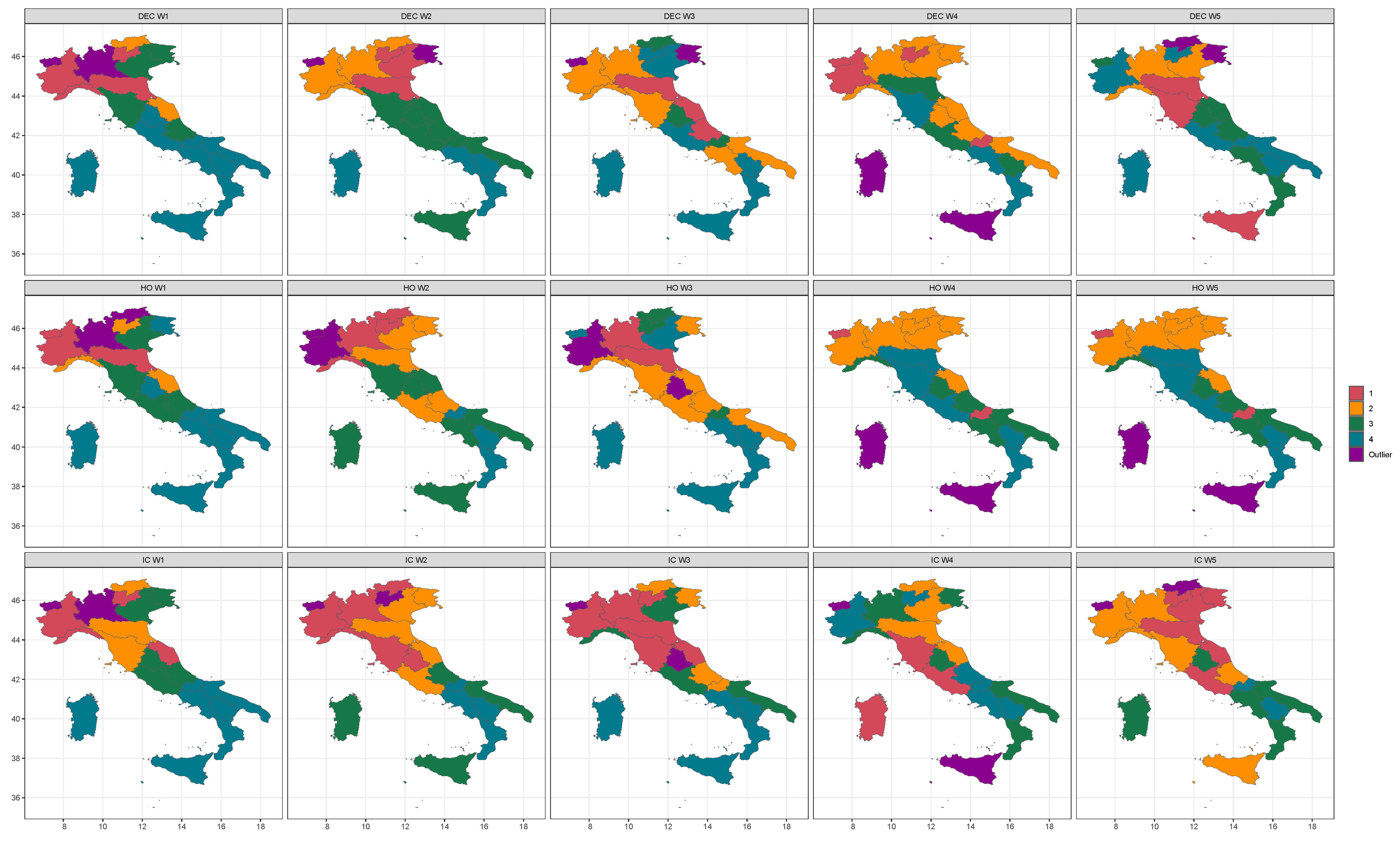
2. Time Series Clustering

Given a matrix $T\times n$, where T represents the days and n the number of regions, our methodological approach consists of three subsequent steps:

Step 1.

Compute a dissimilarity matrix D based on a given measure;

Step 2.

Apply a weighted multidimensional scaling (wMDS) procedure, storing the coordinates of the first two components;

Step 3.

Perform cluster analysis on the MDS reduced space to identify groups between the n regions.

In the following, we describe in detail each step with emphasis on the choice of a distance, the wMDS, and the clustering method.

2.1. Dissimilarities between Time Series

In the first step, a dissimilarity measure is computed for each pair of regional time series. The objective is to obtain a dissimilarity matrix D for estimating synthetic measures of the differences between geographical areas. There are different alternatives to compare time series, and some comprehensive overviews are in [14,17].

Epidemic-related time series are mainly driven by biological and physical mechanisms, usually modeled through differential equation models (see e.g., [18], for the COVID-19 case), taking into account factors such as the contagion spreading capability in terms of susceptible, immune, and recovered individuals. For such reasons, the use of model-based dissimilarities [19] and autocorrelation-based approaches (see e.g., [20]) appears not immediately suitable for COVID-19-related time series, especially because these dissimilarities rely on assumptions regarding, for instance, stationarity and/or ergodicity, which may be unreliable (for an exception, see [21]).

In view of the above, we rely on the following set of dissimilarity measures computed on pairs of time series $\mathbf{x},\mathbf{y}$ of the same length.

Euclidean

It is the most common distance, defined as:

$$d_E(\mathbf{x},\mathbf{y})=\sqrt{{(\mathbf{x}-\mathbf{y})}^{\top }(\mathbf{x}-\mathbf{y})}$$

(1)

Besides its wide applicability, its scale-invariance property [22] does not hold when data are not standardized, and it has the drawback of not considering the (possible) presence of correlation between series.

Pearson’s Correlation (Cor)

Two time series are considered similar if they share a linear trend, and the dissimilarity index is:

$$d_{Cor}(\mathbf{x},\mathbf{y})=1-{\displaystyle \frac{{(\mathbf{x}-\overline{x})}^{\top }(\mathbf{y}-\overline{y})}{\sqrt{{(\mathbf{x}-\overline{x})}^{\top }(\mathbf{x}-\overline{x})}\sqrt{{(\mathbf{y}-\overline{y})}^{\top }(\mathbf{y}-\overline{y})}}}$$

(2)

where $\overline{x},\overline{y}$ are the means of the two series. This measure may lead to misleading results in presence of spurious correlation or exogenous effects [23].

Dynamic Time Warping (DTW)

Introduced in [24], this method allows us to “warp” (compress and/or stretch) the series in time to detect a similarity that is not sensitive to (local) shifting and/or scaling effects. Let M be the set of all possible sequences of pairs $\mathbf{r}$ with length $m\le T$ preserving the observation order in the form:

$$\mathbf{r}=\left((x_{a_1},y_{b_1}),\dots ,(x_{a_m},y_{b_m})\right),$$

where the indices are set as $1=a_1\le \cdots \le a_i\le \cdots \le a_m=T$ and $1=b_1\le \cdots \le b_i\le \cdots \le b_m=T$. Then, the DTW distance [25] takes the following form:

$$d_{DTW}(\mathbf{x},\mathbf{y})=\underset{\mathbf{r}\in M}{min}\left(\sum _{h=1}^m|x_{a_h}-y_{b_h}|\right).$$

DTW is widely used for classification, clustering, and outlier detection purposes [26,27,28] and is suitable for time series with similar patterns but differences in shifting and/or scaling.

Complexity invariance dissimilarity (CID)

Complexity invariance dissimilarity [29] consists in applying a correction factor for an existing distance measures, i.e. the Euclidean, as follows:

$$d_{CID}(\mathbf{x},\mathbf{y})=d_E(\mathbf{x},\mathbf{y})·{\displaystyle \frac{max\left(CE\left(\mathbf{x}\right),CE\left(\mathbf{y}\right)\right)}{min\left(CE\left(\mathbf{x}\right),CE\left(\mathbf{y}\right)\right)}}$$

(3)

where the complexity correction factor $CE(·)$ is defined as

$$\begin{array}{ccc}\hfill CE\left(\mathbf{x}\right)=\sqrt{\sum _{t=2}^T{(x_t-x_{t-1})}^2},\hfill & \hfill & \hfill CE\left(\mathbf{y}\right)=\sqrt{\sum _{t=2}^T{(y_t-y_{t-1})}^2}.\hfill \end{array}$$

An advantage of this measure is that it does not rely on any specific serial features or on the specification of a (possibly underlying) model.

Fourier

A last option is the Fourier dissimilarity $d_F(\mathbf{x},\mathbf{y})$, which applies the n-point discrete Fourier transform of [30] on two time series, allowing the comparison of the similarity between two time sequences after converting them into a combination of structural elements, such as trend and/or cycle.

Important differences exist among the previously illustrated measures, since Euclidean and DTW evaluate the similarities by measuring the proximity on observations, while Pearson’s correlation detects differences in terms of temporal correlation and (linear) trend. On the other hand, Fourier dissimilarity is centered on a feature-based approach, consisting in judging the similarities between series over a set of chosen characteristics. Finally, CID belongs to the class of complexity-based dissimilarities, relying on the Kolmogorov complexity principle, as illustrated by [31].

2.2. Multidimensional Scaling

Multidimensional scaling, early introduced in the 1950s by [32] and recently reviewed in [33], is a dimensionality reduction technique. Given a dissimilarity matrix between a set of data, MDS finds a low-dimensional embedding of data points (coordinates) whose configuration minimizes a loss function [16]. Due to its flexibility, MDS has been introduced also in time series analysis (see e.g., [34]) and recently applied to different topics (see, e.g., [35,36,37], among others).

Starting from a $n\times n$ dissimilarity matrix D, classical MDS finds an $n\times m$ matrix $Z=({\mathbf{z}}_1,\dots ,{\mathbf{z}}_n)$, with $m\le n-1$, obtained by minimizing a cost function, called stress function [35,38], such that the reconstructed distance matrix is similar to the original dissimilarity matrix D. Classical MDS is based on ${\mathcal{L}}_2$ norm, i.e., the Euclidean distance.

Furthermore, since our aim is to take into account the degree of proximity between regions, we also employ a weighted multidimensional scaling technique (wMDS [39,40]). The ${\mathcal{L}}_2$ norm is multiplied by a set of point weights $\mathbf{\omega }=({\omega }_1,\dots ,{\omega }_n)$ such that high weights have a stronger influence on the result than low weights. To summarize, the stress function is defined as:

$$stres{s}_D({\mathbf{z}}_1,\dots ,{\mathbf{z}}_n)=\sqrt{\sum _{i<j}^n(d_{ij}-{\omega }_i\left|\right|{\mathbf{z}}_i-{\mathbf{z}}_j{\left|\right|)}^2}.$$

(4)

Setting equal weights, i.e., ${\omega }_i=1$, for each $i=1,\dots ,n$, returns to ordinary MDS. To assess the adequacy of the final model, some goodness-of-fit can be used following the suggestions of [38].

Similarly to principal component analysis, the reduced space generated by MDS can be used as starting point for subsequent analyses. Then, a clustering algorithm can be performed on the coordinates (of the reduced space) of MDS [41].

2.3. Clustering

Different procedures (such as hierarchical and point-based algorithms) should be suitable to perform a cluster analysis on the wMDS coordinates map. For an overview of modern clustering techniques in time series, see, e.g., [42].

Moreover, in our case, both the geographical spread of the pandemic and population density can determine remarkable differences in terms of hospitalization rates [43]. To mitigate this risk of regional outliers in the data, generating potential spurious clusters, the use of a robust algorithm is strongly suggested. For this reason, we employ the trimmed k-means algorithm, proposed by [44] and developed by [45]. This algorithm applies k-means clustering on a subset of initial data defined by a trimming level $\alpha$ and by a penalty function that isolates extreme values [46].

A relevant topic in cluster analysis is related to the choice of the k number of groups. Our strategy is purely data-driven and it is based on the minimization of the within-cluster variance and the use of the elbow criterion.

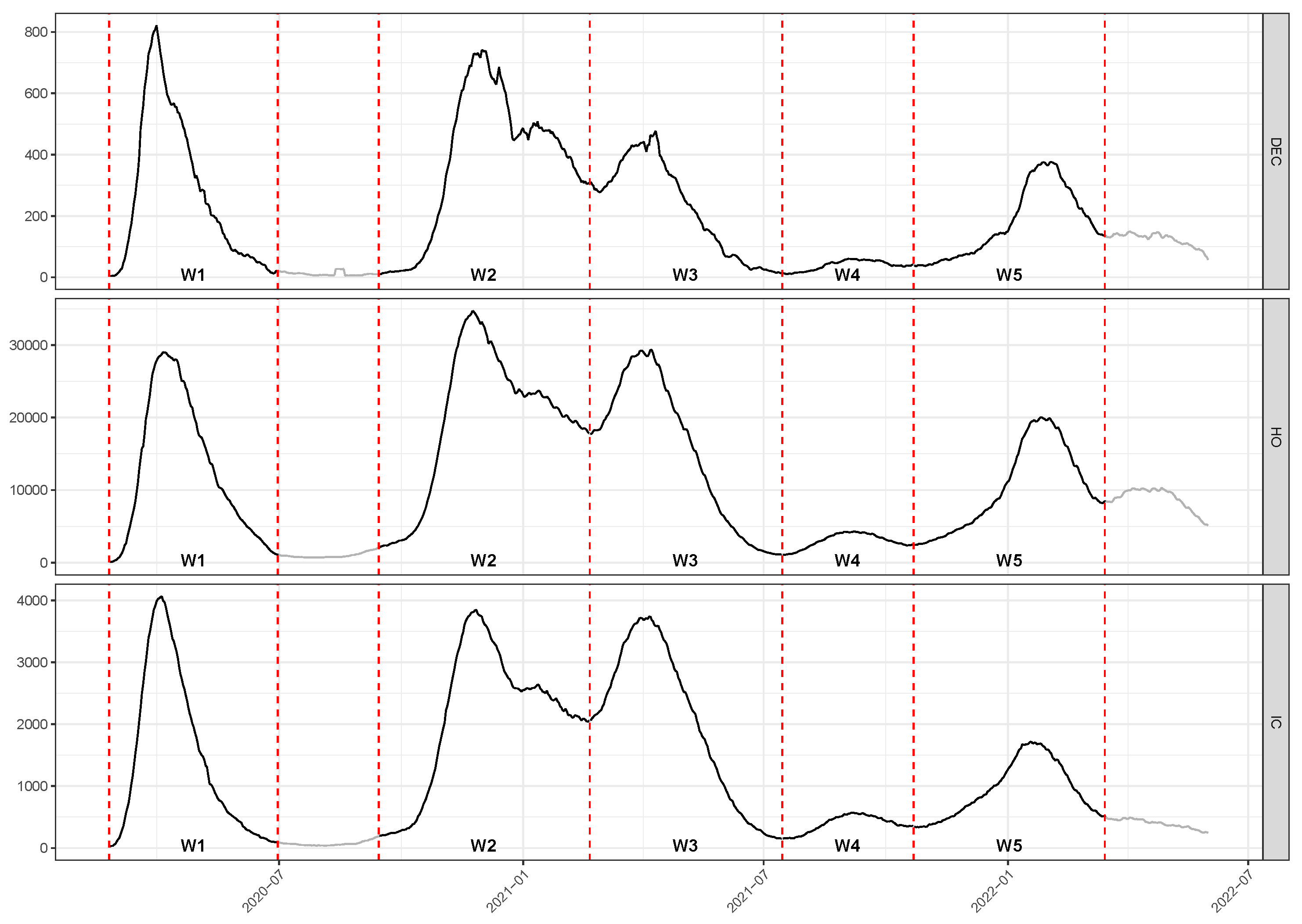
3. Data and Descriptive Statistics

Data adopted in this work consist of daily regional time series reporting (a) the number of deceased patients, (b) the number of patients treated in IC units, and (c) the number of patients admitted in the other hospital wards are retrieved through the official website of Italian Civil Protection (https://github.com/pcm-dpc/COVID-19, accessed on 10 January 2023). All patients were positive for the COVID-19 test (nasal and oropharyngeal swab). To take into account the different sizes in terms of inhabitants (a), (b), and (c) are normalized according to the population of each territorial unit (estimated on 1 January 2020). The rates of patients deceased (DEC), treated in intensive care units (IC), and hospitalized (HO) in other hospital wards are then multiplied by 100,000. In addition, the series of deceased patients is also smoothed using a moving average 7-day rolling window.

According to the literature, history records, and graphical inspection, the whole dataset contains five identified waves of COVID-19

Wave 1 (W1):

$T_1=128$ days from 24 February to 30 June 2020

Wave 2 (W2):

$T_2=159$ days from 14 September 2020 to 19 February 2021

Wave 3 (W3):

$T_3=145$ days from 20 February to 14 July 2021

Wave 4 (W4):

$T_4=99$ days from 15 July to 21 October 2020

Wave 5 (W5):

$T_5=145$ days from 22 October to 15 March 2022

These waves are summarized through Figure 1 for the three considered time series at the national level. The date/trend may also depend on external factors, such as the implementation of restrictive measures introduced by the Italian Government (see e.g., [47,48]), which influenced the observed differences between W1 and W2. We have to remark that a full national lockdown was held between 9 March and 18 May 2020. Then, starting from September 2020, four progressive levels of restriction [49] were introduced according to the regional healthcare situation (number of cases, beds in ICU, beds in other hospital wards). In 2021, for a large part of winter and spring, all Italian regions were in the “worst” level of restriction (similar to the national lockdown), while the COVID vaccines were introduced in January 2021. The tougher restrictions have been phased out starting from the end of April 2021.

Descriptive analysis is depicted in

Table 1. Descriptive statistics of DEC in W1–W5.

	W1			W2			W3			W4			W5
DEC	Peak	s.d.	MAD	Peak	s.d.	MAD	Peak	s.d.	MAD	Peak	s.d.	MAD	Peak	s.d.	MAD
Abruzzo	0.85	0.24	0.31	1.42	0.35	0.40	1.35	0.42	0.46	0.10	0.03	0.03	0.65	0.18	0.19
Basilicata	0.23	0.06	0.00	1.14	0.26	0.28	0.89	0.23	0.23	0.15	0.04	0.04	0.71	0.21	0.21
Calabria	0.23	0.06	0.01	0.51	0.13	0.13	0.44	0.11	0.13	0.18	0.05	0.06	0.63	0.16	0.25
Campania	0.22	0.07	0.04	0.90	0.27	0.30	0.80	0.22	0.29	0.15	0.03	0.04	0.62	0.15	0.12
Emilia-Romagna	2.11	0.70	0.57	1.64	0.55	0.57	1.20	0.40	0.49	0.13	0.03	0.03	0.90	0.25	0.26
Friuli Venezia Giulia	0.71	0.21	0.16	2.74	0.90	1.05	1.69	0.56	0.59	0.15	0.03	0.03	1.07	0.25	0.31
Lazio	0.31	0.07	0.07	0.89	0.28	0.23	0.65	0.20	0.28	0.10	0.02	0.03	0.47	0.11	0.12
Liguria	2.02	0.66	0.70	1.78	0.47	0.51	1.02	0.26	0.26	0.10	0.02	0.01	0.80	0.23	0.31
Lombardia	4.43	1.28	0.95	2.01	0.54	0.58	0.96	0.33	0.42	0.06	0.01	0.02	0.90	0.26	0.26
Marche	2.07	0.63	0.33	0.90	0.32	0.29	0.92	0.34	0.37	0.09	0.03	0.03	0.60	0.14	0.18
Molise	0.33	0.08	0.00	1.31	0.41	0.45	1.31	0.39	0.38	0.14	0.03	0.00	0.65	0.18	0.14
P.A. Bolzano	2.64	0.63	0.04	2.23	0.59	0.56	1.51	0.36	0.16	0.11	0.03	0.04	0.54	0.13	0.12
P.A. Trento	2.85	0.86	0.27	2.14	0.69	0.94	0.63	0.19	0.20	0.11	0.03	0.04	0.53	0.13	0.16
Piemonte	2.10	0.65	0.67	1.94	0.58	0.74	0.98	0.31	0.43	0.06	0.02	0.02	0.64	0.17	0.18
Puglia	0.37	0.10	0.07	1.01	0.31	0.28	1.05	0.32	0.35	0.10	0.02	0.03	0.48	0.14	0.12
Sardegna	0.28	0.08	0.03	0.84	0.22	0.23	0.45	0.12	0.12	0.26	0.06	0.06	0.49	0.16	0.12
Sicilia	0.18	0.05	0.02	0.94	0.28	0.27	1.01	0.20	0.14	0.41	0.11	0.14	0.91	0.27	0.29
Toscana	0.68	0.21	0.19	1.52	0.43	0.48	0.83	0.25	0.31	0.18	0.04	0.03	0.84	0.28	0.20
Umbria	0.29	0.09	0.05	1.31	0.41	0.48	1.31	0.34	0.26	0.11	0.04	0.05	0.65	0.19	0.18
Valle d’Aosta	5.46	1.43	0.34	5.23	1.45	1.01	1.71	0.38	0.17	0.11	0.03	0.00	0.91	0.22	0.17
Veneto	0.76	0.26	0.29	2.11	0.71	1.11	0.73	0.22	0.31	0.08	0.02	0.02	0.65	0.20	0.27

,

Table 2. Descriptive statistics of IC in W1–W5.

	W1			W2			W3			W4			W5
IC	Peak	s.d.	MAD	Peak	s.d.	MAD	Peak	s.d.	MAD	Peak	s.d.	MAD	Peak	s.d.	MAD
Abruzzo	5.79	1.83	0.90	5.87	1.70	1.98	7.17	2.53	3.45	1.07	0.27	0.23	3.13	0.81	0.68
Basilicata	3.38	1.07	0.26	5.33	1.41	1.05	3.02	0.98	1.05	0.71	0.25	0.26	1.24	0.32	0.26
Calabria	1.18	0.34	0.15	2.72	0.65	0.46	2.57	0.71	0.84	0.92	0.23	0.30	1.95	0.47	0.57
Campania	3.12	0.73	0.41	3.91	0.89	0.79	3.17	0.94	0.91	0.53	0.08	0.10	1.76	0.48	0.33
Emilia-Romagna	8.41	2.79	3.39	5.79	1.92	1.13	9.01	2.91	4.27	1.23	0.31	0.20	3.45	0.93	1.25
Friuli Venezia Giulia	5.02	1.54	0.37	5.68	1.88	0.98	7.08	2.58	3.72	1.23	0.34	0.37	3.62	0.86	0.98
Lazio	3.45	1.11	1.01	6.19	1.88	1.24	6.77	1.98	2.52	1.22	0.21	0.20	3.52	0.90	1.08
Liguria	11.54	3.80	3.16	7.93	1.90	1.48	5.61	1.62	1.58	0.97	0.19	0.19	3.10	0.76	1.05
Lombardia	13.73	4.51	4.24	9.43	2.81	3.07	8.65	2.83	4.09	0.63	0.12	0.15	2.74	0.75	1.02
Marche	11.08	3.70	3.11	6.16	2.05	1.41	10.29	3.31	4.76	1.77	0.49	0.73	4.26	1.00	1.17
Molise	2.94	0.81	0.97	4.58	1.27	0.97	8.51	2.44	3.64	0.65	0.22	0.24	1.96	0.39	0.49
P.A. Bolzano	12.24	3.66	1.40	8.28	2.60	2.79	7.53	2.43	1.12	1.88	0.58	0.84	4.14	1.19	1.95
P.A. Trento	14.97	4.84	2.19	9.79	3.55	3.84	10.16	3.43	4.66	0.92	0.26	0.27	5.17	1.64	2.47
Piemonte	10.40	3.44	3.06	9.27	2.81	2.99	8.68	2.78	3.86	0.57	0.18	0.24	3.56	1.03	0.87
Puglia	3.95	0.88	0.70	5.63	1.71	1.21	7.10	2.34	3.11	0.77	0.13	0.11	1.74	0.47	0.37
Sardegna	1.89	0.60	0.81	4.64	0.99	1.18	3.72	1.09	1.36	1.83	0.41	0.50	2.07	0.58	0.86
Sicilia	1.60	0.49	0.36	5.06	1.52	1.11	3.78	1.10	1.29	2.40	0.64	0.83	3.40	0.87	0.74
Toscana	7.96	2.61	2.39	7.99	2.28	2.52	7.67	2.46	3.08	1.58	0.39	0.54	3.70	0.87	0.83
Umbria	5.44	1.84	0.67	9.64	2.75	2.86	9.75	3.33	3.87	0.91	0.25	0.34	1.59	0.24	0.25
Valle d’Aosta	21.49	6.68	1.18	13.53	4.01	2.36	11.94	3.74	2.36	0.80	0.11	0.00	6.37	1.82	1.18
Veneto	7.26	2.39	1.18	7.58	2.64	3.66	6.22	1.90	2.39	1.16	0.31	0.35	4.20	1.19	1.63

and

Table 3. Descriptive statistics of HO in W1–W5.

	W1			W2			W3			W4			W5
HO	Peak	s.d.	MAD	Peak	s.d.	MAD	Peak	s.d.	MAD	Peak	s.d.	MAD	Peak	s.d.	MAD
Abruzzo	27.52	9.33	14.24	54.44	15.67	13.23	52.23	18.90	29.16	6.79	1.53	1.75	40.79	11.97	12.66
Basilicata	11.55	4.16	3.42	29.31	7.61	6.32	31.98	10.17	15.54	9.95	2.23	3.03	20.43	6.05	8.30
Calabria	9.40	2.92	2.89	22.34	6.50	6.78	24.75	7.33	9.59	9.30	2.25	3.08	22.91	6.12	8.79
Campania	10.72	3.71	5.60	40.18	9.66	7.27	27.92	9.10	6.31	6.53	1.23	1.85	24.20	7.24	6.77
Emilia-Romagna	88.44	30.55	23.47	65.34	22.44	18.27	83.01	27.33	40.56	10.09	2.05	1.60	60.57	17.42	21.58
Friuli Venezia Giulia	19.42	5.71	7.56	57.85	21.50	18.48	55.96	18.99	24.34	4.36	1.17	1.16	42.71	10.21	11.16
Lazio	24.97	8.77	11.70	57.97	15.87	12.24	55.54	17.07	22.58	9.15	1.86	1.55	36.50	9.79	11.31
Liguria	74.36	25.06	24.95	90.41	22.80	16.06	44.56	15.70	16.64	6.00	1.40	1.82	49.21	15.42	21.46
Lombardia	120.04	38.94	42.15	83.40	23.88	22.40	71.35	24.15	35.60	4.35	0.87	0.76	36.97	10.42	9.84
Marche	65.63	24.45	19.25	39.21	13.84	6.71	53.24	18.94	29.65	4.52	1.08	1.17	22.75	6.30	9.43
Molise	11.45	3.62	3.88	26.18	7.83	4.85	35.67	11.66	11.89	4.25	1.20	0.97	14.72	4.00	4.37
P.A. Bolzano	61.18	16.90	13.12	91.68	26.38	20.93	48.76	13.29	12.42	6.02	1.42	1.54	26.17	4.01	3.77
P.A. Trento	66.53	24.13	14.25	80.58	28.26	43.98	40.10	14.50	16.71	5.54	1.26	0.96	29.20	8.46	10.00
Piemonte	81.56	27.56	38.12	119.94	36.15	42.06	89.27	30.11	45.98	4.77	1.16	1.11	49.12	15.70	17.78
Puglia	16.08	5.53	6.51	42.02	13.03	6.00	50.36	16.61	20.50	6.23	1.29	1.60	18.69	6.28	5.57
Sardegna	7.68	2.63	4.16	37.88	10.09	8.95	23.05	6.59	8.18	14.64	3.96	5.29	25.19	8.07	9.31
Sicilia	11.36	4.13	3.02	32.08	8.90	8.05	25.48	7.17	9.16	17.10	4.55	6.11	29.92	8.91	13.55
Toscana	30.81	10.74	6.96	49.12	13.82	14.33	46.22	15.40	20.87	11.37	2.86	3.16	36.84	11.28	14.89
Umbria	19.95	6.35	3.87	53.40	14.49	12.61	53.85	17.83	22.44	6.12	1.67	1.51	25.40	8.03	12.86
Valle d’Aosta	104.24	31.94	30.67	135.28	41.62	46.60	54.11	16.22	12.98	3.98	1.14	1.18	64.46	17.02	17.70
Veneto	35.02	12.13	9.49	55.26	19.69	28.62	35.06	11.26	16.49	4.65	1.05	0.92	32.29	9.61	11.68

containing the maximum, the standard deviation, and the median absolute deviation (MAD) of the series (maxima are highlighted in bold). The anomaly of the small Italian region (Valle D’Aosta) emerges in W1, W2, and W3 for what concerns DEC and IC, while Lombardia, which is the largest and most populous region, dominates other territories, especially when considering HO of W1. Regarding the deceased (DEC), the northeastern region of Friuli-Venezia Giulia presents the highest variability in W3 and W5, while the island region of Sicily presents the maximum and the largest variability in W4. This region confirmed its critical situation in W4 also looking at the IC and the HO series. The northwestern region of Piemonte also shows the highest value of HO in W3.

4. Grouping Regions by Clustering and Discussion

In order to confirm and deepen the descriptive results of Section 3, we perform a cluster analysis following the scheme proposed in Section 2. We compute wMDS according to the five different dissimilarities, using a set of weights $\omega$. Several possibilities for the choice of such weights can be explored. To pursue our aim, we take into account some spatial features of the regions, and here we selected the weights proportional to the number of bordering neighborhoods for each region, ensuring to add some spatial features to the analysis. The optimal number of clusters, selected looking at the within-cluster variance using the elbow criterion, is equal to four, excluding the outlying values.

Table 4. Goodness-of-fit measures ($R^2$ and GoF in semi-rows) for the considered series.

	DEC						HO						IC
	W1	W2	W3	W4	W5		W1	W2	W3	W4	W5		W1	W2	W3	W4	W5
CID	0.5262	0.6510	0.7988	0.7192	0.8241		0.5997	0.6823	0.7537	0.7196	0.7196		0.5211	0.8079	0.8167	0.7649	0.7638
	0.9969	0.9830	0.8320	0.9411	0.7782		0.9953	0.9671	0.9106	0.9326	0.9326		0.9965	0.9193	0.8648	0.9142	0.9381
Cor	0.8441	0.8237	0.8342	0.5388	0.7939		0.9520	0.9603	0.9811	0.9239	0.9239		0.9110	0.9252	0.9416	0.7199	0.8292
	0.5825	0.6851	0.6746	0.3491	0.5647		0.8236	0.8424	0.9092	0.6525	0.6525		0.7328	0.7878	0.8113	0.5690	0.6995
DTW	0.9525	0.8975	0.8149	0.9419	0.8085		0.9430	0.9128	0.9024	0.9436	0.9436		0.9264	0.9227	0.8955	0.8916	0.8951
	0.9852	0.8976	0.7863	0.8332	0.7131		0.9922	0.9016	0.9404	0.9535	0.9535		0.9757	0.8531	0.8635	0.8318	0.9180
Euclidean	0.9958	0.9894	0.9507	0.9856	0.9249		0.9985	0.9877	0.9917	0.9951	0.9951		0.9951	0.9552	0.9800	0.9807	0.9791
	0.9408	0.8642	0.7608	0.7689	0.7176		0.9807	0.9116	0.9544	0.9340	0.9340		0.9542	0.8343	0.8961	0.8601	0.8902
Fourier	0.9975	0.9930	0.9663	0.9924	0.9611		0.9992	0.9933	0.9951	0.9979	0.9979		0.9970	0.9760	0.9878	0.9904	0.9872
	0.9584	0.8974	0.7918	0.8533	0.7931		0.9876	0.9394	0.9668	0.9631	0.9631		0.9682	0.8818	0.9234	0.9127	0.9264

reports two measures of goodness of fit: $R^2$ type and GoF, i.e., the ratio of the cumulative eigenvalues. These measures are useful to compare the performance of wMDS according to the different dissimilarities. They produce almost the same performance ranking: Fourier appears to be the best dissimilarity, shortly followed by Euclidean and DTW. The CID shares the worst performances for DEC, HO, and IC in all considered waves, followed by the Cor distance which presents low values of performance indicators for DEC. A possible explanation is the sensitivity to outliers [29] of CID.

Figure 2 displays the main results of wMDS, distinguishing between four levels of critical issues experienced by the RHS for the results based on the Fourier dissimilarity. The other achievements, here not presented for sake of brevity, are very similar. Outlying performances are colored in Violet. A first cluster (in Red) includes “critical” regions, while a group depicted in Yellow contains territories with high pressure in their RHS. Regions involved in the Green cluster experimented with moderate pressure on RHS, while the color Blue indicates territories suffering from low pressure. These clusters may also be interpreted as a ranking of the health service risk. Figure 3 shows the same information as Figure 2 from a geographical perspective. These choropleth maps are useful to highlight spatial and temporal changes in the performance of RHS among the waves.

First Wave

As regards the DEC during W1, leaving apart the two outliers (Lombardia and Valle d’Aosta), the “red” cluster is composed of four northern regions (Piemonte, Liguria, P.A. of Trento, Emilia-Romagna). The group of high pressure is composed of only two regions (P.A. of Bolzano and Marche), while the green cluster involves Veneto, Friuli-Venezia Giulia (located in the northeast) and Toscana and Abruzzo (located in the center and south of Italy, respectively). The last group includes nine regions, five of which are located in southern Italy and the two Islands. These groups are practically the same for the IC rates except for Marche, involved in the critical cluster.

The situation is also quite similar concerning HO: outliers are Lombardia and P.A. of Bolzano; the “critical” cluster is composed of Valle D’Aosta, Piemonte, and Emilia-Romagna, while the “yellow” group contains Liguria (northwest), P.A. of Trento (northeast) and Marche (central Italy). Two regions with moderate pressure are located in the center (Toscana and Lazio), while this cluster also includes Veneto (northeast) and Abruzzo (south). Other southern regions and the two islands, accompanied by Umbria (central Italy) and Friuli-Venezia Giulia (northeast), are classified in the group presenting low pressure in terms of RHS.

Second Wave

In W2, the clustering procedure identifies Valle D’Aosta as an outlier for the three considered series, confirming the results of the descriptive analysis. Regarding HO, even the neighboring region of Piemonte is classified as an outlier.

Concerning rates for the deceased, regions classified in the critical and high-pressure clusters are all located in northern Italy. Regions of central Italy, three regions of southern Italy, and Sicily (island) are classified in the group of moderate pressure. The “blue” group includes three regions of the south (Campania, Basilicata, and Calabria) and the island of Sardegna. In terms of HO, two neighboring regions of Lazio (central) and Abruzzo (south) belong to the high-pressure group, while the critical group includes Lombardia, Liguria, P.A. of Trento, and P.A. of Bolzano (all located in northern Italy). Regarding IC rates, the groups of critical and high pressure are composed of six (Piemonte, Lombardia, P.A. of Bolzano, Liguria, Toscana, and Umbria) and five Regions (Friuli-Venezia Giulia, Piemonte, Emilia-Romagna, Marche, Lazio), respectively, even excluding any region of southern Italy and the two islands.

Third Wave

In the third wave, Valle d’Aosta remains a “negative” outlier considering DEC and IC. Surprisingly, it belongs to the low-pressure group for HO, along with Veneto, three southern regions (Campania, Basilicata, Sicilia), and the two islands. The small region of Umbria (located in the center of Italy) represents a “positive” outlier both for the IC and the HO due to its decreasing trends in the considered window. In this wave, some regions of the south belong to the high-pressure group: Campania and Puglia for DEC, Puglia, and Abruzzo for HO, along with Abruzzo and Molise for IC. The “red” group contains only two regions for HO (the neighboring Lombardia and Emilia-Romagna), three regions for DEC (Emilia-Romagna, Marche, and Abruzzo), and six regions for IC (Piemonte, Lombardia, P.A. of Trento, Emilia-Romagna, Toscana, and Marche).

Fourth and Fifth Waves

As mentioned, in the fourth wave, the levels of the considered series are the lowest among the five waves, even due to the spread of vaccines throughout the overall Italian regions. Nonetheless, the islands (Sicilia and Sardegna) share the highest pressure, compared to the other regions, for DEC, HO, and IC. In particular, Sicilia and Sardegna are together classified as outliers for DEC and HO. Critical pressure of HO is observed for the two smallest regions (Valle D’Aosta and Molise), while the yellow group (“high pressure”) contains all the northern regions except Liguria (belonging to the moderate pressure cluster) and Emilia-Romagna. This situation is exactly reproduced in W5. Considering IC occupation, the “red” group is composed of two neighboring regions of the center (Toscana and Lazio) and the island of Sardegna. It is remarkable that, after three waves, Lombardia belongs to the moderate pressure cluster for the first time. If the geography of the disease appears fundamental in W1 and W2, especially regarding adjoining territories of Lombardia, from W3 this effect is less evident. Thus, regions improving (e.g., Emilia-Romagna in W4 and W5 considering HO) or worsening (such as Lazio in W4 and W5 for the IC rates), their clustering “ranking” can be easily observed. As mentioned, the differences in restrictive measures imposed by the government in the overall period may have a role in these results.

5. Concluding Remarks

The COVID-19 pandemic has put a strain on the Italian healthcare system. The reactions of RHS play a relevant role to mitigate the health crisis at the territorial level and to guarantee equitable access to healthcare.

This work helps to understand similarities and divergences between the Italian regions in relation to the health pressure considering the five waves of the virus. Crucial measures such as DEC, HO, and IC rates, can help to make a comparison between the five waves allowing us to understand differences in the reactions to pandemic shocks of RHS. Although Northern Italy represented the epicenter of the COVID-19 spread in the W1, some regions seem to have succeeded in avoiding hospitals overcrowding (see e.g., Veneto and Friuli-Venezia Giulia), while the southern regions (and islands) definitively suffered from less pressure. Furthermore, starting from W2, the difference appears slightly smoothed and the cluster sizes seem more homogeneous. The detection of clusters represents a starting point for the improvement of health governance and can be used to monitor potential imbalances in future epidemic diseases.

We pointed out that the performance results of Section 4 can be affected by the combination of different components such as (a) the main features of the regional series, (b) the used dissimilarity metrics, (c) the selected method of dimensionality reduction, and (d) the choice of weights. In addition, the clustering results may depend on the selection of some parameters such as the number of clusters and the trimming parameter.

Further analysis may employ other dedicated indicators coming, for instance, from the Italian National Institute of Statistics (see, for example, the BES indicators of the domain “Health” and “Quality of services” https://www.istat.it/it/files//2021/03/BES_2020.pdf accessed on 10 January 2023) or using different proposals for combining wMDS with dissimilarity measures and clustering (see, e.g., [50]). For example, the rate of doctors and nurses and the presence of public (or private) hospitals are indicators that may be included in the analysis. Considering other clustering approaches, a simulation study will be carried out to compare the performance of different methods after generating various scenarios of the propagation of an epidemic. Following a different methodological approach, the recent method proposed in [51] should be applied to those types of data to include more complex spatial relationships between territories.

References

- Capolongo, S.; Gola, M.; Brambilla, A.; Morganti, A.; Mosca, E.I.; Barach, P. Covid-19 and Healthcare facilities: A decalogue of design strategies for resilient hospitals. Acta Bio Med. 2020, 91, 50–60. [Google Scholar]
- Pecoraro, F.; Luzi, D.; Clemente, F. Analysis of the different approaches adopted in the Italian regions to care for patients affected by Covid-19. Int. J. Environ. Res. Public Health 2021, 18, 848. [Google Scholar] [PubMed]
- Han, E.; Tan, M.M.J.; Turk, E.; Sridhar, D.; Leung, G.M.; Shibuya, K.; Asgari, N.; Oh, J.; García-Basteiro, A.L.; Hanefeld, J.; et al. Lessons learnt from easing Covid-19 restrictions: An analysis of countries and regions in Asia Pacific and Europe. Lancet 2020, 396, 1525–1534. [Google Scholar] [CrossRef] [PubMed]
- Ascani, A.; Faggian, A.; Montresor, S. The geography of Covid-19 and the structure of local economies: The case of Italy. J. Reg. Sci. 2020, 61, 2. [Google Scholar] [CrossRef]
- Beria, P.; Lunkar, V. Presence and mobility of the population during the first wave of Covid-19 outbreak and lockdown in Italy. Sustain. Cities Soc. 2021, 65, 102616. [Google Scholar]
- Marziano, V.; Guzzetta, G.; Rondinone, B.M.; Boccuni, F.; Riccardo, F.; Bella, A.; Poletti, P.; Trentini, F.; Pezzotti, P.; Brusaferro, S.; et al. Retrospective analysis of the Italian exit strategy from Covid-19 lockdown. Proc. Natl. Acad. Sci. USA 2021, 118, e2019617118. [Google Scholar] [CrossRef]
- Bontempi, E. The Europe second wave of Covid-19 infection and the Italy “strange” situation. Environ. Res. 2021, 193, 110476. [Google Scholar] [CrossRef]
- Boriani, G.; Guerra, F.; De Ponti, R.; D’Onofrio, A.; Accogli, M.; Bertini, M.; Bisignani, G.; Forleo, G.B.; Landolina, M.; Lavalle, C.; et al. Five waves of COVID-19 pandemic in Italy: Results of a national survey evaluating the impact on activities related to arrhythmias, pacing, and electrophysiology promoted by AIAC (Italian Association of Arrhythmology and Cardiac Pacing). Intern. Emerg. Med. 2022, 18, 137–149. [Google Scholar] [CrossRef]
- Pecoraro, F.; Clemente, F.; Luzi, D. The efficiency in the ordinary hospital bed management in Italy: An in-depth analysis of intensive care unit in the areas affected by Covid-19 before the outbreak. PLoS ONE 2020, 15, e0239249. [Google Scholar] [CrossRef]
- Agosto, A.; Giudici, P. A Poisson autoregressive model to understand Covid-19 contagion dynamics. Risks 2020, 8, 77. [Google Scholar] [CrossRef]
- Farcomeni, A.; Maruotti, A.; Divino, F.; Lasinio, G.J.; Lovison, G. An ensemble approach to short-term forecast of Covid-19 intensive care occupancy in Italian Regions. arXiv 2020, arXiv:2005.11975. [Google Scholar] [CrossRef] [PubMed]
- James, N.; Menzies, M. Cluster-based dual evolution for multivariate time series: Analyzing Covid-19. Chaos Interdiscip. J. Nonlinear Sci. 2020, 30, 061108. [Google Scholar] [CrossRef] [PubMed]
- Rojas, I.; Rojas, F.; Valenzuela, O. Estimation of Covid-19 dynamics in the different states of the United States using Time-Series Clustering. medRxiv 2020. [Google Scholar] [CrossRef]
- Studer, M.; Ritschard, G. What matters in differences between life trajectories: A comparative review of sequence dissimilarity measures. J. R. Stat. Soc. Ser. A (Stat. Soc.) 2016, 179, 481–511. [Google Scholar] [CrossRef] [Green Version]
- Kruskal, J.B. Multidimensional Scaling; Sage: Newcastle upon Tyne, UK, 1978; Number 11. [Google Scholar]
- Mead, A. Review of the development of multidimensional scaling methods. J. R. Stat. Soc. Ser. D (Stat.) 1992, 41, 27–39. [Google Scholar] [CrossRef]
- Górecki, T.; Piasecki, P. A Comprehensive Comparison of Distance Measures for Time Series Classification. In Proceedings of the Workshop on Stochastic Models, Statistics and their Application, Dresden, Germany, 6–8 March 2019; Springer International Publishing: Berlin/Heidelberg, Germany, 2019; pp. 409–428. [Google Scholar]
- Cooper, I.; Mondal, A.; Antonopoulos, C.G. A SIR model assumption for the spread of COVID-19 in different communities. Chaos Solitons Fractals 2020, 139, 110057. [Google Scholar] [CrossRef]
- Piccolo, D. A distance measure for classifying ARIMA models. J. Time Ser. Anal. 1990, 11, 153–164. [Google Scholar] [CrossRef]
- D’Urso, P.; Maharaj, E.A. Autocorrelation-based fuzzy clustering of time series. Fuzzy Sets Syst. 2009, 160, 3565–3589. [Google Scholar] [CrossRef]
- Fenga, L. CoViD–19: An Automatic, Semiparametric Estimation Method for the Population Infected in Italy. PeerJ 2021, 9, e10819. [Google Scholar] [CrossRef]
- Iglesias, F.; Kastner, W. Analysis of similarity measures in times series clustering for the discovery of building energy patterns. Energies 2013, 6, 579–597. [Google Scholar] [CrossRef] [Green Version]
- Lee Rodgers, J.; Nicewander, W.A. Thirteen ways to look at the correlation coefficient. Am. Stat. 1988, 42, 59–66. [Google Scholar] [CrossRef]
- Berndt, D.J.; Clifford, J. Using dynamic time warping to find patterns in time series. In Proceedings of the KDD Workshop, Seattle, WA, USA, 31 July–1 August 1994; Volume 10, pp. 359–370. [Google Scholar]
- Giorgino, T. Computing and visualizing dynamic time warping alignments in R: The dtw package. J. Stat. Softw. 2009, 31, 1–24. [Google Scholar] [CrossRef] [Green Version]
- Montero, P.; Vilar, J.A. TSclust: An R Package for Time Series Clustering. J. Stat. Softw. 2014, 62, 1–43. [Google Scholar] [CrossRef] [Green Version]
- Tormene, P.; Giorgino, T.; Quaglini, S.; Stefanelli, M. Matching incomplete time series with dynamic time warping: An algorithm and an application to post-stroke rehabilitation. Artif. Intell. Med. 2009, 45, 11–34. [Google Scholar] [CrossRef]
- Benkabou, S.E.; Benabdeslem, K.; Canitia, B. Unsupervised outlier detection for time series by entropy and dynamic time warping. Knowl. Inf. Syst. 2018, 54, 463–486. [Google Scholar] [CrossRef]
- Batista, G.E.; Wang, X.; Keogh, E.J. A complexity-invariant distance measure for time series. In Proceedings of the 2011 SIAM International Conference on Data Mining, SIAM, 2011, Mesa, AZ, USA, 28–30 April 2011; pp. 699–710. [Google Scholar]
- Agrawal, R.; Faloutsos, C.; Swami, A. Efficient similarity search in sequence databases. In Proceedings of the International Conference on Foundations of Data Organization and Algorithms, Chicago, IL, USA, 13–15 October 1993; Springer: Berlin/Heidelberg, Germany, 1993; pp. 69–84. [Google Scholar]
- Li, M.; Vitányi, P. An Introduction to Kolmogorov Complexity and Its Applications; Springer: Berlin/Heidelberg, Germany, 2008; Volume 3. [Google Scholar]
- Torgerson, W.S. Multidimensional scaling: I. Theory and method. Psychometrika 1952, 17, 401–419. [Google Scholar] [CrossRef]
- Saeed, N.; Nam, H.; Haq, M.I.U.; Muhammad Saqib, D.B. A survey on multidimensional scaling. ACM Comput. Surv. (CSUR) 2018, 51, 1–25. [Google Scholar] [CrossRef] [Green Version]
- Piccolo, D. Una rappresentazione multidimensionale per modelli statistici dinamici. Atti Della XXXII Riun. Sci. Della SIS 1984, 2, 149–160. [Google Scholar]
- Tenreiro Machado, J.; Lopes, A.M.; Galhano, A.M. Multidimensional scaling visualization using parametric similarity indices. Entropy 2015, 17, 1775–1794. [Google Scholar] [CrossRef] [Green Version]
- Di Iorio, F.; Triacca, U. Distance Between VARMA Models and Its Application to Spatial Differences Analysis in the Relationship GDP-Unemployment Growth Rate in Europe. In Proceedings of the International Work-Conference on Time Series Analysis, Granada, Spain, 1–20 September 2017; Springer: Berlin/Heidelberg, Germany, 2017; pp. 203–215. [Google Scholar]
- He, J.; Shang, P.; Xiong, H. Multidimensional scaling analysis of financial time series based on modified cross-sample entropy methods. Phys. A Stat. Mech. Its Appl. 2018, 500, 210–221. [Google Scholar]
- Mardia, K.V. Some properties of clasical multi-dimesional scaling. Commun. Stat.-Theory Methods 1978, 7, 1233–1241. [Google Scholar] [CrossRef]
- Kent, J.; Bibby, J.; Mardia, K. Multivariate Analysis; Academic Press: Amsterdam, The Netherlands, 1979; Chapter 14. [Google Scholar]
- Greenacre, M. Weighted metric multidimensional scaling. In New Developments in Classification and Data Analysis; Springer: Berlin/Heidelberg, Germany, 2005; pp. 141–149. [Google Scholar]
- Kruskal, J. The relationship between multidimensional scaling and clustering. In Classification and Clustering; Elsevier: Amsterdam, The Netherlands, 1977; pp. 17–44. [Google Scholar]
- Saxena, A.; Prasad, M.; Gupta, A.; Bharill, N.; Patel, O.P.; Tiwari, A.; Er, M.J.; Ding, W.; Lin, C.T. A review of clustering techniques and developments. Neurocomputing 2017, 267, 664–681. [Google Scholar] [CrossRef] [Green Version]
- Giuliani, D.; Dickson, M.M.; Espa, G.; Santi, F. Modelling and predicting the spatio-temporal spread of Covid-19 in Italy. BMC Infect. Dis. 2020, 20, 1–10. [Google Scholar] [CrossRef] [PubMed]
- Cuesta-Albertos, J.A.; Gordaliza, A.; Matrán, C. Trimmed k-means: An attempt to robustify quantizers. Ann. Stat. 1997, 25, 553–576. [Google Scholar] [CrossRef]
- Garcia-Escudero, L.A.; Gordaliza, A. Robustness properties of k-means and trimmed k-means. J. Am. Stat. Assoc. 1999, 94, 956–969. [Google Scholar] [CrossRef]
- Rousseeuw, P.J. Least median of squares regression. J. Am. Stat. Assoc. 1984, 79, 871–880. [Google Scholar] [CrossRef]
- Sebastiani, G.; Massa, M.; Riboli, E. Covid-19 epidemic in Italy: Evolution, projections and impact of government measures. Eur. J. Epidemiol. 2020, 35, 341–345. [Google Scholar] [CrossRef]
- Chirico, F.; Sacco, A.; Magnavita, N.; Nucera, G. Coronavirus disease 2019: The second wave in Italy. J. Health Res. 2021, 35, 359–363. [Google Scholar] [CrossRef]
- Pelagatti, M.; Maranzano, P. Assessing the effectiveness of the Italian risk-zones policy during the second wave of COVID-19. Health Policy 2021, 125, 1188–1199. [Google Scholar] [CrossRef]
- Shang, D.; Shang, P.; Liu, L. Multidimensional scaling method for complex time series feature classification based on generalized complexity-invariant distance. Nonlinear Dyn. 2019, 95, 2875–2892. [Google Scholar] [CrossRef]
- D’Urso, P.; De Giovanni, L.; Disegna, M.; Massari, R. Fuzzy clustering with spatial–temporal information. Spat. Stat. 2019, 30, 71–102. [Google Scholar] [CrossRef] [Green Version]