A New Extended Weibull Distribution with Application to Influenza and Hepatitis Data

Abstract

The Weibull is a popular distribution that models monotonous failure rate data. In this work, we introduce the four-parameter Weibull extended Weibull distribution that presents greater flexibility, thus modeling data with bathtub-shaped and unimodal failure rate. Some of its mathematical properties such as quantile function, linear representation and moments are provided. The maximum likelihood estimation is adopted to estimate its parameters, and the log-Weibull extended Weibull regression model is presented. In addition, some simulations are carried out to show the consistency of the estimators. We prove the greater flexibility and performance of this distribution and the regression model through applications to influenza and hepatitis data. The new models perform much better than some of their competitors.

1. Introduction

The Weibull is a traditional distribution for positive real data. However, it does not accommodate data with unimodal hazard function or bathtub shape. Several modifications of the Weibull appeared to model non-monotone hazard rates, including the extended Weibull (EW) model [1]. There are also many references regarding extensions in which one seeks to obtain hazard functions that are unimodal or bathtub shaped (see [2,3,4], which provide a survey of the modified Weibull distributions). Most recently, refs. [5,6] defined the Maxwell-Weibull and the alpha power Kumaraswamy Weibull, respectively.

Two papers on EW distribution  [7,8] have been most seminal in that they pioneered the development of distributions for bathtub-shaped hazard rates. Since the publication of these papers, many distributions and in particular other generalizations of the two-parameter Weibull distribution have been proposed, each allowing for non-monotone and bathtub-shaped hazard rates. It has been proven in the literature that the EW distribution provides significantly better fits than traditional models based on the exponential, gamma, Weibull and lognormal distributions. Thus, this is a central point to choose this distribution for the baseline model in this article.

The Weibull-G (W-G) class [9] is still little explored when compared to other competitors. Some recently proposed distributions within this class are: Weibull–Dagum [10], Weibull–Kumaraswamy [11], Weibull Birnbaum–Saunders [12], Weibull inverse Lomax [13] and Weibull–Power Lomax [14]. Recently, ref. [15] addressed the Weibull–Beta Prime distribution.

Some works using influenza data are studied from a non-parametric point of view [16] or by using logistic regression [17] and functional data analysis [18]. On the other hand, spatial regression [19], machine learning models [20], Markov chains [21], and epidemiological models involving the fractal–fractional Caputo category [22] have been used in studies with hepatitis data. Our main idea with applications to real data is to show the flexibility of the new distribution that adds one more parameter in the EW distribution as well as to the new log-Weibull extended Weibull (LWEW) regression model. As examples of the application of these models, we use time data (in days), which comprises the date of hospitalization until cure of influenza patients. To apply the LWEW regression model, a data set obtained from the literature of a study with hepatitis patients is used, in which the variable of interest is the time until death from hepatitis. The result “time until the occurrence of an event of interest” is the variable of interest in survival analysis studies, and one of the main characteristics of this type of study is censoring, i.e., the partial observation of the response. Furthermore, when considering the regression structure, we can analyze possible influences of characteristics of individuals in the sample under study on the response variable.

The three-parameter EW probability density function (pdf) of the random variable X is

$$\begin{array}{c}\hfill g\left(x\right)=\left\{\begin{array}{cc}\lambda \beta x^{\beta -1}{(1+\alpha \lambda x^{\beta })}^{-\frac{1}{\alpha }-1},\hfill & \alpha >0,\hfill \\ \lambda \beta x^{\beta -1}{\mathrm{e}}^{-\lambda x^{\beta }},\hfill & \alpha =0,\hfill \end{array}\right.\end{array}$$

(1)

where $\alpha \ge 0$ and $\beta >0$ are the shapes, and $\lambda >0$ is the scale. The support of the EW distribution is ${\mathbb{R}}^{+}$, and its rth ordinary moment becomes

$$\begin{array}{c}\hfill E\left(X^r\right)=\left\{\begin{array}{cc}{\lambda }^{-r/\beta }{\alpha }^{-r/\beta -1}B(r/\beta +1,1/\alpha -r/\beta ),\hfill & \alpha >0\mathrm{and}r<\beta /\alpha ,\hfill \\ {\lambda }^{-r/\beta }\Gamma (r/\beta +1),\hfill & \alpha =0,\hfill \end{array}\right.\end{array}$$

(2)

where $\Gamma (·)$ and $B(·,·)$ are the gamma and beta functions, respectively.

For lifetime models, it is of interest to know the rth incomplete moment of X, say $T_r\left(x\right)={\int }_0^x{u}^{r}f\left(u\right)\mathrm{d}u$, which has the form

$$\begin{array}{c}\hfill T_r\left(x\right)=\left\{\begin{array}{cc}\frac{\lambda \beta x^{r+\beta }}{r+\beta }{}_2{F}_1(1/\alpha +1,r/\beta +1;r/\beta +2,-\alpha \lambda x^{\beta }),\hfill & \alpha >0,\hfill \\ {\lambda }^{-r/\beta }\gamma (r/\beta +1,\lambda x^{\beta }),\hfill & \alpha =0,\hfill \end{array}\right.\end{array}$$

(3)

where ${}_2{F}_1$ is the hypergeometric function defined by

$$\begin{array}{c}\hfill {}_2{F}_1(a_1,a_2;a_3,x)=\frac{\Gamma \left(a_3\right)}{\Gamma \left(a_1\right)\Gamma \left(a_2\right)}\sum _{j=0}^{\infty }\frac{\Gamma (a_1+j)\Gamma (a_2+j)}{\Gamma (a_3+j)}\frac{x^j}{j!},\end{array}$$

and $\gamma (s,x)={\int }_0^x{t}^{s-1}{\mathrm{e}}^{-t}\mathrm{d}t,s>0,$ is the incomplete gamma function.

We define the Weibull extended Weibull (WEW) distribution in Section 2. The quantile function (qf) and linear representation are reported in Section 3. Estimation by the maximum likelihood method is discussed in Section 4. A simulation and a misspecification study are presented in Section 5. We define the log-Weibull extended Weibull (LWEW) regression in Section 6 and perform a simulation study for this model. Applications to influenza and hepatitis data are reported in Section 7. Some conclusions are summarized in Section 8.

2. The WEW Distribution

Consider the W-G class of distributions [9] with scale $a=1$ and shape $b>0$. By taking the pdf (1) for the baseline in this class, the cumulative distribution function (cdf) and pdf of the WEW distribution become (for $x>0$)

$$\begin{array}{c}\hfill F\left(x\right)=\left\{\begin{array}{cc}1-exp\left\{-{\left[{(1+\alpha \lambda x^{\beta })}^{\frac{1}{\alpha }}-1\right]}^b\right\},\hfill & \alpha >0,\hfill \\ 1-exp\left[-{\left({\mathrm{e}}^{\lambda x^{\beta }}-1\right)}^b\right],\hfill & \alpha =0,\hfill \end{array}\right.\end{array}$$

(4)

$$\begin{array}{c}\hfill f\left(x\right)=\left\{\begin{array}{c}b\lambda \beta x^{\beta -1}{(1+\alpha \lambda x^{\beta })}^{\frac{1}{\alpha }-1}{\left[{(1+\alpha \lambda x^{\beta })}^{\frac{1}{\alpha }}-1\right]}^{b-1}\hfill \\ \times exp\left\{-{\left[{(1+\alpha \lambda x^{\beta })}^{\frac{1}{\alpha }}-1\right]}^b\right\},\hfill & \alpha >0,\hfill \\ b\lambda \beta x^{\beta -1}{\mathrm{e}}^{\lambda x^{\beta }}{\left({\mathrm{e}}^{\lambda x^{\beta }}-1\right)}^{b-1}exp\left[-{\left({\mathrm{e}}^{\lambda x^{\beta }}-1\right)}^b\right],\hfill & \alpha =0,\hfill \end{array}\right.\end{array}$$

(5)

respectively.

Henceforth, we change the notation and let $X\sim WEW(b,\alpha ,\beta ,\lambda )$ have pdf (5). The WEW distribution has some special cases: the EW when $b=1$, W-Weibull (WW) when $\alpha =0$, W-exponential (WE) when $\alpha =0$ and $\beta =1$.

Figure 1 and Figure 2 report the densities and hazard rate functions (hrfs) for fixed parameters, respectively. Plots of the WEW hrf can be inverted bathtub, bathtub, monotonically increasing, and monotonically decreasing.

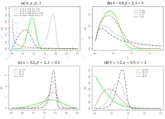
Figure 1. The pdf of X.

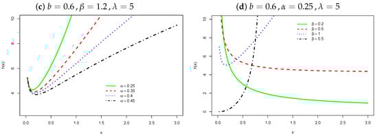
Figure 2. The hrf of X.

3. Properties

3.1. Quantile Function

By inverting (4) (for $u\in (0,1)$), the qf of X (for $\alpha >0$) has the form

$$x=F^{-1}\left(u\right)={\left[{\alpha }^{-1}{\lambda }^{-1}\left({\left\{{\left[-log(1-u)\right]}^{1/b}+1\right\}}^{\alpha }-1\right)\right]}^{1/\beta }.$$

(6)

Plots of the Bowley skewness (b) [23] and Moors kurtosis (M) [24] of X (based on quantiles) are displayed in Figure 3 and Figure 4, respectively.

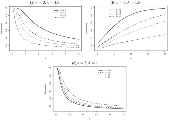
Figure 3. Skewness of X.

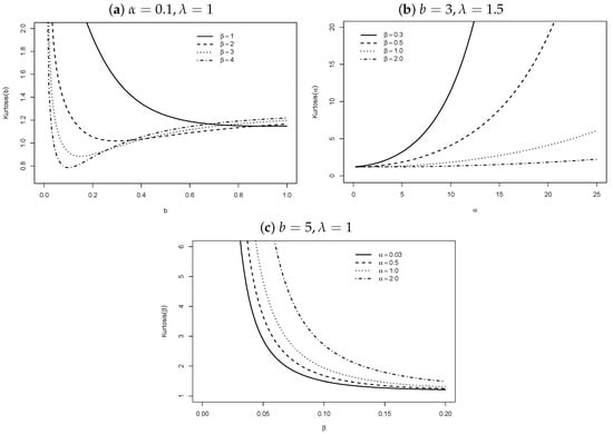
Figure 4. Kurtosis of X.

In Figure 3a, the skewness B decreases (for fixed $\beta$) when b grows. In Figure 3b, B increases to $\beta =0.5$ when $\alpha$ increases, but for larger values of $\beta$ fixed, it tends to become constant. In Figure 3c, B decreases (for any $\alpha$) when $\beta$ grows.

In Figure 4a, the kurtosis M decreases for $\beta =1$ if b grows. For high values of $\beta$ (fixed), M drops drastically when b grows, and after that, this curvature will be reversed, and then, M increases when b grows. In Figure 4b, as the parameter $\alpha$ increases, M is increasing for $\beta =0.3$, $\beta =0.5$ and $\beta =1$, and it tends to become constant for $\beta =2$. In Figure 4c, M decreases for any $\alpha$ when $\beta$ grows.

3.2. Linear Representation

In Appendix A, it is given a linear representation for the WEW pdf, namely

$$\begin{array}{c}\hfill f\left(x\right)=\left\{\begin{array}{cc}\sum _{i=0}^{\infty }{\mathrm{e}}_i\left(b\right)g(x;{\alpha }_i^{★},\beta ,{\lambda }_i^{★})\hfill & ,\mathrm{if}\alpha >0,\hfill \\ \sum _{i=0}^{\infty }{\mathrm{e}}_i\left(b\right)g(x;\beta ,{\lambda }_i^{★})\hfill & ,\mathrm{if}\alpha =0,\hfill \end{array}\right.\end{array}$$

(7)

where (for $i\ge 0$) ${\alpha }_i^{★}={(i+1)}^{-1}\alpha$, ${\lambda }_i^{★}=(i+1)\lambda$,

$$\begin{array}{c}\hfill {\mathrm{e}}_i\left(b\right)=\frac{{(-1)}^i}{(i+1)}\sum _{j,k=0}^{\infty }[(k+1)b+j]\left(\genfrac{}{}{0pt}{}{(k+1)b+j-1}{i}\right)p_{j,k}\left(b\right)\end{array}$$

and

$$\begin{array}{c}\hfill p_{j,k}\left(b\right)=\frac{{(-1)}^{j+k}b}{\left[\right(k+1)b+j]k!}\left(\genfrac{}{}{0pt}{}{-\left[\right(k+1)b+1]}{j}\right).\end{array}$$

In conclusion, this representation is important since complete and incomplete moments, generating function, mean deviations, and reliability of X can be determined from those of the EW distribution.

3.3. Moments

We can study some important characteristics of the distribution through moments.

It follows from Equations (2), (A5) and (A6)

$$\begin{array}{c}\hfill {\mu }_r^{\prime }=E\left(X^r\right)=\left\{\begin{array}{cc}{\displaystyle \frac{1}{{\lambda }^{r/\beta }{\alpha }^{r/\beta +1}}}{\displaystyle \sum _{i=0}^{\infty }}(i+1){\mathrm{e}}_i\left(b\right)B(r/\beta +1,1+i/\alpha -r/\beta ),\hfill & \mathrm{if}\alpha >0\mathrm{and}r<\beta /\alpha ,\hfill \\ {\displaystyle \frac{\Gamma (r/\beta +1)}{{\lambda }^{r/\beta }}}{\displaystyle \sum _{i=0}^{\infty }}{\displaystyle \frac{{\mathrm{e}}_i\left(b\right)}{{(i+1)}^{r/\beta }}},\hfill & \mathrm{if}\alpha =0.\hfill \end{array}\right.\end{array}$$

(8)

It is simple to verify from Equations (3), (A5) and (A6) that $T_r\left(x\right)$ can be expressed as

$$\begin{array}{c}\hfill T_r\left(x\right)=\left\{\begin{array}{cc}\frac{\beta x^{r+\beta }}{r+\beta }{\displaystyle \sum _{i=0}^{\infty }}{\mathrm{e}}_i\left(b\right){\lambda }_i^{★}{}_2{F}_1(1/{\alpha }_i^{★}+1,r/\beta +1;r/\beta +2,-{\alpha }_i^{★}{\lambda }_i^{★}{x}^{\beta }),\hfill & \mathrm{if}\alpha >0,\hfill \\ {\lambda }^{-r/\beta }{\displaystyle \sum _{i=0}^{\infty }}\frac{{\mathrm{e}}_i\left(b\right)}{{(i+1)}^{r/\beta }}\gamma (r/\beta +1,(i+1)\lambda x^{\beta }),\hfill & \mathrm{if}\alpha =0.\hfill \end{array}\right.\end{array}$$

(9)

We can obtain the mean deviations and Lorenz and Bonferroni curves from the first incomplete moment.

4. Estimation

Let $x_1,\cdots ,x_n$ be a sample of size n from (5). The log-likelihood function for $\mathit{\theta }$$={(b,\alpha ,\beta ,\lambda )}^{\top }$ from this sample reduces to

$$\begin{array}{c}\hfill l\left(\mathit{\theta }\right)=\left\{\begin{array}{c}nln\left(b\lambda \beta \right)+(\beta -1)\sum _{i=1}^{n}ln\left(x_i\right)+\left(\frac{1}{a}-1\right)\sum _{i=1}^{n}ln(1+\alpha \lambda x_i^{\beta })\hfill \\ +(b-1)\sum _{i=1}^{n}ln\left[{(1+\alpha \lambda x_i^{\beta })}^{\frac{1}{\alpha }}-1\right]-\sum _{i=1}^n{\left[{(1+\alpha \lambda x_i^{\beta })}^{\frac{1}{\alpha }}-1\right]}^b,\hfill & \alpha >0,\hfill \\ \\ nln\left(b\lambda \beta \right)+(\beta -1)\sum _{i=1}^{n}ln\left(x_i\right)+\lambda \sum _{i=1}^n{x}_i^{\beta }\hfill \\ +(b-1)\sum _{i=1}^{n}ln\left({\mathrm{e}}^{\lambda x^{\beta }}-1\right)-\sum _{i=1}^n{\left({\mathrm{e}}^{\lambda x^{\beta }}-1\right)}^b,\hfill & \alpha =0.\hfill \end{array}\right.\end{array}$$

(10)

Equation (10) for $\alpha =0$ gives the log-likelihood for the WW distribution. The maximum likelihood estimates (MLEs) can be found by maximizing $l\left(\mathit{\theta }\right)$ using the AdequecyModel library [25] of the R software; another option is the maxLik function via the maxLik library that provides a convenient interface for the MLEs [26], or by the optim function by selecting an optimization method, for example, BFGS, CG, and SANN, and still finding the Hessian matrix. We also can maximize (10) numerically using SAS (PROCNLMIXED) or the Ox program (sub-routine MaxBFGS), among others. The score components in $U\left(\mathit{\theta }\right)={(U_b,U_{\alpha },U_{\beta },U_{\lambda })}^{\top }$ (for $\alpha >0$) are reported in Appendix A.

5. Simulation Study

5.1. Simulations for the WEW Distribution

A Monte Carlo simulation study was conducted, using the BFGS algorithm in R software, to examine the accuracy of the MLEs of the parameters of X. Here, 1000 replications (for $n=50$, 100 and 300) were generated from Equation (6), where $u\sim U(0,1)$. The scenarios under study were: $b=2$, $\alpha =3$, $\beta =0.2$ and $\lambda =2$ (Setup 1—decreasing density curve; see Figure 1a); $b=1.2$, $\alpha =0.5$, $\beta =1.5$ and $\lambda =2$ (Setup 2—unimodal density curve; see Figure 1d); and $b=1.5$, $\alpha =0.2$, $\beta =2$ and $\lambda =0.2$ (Setup 3—platykurtic unimodal density curve; see Figure 1c).

We calculated the average estimates, biases and mean squared errors (MSEs) in Table 1. The biases and MSEs decrease when n grows. Thus, the estimators are consistent.

Table 1. Monte Carlo results from the WEW distribution.

Setup	n	Measures	Parameter Estimates
			$\widehat{\mathit{b}}$	$\widehat{\mathit{\alpha }}$	$\widehat{\mathit{\beta }}$	$\widehat{\mathit{\lambda }}$
Setup 1	50	Average	2.03267	2.98179	0.20299	2.02287
		Bias	0.03267	−0.01821	0.00299	0.02287
		MSE	0.04941	0.04932	0.00045	0.06756
	100	Average	2.01558	2.99028	0.20151	2.01283
		Bias	0.01558	−0.00972	0.00151	0.01283
		MSE	0.02465	0.02589	0.00023	0.03369
	300	Average	2.00696	2.99687	0.20069	2.00307
		Bias	0.00696	−0.00313	0.00069	0.00307
		MSE	0.00744	0.00804	0.00007	0.01034
Setup 2	50	Average	1.21948	0.47649	1.51371	2.02313
		Bias	0.01948	−0.02351	0.01371	0.02313
		MSE	0.01777	0.02442	0.02199	0.03930
	100	Average	1.20934	0.48818	1.50555	2.01248
		Bias	0.00934	−0.01182	0.00555	0.01248
		MSE	0.00888	0.01274	0.01110	0.01989
	300	Average	1.20425	0.49639	1.50327	2.00351
		Bias	0.00425	−0.00361	0.00327	0.00351
		MSE	0.00268	0.00391	0.00343	0.00607
Setup 3	50	Average	1.52451	0.20046	2.01178	0.20156
		Bias	0.02451	0.00046	0.01178	0.00156
		MSE	0.02781	0.01019	0.00669	0.00019
	100	Average	1.51158	0.19826	2.00618	0.20091
		Bias	0.01158	−0.00174	0.00618	0.00091
		MSE	0.01386	0.00629	0.00345	0.00010
	300	Average	1.50532	0.19738	2.00210	0.20024
		Bias	0.00532	−0.00262	0.00210	0.00024
		MSE	0.00418	0.00258	0.00105	0.00003

5.2. Misspecification Study

We investigated the behavior of the MLEs of the parameters in the WEW distribution when it was poorly specified by carrying out Monte Carlo simulations based on 1000 replications (for n = 100). The observations were simulated by taking $b=0.8$, $\alpha =3$, $\beta =2$ and $\lambda =3$. We used the maxLik library with the SANN method for each generated data set. In Table 2, the observed values are generated from the Gamma Extended Weibull (GEW) distribution [27] by taking $a=0.8$, $\alpha =3$, $\beta =2$, and $\lambda =3$. In Table 3, the observed values are generated from the EW distribution by setting $\alpha =3$, $\beta =2$, and $\lambda =3$. Further, in Table 4, the observed values are generated from the WW distribution with $b=0.8$, $\beta =2$, and $\lambda =3$.

Table 2. Simulation results for the GEW distribution when $n=100$, $a=0.8$, $\alpha =3$, $\beta =2$ and $\lambda =3$.

Measures	GEW				WEW
	$\widehat{\mathit{a}}$	$\widehat{\mathit{\alpha }}$	$\widehat{\mathit{\beta }}$	$\widehat{\mathit{\lambda }}$	$\widehat{\mathit{b}}$	$\widehat{\mathit{\alpha }}$	$\widehat{\mathit{\beta }}$	$\widehat{\mathit{\lambda }}$
AE	0.87210	2.70781	1.90117	2.83293	0.45019	3.57155	2.56222	1.93563
RB	0.09013	−0.09739	−0.04942	−0.05569	−0.43727	0.19052	0.28111	−0.35479
MSE	0.07144	0.76318	0.15322	0.70072	0.13051	1.20897	1.24062	2.55440
	GD = 317.80	AIC = 325.80	BIC = 336.23		GD = 324.63	AIC = 332.63	BIC = 343.05

Table 3. Simulation results for the EW distribution when $n=100$, $\alpha =3$, $\beta =2$ and $\lambda =3$.

Measures	EW			WEW
	$\widehat{\mathit{\alpha }}$	$\widehat{\mathit{\beta }}$	$\widehat{\mathit{\lambda }}$	$\widehat{\mathit{b}}$	$\widehat{\mathit{\alpha }}$	$\widehat{\mathit{\beta }}$	$\widehat{\mathit{\lambda }}$
AE	2.78619	1.92886	2.70198	0.42719	3.68045	2.66419	0.96509
RB	−0.07127	−0.03557	−0.09934	−0.46601	0.22682	0.33209	−0.67830
MSE	0.35906	0.06943	0.67297	0.14912	2.06455	2.12803	6.32109
	GD = 403.81	AIC = 409.81	BIC = 417.62	GD = 413.92	AIC = 421.92	BIC = 432.34

Table 4. Simulation results for the WW distribution when $n=100$, $b=0.8$, $\beta =2$ and $\lambda =3$.

Measures	WW				WEW
	$\widehat{\mathit{b}}$	$\widehat{\mathit{\beta }}$	$\widehat{\mathit{\lambda }}$		$\widehat{\mathit{b}}$	$\widehat{\mathit{\alpha }}$	$\widehat{\mathit{\beta }}$	$\widehat{\mathit{\lambda }}$
AE	0.97181	1.87195	2.86490		0.88528	0.08921	1.97642	3.11492
RB	0.21476	−0.06402	−0.04503		0.10660	−0.97026	−0.01179	0.03831
MSE	0.21604	0.24648	0.60125		0.07788	8.50249	0.09583	0.22338
	GD = −51.86948	AIC = −45.86948	BIC = −38.05397		GD = −51.78366	AIC = −43.78366	BIC = −33.36298

In addition to the average estimates (AEs), the relative biases (RB), and MSEs, we present the mean measures of global deviance (GD), say $GD=-2l\left(\widehat{\mathit{\theta }}\right)$, where $l\left(\widehat{\mathit{\theta }}\right)$ is the maximized log-likelihood function (10), AIC and BIC. They indicate that there are small sample biases in the parameter estimation. The average measures of GD, AIC and BIC for the estimated WEW distribution are very close to those values obtained from the true distributions used in the generation of the observed values. Hence, the WEW distribution provides consistent MLEs even when the data are generated from different distributions.

Clearly, the goodness-of-fit measures (GD, AIC, and BIC) are lower for the distribution from which the data are generated.

6. The LWEW Regression Model

If X has the WEW pdf (5), then $Y=log\left(X\right)$ has the log-Weibull extended Weibull (LWEW) pdf (with real support) reparameterized in terms of $\sigma ={\beta }^{-1}$ and $\mu =-\sigma log\left(\lambda \right)$, which can be expressed as (for $y\in \mathbb{R}$)

$$\begin{array}{ccc}\hfill f\left(y\right)& =& \left\{\begin{array}{c}\frac{b}{\sigma }exp\left(\frac{y-\mu }{\sigma }\right){\left[1+\alpha exp\left(\frac{y-\mu }{\sigma }\right)\right]}^{\left(\frac{1}{\alpha }-1\right)}{\left(\left\{{\left[1+\alpha exp\left(\frac{y-\mu }{\sigma }\right)\right]}^{1/\alpha }-1\right\}\right)}^{b-1}\hfill \\ \times exp\left(-{\left\{{\left[1+\alpha exp\left(\frac{y-\mu }{\sigma }\right)\right]}^{1/\alpha }-1\right\}}^b\right),,\mathrm{if}\alpha >0,\hfill \\ \\ \frac{b}{\sigma }exp\left\{\left(\frac{y-\mu }{\sigma }\right)+exp\left(\frac{y-\mu }{\sigma }\right)-{\left[{\mathrm{e}}^{{\mathrm{e}}^{\left(\frac{y-\mu }{\sigma }\right)}}-1\right]}^b\right\}{\left[{\mathrm{e}}^{{\mathrm{e}}^{\left(\frac{y-\mu }{\sigma }\right)}}-1\right]}^{b-1},\mathrm{if}\alpha =0,\hfill \end{array}\right.\hfill \end{array}$$

(11)

where $b,\alpha ,\sigma >0$ and $\mu \in \mathbb{R}$. For $\alpha =0$, we obtain the log-Weibull Weibull (LWW) model, where $\mu$ is a location and $\sigma$ is a scale.

The survival function of Y has the form

$$\begin{array}{c}\hfill S\left(y\right)=\left\{\begin{array}{cc}exp\left(-{\left\{{\left[1+\alpha exp\left(\frac{y-\mu }{\sigma }\right)\right]}^{1/\alpha }-1\right\}}^b\right),\hfill & \alpha >0,\hfill \\ exp\left\{-{\left[{\mathrm{e}}^{{\mathrm{e}}^{\left(\frac{y-\mu }{\sigma }\right)}}-1\right]}^b\right\},\hfill & \alpha =0.\hfill \end{array}\right.\end{array}$$

(12)

The density of $Z=(Y-\mu )/\sigma$ (for $z\in \mathbb{R}$) can be expressed as

$$\begin{array}{ccc}\hfill \pi \left(z\right)& =& \left\{\begin{array}{c}bexp\left(z\right){\left[1+\alpha exp\left(z\right)\right]}^{\left(\frac{1}{\alpha }-1\right)}{\left(\left\{{\left[1+\alpha exp\left(z\right)\right]}^{1/\alpha }-1\right\}\right)}^{b-1}\hfill \\ \times exp\left(-{\left\{{\left[1+\alpha exp\left(z\right)\right]}^{1/\alpha }-1\right\}}^b\right),\hfill & \mathrm{if}\alpha >0,\hfill \\ \\ bexp\left\{\left(z\right)+exp\left(z\right)-{\left[{\mathrm{e}}^{{\mathrm{e}}^{\left(z\right)}}-1\right]}^b\right\}{\left[{\mathrm{e}}^{{\mathrm{e}}^{\left(z\right)}}-1\right]}^{b-1},\hfill & \mathrm{if}\alpha =0.\hfill \end{array}\right.\hfill \end{array}$$

(13)

We construct a regression based on the LWEW distribution

$$y_i={\mathbf{v}}_i^{\top }\mathbf{\gamma }+\sigma z_i,i=1,\dots ,n,$$

(14)

where $z_i$ has pdf (13), $\mathbf{\gamma }={({\mathbf{\gamma }}_1,\cdots ,{\mathbf{\gamma }}_p)}^{\top }$ is the vector of coefficients, and ${\mathbf{v}}_i={(v_{i1},\cdots ,v_{ip})}^{\top }$ is the vector of covariates for the ith response $y_i$, which models the location parameter ${\mu }_i={\mathbf{v}}_i^{\top }\mathbf{\gamma }$.

Consider that F and C are groups of individuals that failed and are censored, respectively. The log-likelihood for $\mathbf{\theta }={(b,\alpha ,\sigma ,{\mathbf{\gamma }}^{\top })}^{\top }$ can be found from (13) and (14) as

$$\begin{array}{c}\hfill l\left(\mathbf{\theta }\right)=\left\{\begin{array}{c}q[ln\left(b\right)-ln\left(\sigma \right)]+{\displaystyle \sum _{i\in F}}{z}_i+(\frac{1}{\alpha }-1){\displaystyle \sum _{i\in F}}ln[1+\alpha exp\left(z_i\right)]\hfill \\ +(b-1){\displaystyle \sum _{i\in F}}ln\{{[1+\alpha exp\left(z_i\right)]}^{\frac{1}{a}}-1\}-{\displaystyle \sum _{i\in F}}{\left\{{\left[1+\alpha exp\left(z_i\right)\right]}^{\frac{1}{a}}-1\right\}}^b\hfill \\ -(n-q){\displaystyle \sum _{i\in C}}{\left\{{\left[1+\alpha exp\left(z_i\right)\right]}^{\frac{1}{a}}-1\right\}}^b,\hfill & \mathrm{if}\alpha >0,\hfill \\ \\ q[ln\left(b\right)-ln\left(\sigma \right)]+{\displaystyle \sum _{i\in F}}{z}_i+{\displaystyle \sum _{i\in F}}exp\left(z_i\right)+(b-1){\displaystyle \sum _{i\in F}}\left[{\mathrm{e}}^{{\mathrm{e}}^{\left(z_i\right)}}-1\right]\hfill \\ -{\displaystyle \sum _{i\in F}}{\left[{\mathrm{e}}^{{\mathrm{e}}^{\left(z_i\right)}}-1\right]}^b-(n-q){\displaystyle \sum _{i\in C}}{\left[{\mathrm{e}}^{{\mathrm{e}}^{\left(z_i\right)}}-1\right]}^b,\hfill & \mathrm{if}\alpha =0,\hfill \end{array}\right.\end{array}$$

(15)

where q is the number of failures, and $z_i=(y_i-{\mathbf{v}}_i^{\top }\mathbf{\gamma })/\sigma$. The MLE $\widehat{\mathbf{\theta }}$ of $\mathbf{\theta }$ can be found by maximizing (15).

Regression Simulation Study

A simulation study was conducted using the BFGS algorithm in R to examine the accuracy of the MLEs of the LWEW regression model with parameters: ${\gamma }_0=2.2$, ${\gamma }_1=1.2$, $\sigma =1.5$, $b=2$ and $\alpha =5$. We considered 1000 Monte Carlo replications for $n=30$, 50, and 100, and censoring percentages 0%, 10%, 30%, and 66% generated using the inverse transformation method. Occurrences of the Bernoulli distribution with success probability $(1-p)$ are generated to obtain the censored observations, where p is the percentage of censoring. The location parameter is $\mu ={\gamma }_0+{\gamma }_1{v}_{i1}$, where $v_{i1}\sim U(0,1)$.

The AEs, biases, and MSEs are reported in Table 5. The biases and MSEs usually decrease when n grows. By increasing the percentage of censoring for a fixed sample size, the biases and MSEs decrease for most AEs. Thus, an improvement in the accuracy of the estimators occurs.

Table 5. Simulation from the LWEW regression.

		0%			10%			30%			66%
n	$\mathit{\theta }$	AE	Bias	MSE	AE	Bias	MSE	AE	Bias	MSE	AE	Bias	MSE
30	${\gamma }_0$	1.98554	−0.21446	0.10958	2.09407	−0.10593	0.03849	2.16869	−0.03130	0.00769	2.20960	0.00960	0.00148
	${\gamma }_1$	1.06941	−0.13059	0.05171	1.12913	−0.07087	0.01766	1.16661	−0.03339	0.00693	1.19417	−0.00584	0.00250
	$\sigma$	1.39258	−0.10742	0.02325	1.42713	−0.07287	0.01376	1.46657	−0.03343	0.00507	1.50063	0.00063	0.00039
	b	2.18727	0.18727	0.14973	2.14912	0.14912	0.15342	2.08567	0.08567	0.16614	1.80592	−0.19408	0.24300
	$\alpha$	4.69906	−0.30094	0.18924	4.82055	−0.17945	0.08954	4.92641	−0.07359	0.02758	4.99624	−0.00376	0.00266
50	${\gamma }_0$	2.02365	−0.17635	0.07261	2.10670	−0.09329	0.02854	2.18128	−0.01872	0.00540	2.21726	0.01726	0.00119
	${\gamma }_1$	1.06815	−0.13185	0.04892	1.12879	−0.07120	0.01746	1.16988	−0.03012	0.00597	1.20095	0.00095	0.00186
	$\sigma$	1.41518	−0.08482	0.01462	1.44859	−0.05141	0.00718	1.48528	−0.01472	0.00147	1.50512	0.00512	0.00024
	b	2.13162	0.13162	0.09915	2.08522	0.08522	0.08843	1.98223	−0.01777	0.09353	1.69623	−0.30377	0.20879
	$\alpha$	4.77274	−0.22726	0.11073	4.87189	−0.12811	0.04676	4.96244	−0.03756	0.00981	5.00989	0.00989	0.00159
100	${\gamma }_0$	2.07334	−0.12666	0.03879	2.13691	−0.06309	0.01487	2.18932	−0.01068	0.00339	2.22547	0.02547	0.00118
	${\gamma }_1$	1.07318	−0.12682	0.03952	1.13136	−0.06864	0.01566	1.17634	−0.02366	0.00460	1.20802	0.00802	0.00148
	$\sigma$	1.44380	−0.05619	0.00698	1.46945	−0.03055	0.00312	1.49265	−0.00735	0.00084	1.50846	0.00846	0.00019
	b	2.07202	0.07202	0.04654	2.01271	0.01271	0.03918	1.94392	−0.05608	0.04744	1.61877	−0.38123	0.20287
	$\alpha$	4.84402	−0.15598	0.05467	4.91633	−0.08367	0.02133	4.97571	−0.02429	0.00563	5.02050	0.02050	0.00127

Clearly, it is not possible to note the same behavior for b. This can be explained, probably, because the estimators are naturally biased since the likelihood function in the presence of censoring has the contribution of the survival function.

7. Applications

7.1. The WEW Distribution

Consider a data set from the City of São Paulo (Brazil) obtained from the Severe Acute Respiratory Syndrome on the platform of the Ministry of Health (BD-SRAG at https://opendatasus.saude.gov.br/dataset/srag-2021-a-2023, accessed on: 26 May 2022), which comprises events from 31 December 2021 to March 2022. The data set passed for a filter process to obtain the 162 times (measured in days) of influenza patients from the date of admission to the hospital until cure.

In this application, we fit the WEW distribution and compared it with some special cases and competitive four-parameter distributions: GEW [27], KwW [28], BW [29], Beta Exponentiated Exponential (BEE) [30], Kumaraswamy–Gama (KwGa) [31], and Beta–Gama (BGa) [32].

The MLEs and their standard errors (SEs between parentheses) found via the SANN method (with AdequacyModel, GenSA and MASS libraries from R software) are reported in Table 6. We adopted the well-known $W^{*}$, $A^{*}$ and KS statistics (with abbreviations in place of full names) to compare the WEW distribution with some competitive distributions. We used AIC, CAIC, and BIC to compare the new distribution with some special cases. The findings are reported in Table 7. Further, the likelihood ratio (LR) in Table 6 confirms the superiority of the WEW distribution for these data.

Table 6. Estimation results.

Distribution	MLEs and SEs
WEW	b	$\alpha$	$\beta$	$\lambda$
	1.70438	96.73585	31.03260	10.76439
	(0.099237)	($8.4\times {10}^{-6}$)	(0.08398)	(0.00049)
EW *	b	$\alpha$	$\beta$	$\lambda$
	1	201.7701	81.91429	0.05117
	(-)	(0.89550)	(0.08389)	($8.4\times {10}^{-6}$)
WW **	b	$\alpha$	$\beta$	$\lambda$
	100	0	0.00838	0.68115
	(0.08579)	(-)	(0.00018)	($2.6\times {10}^{-6}$)
WE ***	b	$\alpha$	$\beta$	$\lambda$
	0.78267	0	1	0.06627
	(0.04885)	(-)	(-)	(0.00425)
GEW	a	$\alpha$	$\beta$	$\lambda$
	14.96657	0.49719	2.19879	90.77049
	(0.00805)	(0.00503)	(0.00304)	($5.9\times {10}^{-5}$)
KwW	a	b	$\beta$	$\lambda$
	4.39908	102.1187	0.33391	98.50308
	(0.28679)	(0.00061)	(0.03279)	($6.2\times {10}^{-6}$)
BW	a	b	$\beta$	$\lambda$
	0.52781	185.9165	1.90579	211.1240
	(0.07526)	($8.4\times {10}^{-6}$)	(0.07965)	($2.9\times {10}^{-6}$)
BEE	a	b	$\lambda$	$\alpha$
	7.90232	0.33214	0.50962	0.24477
	(1.22239)	(0.02937)	(0.00034)	(0.00008)
KwGa	a	b	$\alpha$	$\beta$
	8.03469	0.24479	0.43813	0.60068
	(0.16546)	(0.01926)	($1.8\times {10}^{-5}$)	($1.8\times {10}^{-5}$)
BGa	a	b	$\alpha$	$\beta$
	0.03100	0.19168	40.77195	2.31482
	($2.8\times {10}^{-6}$)	($6.3\times {10}^{-6}$)	($7.7\times {10}^{-7}$)	($1.8\times {10}^{-6}$)

* $LR$ = 29.373; (p-value ≤ 0.0001); ** $LR$ = 35.165; (p-value ≤ 0.0001); *** $LR$ = 83.863; (p-value ≤ 0.0001).

Table 7. GoF statistics for some fitted models.

Distribution	AIC	CAIC	BIC	${\mathit{W}}^{*}$	${\mathit{A}}^{*}$	K-S	K-S p-Value
WEW	945.8351	946.0899	958.1855	0.15721	1.21619	0.08724	0.1698
EW	973.2082	973.3601	982.4710	0.40638	3.32898	0.24370	$8.8\times {10}^{-9}$
WW	979.0003	979.1522	988.2631	0.50182	3.08837	0.11898	0.02038
WE	1025.698	1025.773	1031.873	1.01694	6.03306	0.18871	$1.9\times {10}^{-5}$
GEW	952.3737	952.6284	964.7241	0.16684	1.32491	0.09982	0.07925
KwW	972.5957	972.8505	984.9461	0.40059	2.48240	0.11419	0.02927
BW	1011.977	1012.232	1024.328	0.91635	5.48942	0.16400	0.00033
BEE	960.2507	960.5055	972.6011	0.25811	1.64087	0.12340	0.01439
KwGa	958.1527	958.4075	970.5031	0.23330	1.49163	0.13183	0.00717
BGa	977.6345	977.8893	989.9849	0.35983	2.22311	0.16333	0.00035

Further, we compared the proposed distribution with the previous models via the generalized likelihood ratio (GLR) test [33]. The results in Table 8 indicate that the WEW distribution is the most suitable model. The histogram and the best four fitted pdfs are displayed in Figure 5a. Figure 5b reports the empirical and estimated cdfs. They also reveal the superiority of the WEW distribution.

Table 8. GLR tests for some fitted models.

Distribution	$\mathit{GLR}$ Statistic	Decision
WEW × GEW	7.70553	WEW is chosen
WEW × KwW	18.80256	WEW is chosen
WEW × BW	6.01989	WEW is chosen
WEW × BEE	9.14457	WEW is chosen
WEW × KwGa	10.50785	WEW is chosen
WEW × BGa	11.25128	WEW is chosen

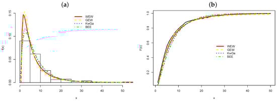
Figure 5. (a) Estimated densities. (b) Empirical and estimated cdfs.

7.2. The LWEW Regression Model

We used a data set from a randomized clinical trial carried out to investigate the effect of therapy with steroids in the treatment of acute viral hepatitis [34]. Twenty-nine patients with this disease were randomized to receive either a placebo (lactose) or the steroid (Methylprednisolone) treatment. Each patient was followed for 16 weeks or until death (event of interest) or even loss of follow-up (censoring). The observed survival times, in weeks, for the two groups are reported in Table 9. The explanatory variable in this work is taken as: ($v_1$): treatment (placebo = 1, steroid = 2).

Table 9. Survival times in weeks from hepatitis study.

Placebo: 1+, 2+, 3, 3, 3+, 5+, 5+, 16+, 16+, 16+, 16+, 16+, 16+,16+, 16+.

Steroid: 1, 1, 1, 1+, 4+, 5, 7, 8, 10, 10+, 12+, 16+, 16+, 16+.

Note: + indicates censoring.

We fit the LWEW regression model

$$y_i={\gamma }_0+{\gamma }_1{v}_{i1}+\sigma z_i,$$

(16)

where $z_i$ has pdf (13).

Some competing models for the regression modeling are: log-gamma extended Weibull (LGEW) [27], log-beta Weibull (LBW) [35], and log-Kumaraswamy–Weibull or Kumaraswamy Gumbel (KwGu) [36].

Table 10 provides the MLEs for the fitted LWEW, LEW, LWW, LGEW, LBW and KwGu regressions via the maxLik function and the BFGS method in R software. The codes can be accessed at https://github.com/elisangelacbiazatti/WEW (accessed on 28 April 2023). This table shows that the LWEW is the best model. The LR statistic confirms the superiority of the LWEW model for both its sub-models at the 1% level of significance. Further, control treatment and steroids are statistically different. Thus, patients who received control treatment had a shorter time to death than patients who received steroids, since the estimate of the coefficient of the treatment variable ($v_1$) is negative.

Table 10. Estimation results [p values] and adequacy measures for some regressions.

Model	MLEs, SEs and p Values					AIC	CAIC	BIC
LWEW	b	$\alpha$	$\sigma$	${\gamma }_0$	${\gamma }_1$	52.329	54.938	59.166
	0.58060	150.90603	0.03382	2.34490	−1.10239
	(0.18658)	(4.08123)	(0.01369)	(0.147361)	(0.08117)
				[<0.0001]	[<0.0001]
LEW *	b	$\alpha$	$\sigma$	${\gamma }_0$	${\gamma }_1$	107.135	108.802	112.604
	1	$7.7\times {10}^{-7}$	23.46137	11.71906	13.90735
	(-)	(0.03386)	(0.07149)	(0.02771)	0.03222
				[<0.0001]	[<0.0001]
LWW **	b	$\alpha$	$\sigma$	${\gamma }_0$	${\gamma }_1$	61.041	62.707	66.509
	0.10982	0	0.13328	6.63796	−1.86159
	(0.02451)	(-)	(0.00076)	(0.00074)	(0.00025)
				[<0.0001]	[<0.0001]
LGEW	a	$\alpha$	$\sigma$	${\gamma }_0$	${\gamma }_1$	53.225	55.834	60.061
	0.73631	169.03010	0.03457	2.32548	−1.10290
	(0.18543)	(4.20435)	(0.01646)	(0.18200)	(0.09769)
				[<0.0001]	[<0.0001]
LBW	a	b	$\sigma$	${\gamma }_0$	${\gamma }_1$	92.834	95.443	99.671
	0.08411	0.73309	0.13038	4.41069	−0.81134
	(0.01656)	(0.30395)	(0.00364)	(0.00221)	(0.00113)
				[<0.0001]	[<0.0001]
KwGu	a	b	$\sigma$	${\gamma }_0$	${\gamma }_1$	72.917	75.526	79.754
	0.04522	0.34645	0.08871	2.81745	−0.10872
	(0.01634)	(0.09152)	(0.00002)	(0.04302)	(0.04298)
				[<0.0001]	[0.01143]

* $LR$ = 56.806; (p-value = $4.8\times {10}^{-14}$); ** $LR$ = 10.711; (p value = 0.00106).

The plots of the Kaplan–Meier and estimated survival functions in Figure 6 support that the LWEW model is the best among the fitted models.

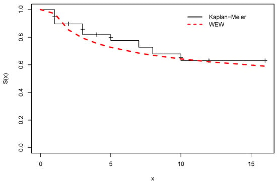
Figure 6. Kaplan–Meier and estimated survival functions.

The plot of the deviance residuals randomized around zero is reported in Figure 7a. A normal plot with an envelope is shown in Figure 7b. The model fits the data reasonably well.

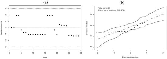
Figure 7. Deviance residuals. (a) Index plot. (b) Normal plot with envelope.

8. Conclusions

We introduced the Weibull extended Weibull density and provided some of its properties. The consistency of the maximum likelihood estimators is proven by a simulation study. An application to real influenza data revealed its flexibility. We constructed a regression model log-Weibull extended Weibull and performed some simulations to study the behavior of the estimators in small and large samples. We compared the fit to acute viral hepatitis data with other existing models and performed a residual analysis study for the final model. Overall, the two applications showed the utility of the new models for symmetric and asymmetric data, censored or uncensored. In future works, we can, for example, select other systematic components for the regression model and, as an alternative method, present the estimation of the model parameters from the Bayesian approach.

References

- Mudholkar, G.S.; Srivastava, D.K.; Kollia, G.D. A generalization of the Weibull distribution with application to the analysis of survival data. J. Am. Stat. Assoc. 1996, 91, 1575–1583. [Google Scholar] [CrossRef]
- Wienke, A. Frailty Models in Survival Analysis; Chapman and Hall/CRC: Boca Raton, FL, USA, 2011. [Google Scholar]
- Murthy, D.P.; Xie, M.; Jiang, R. Weibull Models; John Wiley & Sons: Hoboken, NJ, USA, 2004. [Google Scholar]
- Almalki, S.J.; Nadarajah, S. Modifications of the Weibull distribution: A review. Reliab. Eng. Syst. Saf. 2014, 124, 32–55. [Google Scholar] [CrossRef]
- Ishaq, A.I.; Abiodun, A.A. The Maxwell–Weibull distribution in modeling lifetime datasets. Ann. Data Sci. 2020, 7, 639–662. [Google Scholar] [CrossRef]
- Klakattawi, H.S. Survival analysis of cancer patients using a new extended Weibull distribution. PLoS ONE 2022, 17, e0264229. [Google Scholar] [CrossRef] [PubMed]
- Mudholkar, G.S.; Srivastava, D.K. Exponentiated Weibull family for analyzing bathtub failure-rate data. IEEE Trans. Reliab. 1993, 42, 299–302. [Google Scholar] [CrossRef]
- Mudholkar, G.S.; Srivastava, D.K.; Freimer, M. The exponentiated Weibull family: A reanalysis of the bus-motor-failure data. Technometrics 1995, 37, 436–445. [Google Scholar] [CrossRef]
- Bourguignon, M.; Silva, R.B.; Cordeiro, G.M. The Weibull-G family of probability distributions. J. Data Sci. 2014, 12, 53–68. [Google Scholar] [CrossRef]
- Tahir, M.H.; Cordeiro, G.M.; Mansoor, M.; Zubair, M.; Alizadeh, M. The Weibull–Dagum Distribution: Properties and Applications. Commun.-Stat.-Theory Methods 2016, 45, 7376–7398. [Google Scholar] [CrossRef]
- Ishaq, A.I.; Usman, A.; Tasi’u, M.; Aliyu, Y.; Idris, F.A. A new Weibull-Kumaraswamy Distribution: Theory and Applications. Niger. J. Sci. Res. 2017, 16, 158–166. [Google Scholar]
- Benkhelifa, L. The Weibull Birnbaum-Saunders distribution and its applications. Stat. Optim. Inf. Comput. 2021, 9, 61–81. [Google Scholar] [CrossRef]
- Hassan, A.S.; Mohamed, R.E. Weibull inverse Lomax distribution. Pak. J. Stat. Oper. Res. 2019, 15, 587–603. [Google Scholar] [CrossRef]
- Hussain, N.A.; Doguwa, S.I.S.; Yahaya, A. The Weibull-Power Lomax distribution: Properties and application. Commun. Phys. Sci. 2020, 6, 869–881. [Google Scholar]
- Biazatti, E.C.; Cordeiro, G.M.; Rodrigues, G.M.; Ortega, E.M.; de Santana, L.H. A Weibull-Beta Prime Distribution to Model COVID-19 Data with the Presence of Covariates and Censored Data. Stats 2022, 5, 1159–1173. [Google Scholar] [CrossRef]
- Chow, E.J.; Rolfes, M.A.; O’Halloran, A.; Alden, N.B.; Anderson, E.J.; Bennett, N.M.; Billing, L.; Dufort, E.; Kirley, P.D.; George, A.; et al. Respiratory and nonrespiratory diagnoses associated with influenza in hospitalized adults. JAMA Netw. Open 2020, 3, e201323. [Google Scholar] [CrossRef]
- Chow, E.J.; Rolfes, M.A.; O’Halloran, A.; Anderson, E.J.; Bennett, N.M.; Billing, L.; Chai, S.; Dufort, E.; Herlihy, R.; Kim, S.; et al. Acute cardiovascular events associated with influenza in hospitalized adults: A cross-sectional study. Ann. Intern Med. 2020, 173, 605–613. [Google Scholar] [CrossRef] [PubMed]
- Rahman, A.; Jiang, D. Regional and temporal patterns of influenza: Application of functional data analysis. Infect. Dis. Model. 2021, 6, 1061–1072. [Google Scholar] [CrossRef]
- Kauhl, B.; Heil, J.; Hoebe, C.J.P.A.; Schweikart, J.; Krafft, T.; Dukers-Muijrers, N.H.T.M. The Spatial Distribution of Hepatitis C Virus Infections and Associated Determinants—An Application of a Geographically Weighted Poisson Regression for Evidence-Based Screening Interventions in Hotspots. PLoS ONE 2015, 10, e0135656. [Google Scholar] [CrossRef]
- Konerman, M.A.; Beste, L.A.; Van, T.; Liu, B.; Zhang, X.; Zhu, J.; Sameer, D.; Saini, S.D.; Su, G.L.; Nallamothu, B.K.; et al. Machine learning models to predict disease progression among veterans with hepatitis C virus. PLoS ONE 2019, 14, e0208141. [Google Scholar] [CrossRef]
- Razavi, H.; Gonzalez, Y.S.; Yuen, C.; Cornberg, M. Global timing of hepatitis C virus elimination in high-income countries. Liver Int. 2020, 40, 522–529. [Google Scholar] [CrossRef]
- Uçar, S. Analysis of hepatitis B disease with fractal–fractional Caputo derivative using real data from Turkey. J. Comput. Appl. Math. 2023, 419, e114692. [Google Scholar] [CrossRef]
- Kenney, J.F.; Keeping, E.S. Mathematics of Statistics; D. Van Nostrand Company: Toronto, Japan, 1961; Volume 1, p. 429. [Google Scholar]
- Moors, J. A Quantile Alternative for Kurtosis. J. R. Stat. Soc. Ser. (Stat.) 1988, 37, 25–32. [Google Scholar] [CrossRef]
- Marinho, P.R.D.; Silva, R.B.; Bourguignon, M.; Cordeiro, G.M.; Nadarajah, S. AdequacyModel: An R package for probability distributions and general purpose optimization. PLoS ONE 2019, 14, e0221487. [Google Scholar] [CrossRef] [PubMed]
- Henningsen, A.; Toomet, O. maxLik: A package for maximum likelihood estimation in R. Comput. Stat. 2011, 26, 443–458. [Google Scholar] [CrossRef]
- Cordeiro, G.M.; Lima, M.D.C.; Gomes, A.E.; da-Silva, C.Q.; Ortega, E.M.M. The Gamma Extended Weibull distribution. J. Stat. Distrib. Appl. 2016, 3, 1–19. [Google Scholar] [CrossRef]
- Cordeiro, G.M.; Ortega, E.M.M.; Nadarajah, S. The Kumaraswamy Weibull distribution with application to failure data. J. Frankl. Inst. 2010, 347, 1399–1429. [Google Scholar] [CrossRef]
- Lee, C.; Famoye, F.; Olumolade, O. Beta-Weibull Distribution: Some Properties and Applications to Censored Data. J. Mod. Appl. Stat. Methods 2007, 6, 173–186. [Google Scholar] [CrossRef]
- Barreto-Souza, W.; Santos, A.H.S.; Cordeiro, G.M. The Beta Generalized Exponential distribution. J. Stat. Comput. Simul. 2010, 80, 159–172. [Google Scholar] [CrossRef]
- Cordeiro, G.M.; de Castro, M. A New Family of Generalized Distributions. J. Stat. Comput. Simul. 2011, 81, 883–898. [Google Scholar] [CrossRef]
- Kong, L.; Lee, C.; Sepanski, J. On the Properties of Beta-Gamma Distribution. J. Mod. Appl. Stat. Methods 2007, 2007 6, 187–211. [Google Scholar] [CrossRef]
- Vuong, Q.H. Likelihood Ratio Tests for Model Selection and Non-Nested Hypotheses. Econom. J. Econom. Soc. 1989, 57, 307–333. [Google Scholar] [CrossRef]
- Gregory, P.B.; Knauer, C.M.; Kempson, R.L.; Miller, R. Steroid Therapy in Severe Viral Hepatitis. N. Engl. J. Med. 1976, 294, 681–687. [Google Scholar] [CrossRef] [PubMed]
- Ortega, E.M.; Cordeiro, G.M.; Kattan, M.W. The Log-Beta Weibull Regression Model with Application to Predict Recurrence of Prostate Cancer. Stat. Pap. 2013, 54, 113–132. [Google Scholar] [CrossRef]
- Cordeiro, G.M.; Nadarajah, S.; Ortega, E.M.M. The Kumaraswamy Gumbel Distribution. Stat. Methods Appl. 2012, 21, 139–168. [Google Scholar] [CrossRef]
Disclaimer/Publisher’s Note: The statements, opinions and data contained in all publications are solely those of the individual author(s) and contributor(s) and not of MDPI and/or the editor(s). MDPI and/or the editor(s) disclaim responsibility for any injury to people or property resulting from any ideas, methods, instructions or products referred to in the content. |
© 2023 by the authors. Licensee MDPI, Basel, Switzerland. This article is an open access article distributed under the terms and conditions of the Creative Commons Attribution (CC BY) license (https://creativecommons.org/licenses/by/4.0/).