Abstract
In multifactor fixed-effects ANOVAs, we show how to construct orthonormal F contrasts for main effects. Our primary focus is the case when the levels of the factor of interest are ordered. Likewise, in multifactor equally replicated fixed-effects ANOVAs, we show how to construct orthonormal F contrasts for interactions. The primary focus here is on interactions when both factors are ordered, although the approach also applies if just one factor is ordered. Interactions with both factors ordered may be interpreted in terms of generalised correlations.
1. Introduction
In undergraduate courses and texts for users of statistics, contrasts are often seen as a means to better understand a significant main effect. Such texts include Box, Hunter and Hunter [1], Draper and Smith ([2], for example, p. 477) and Snedecor and Cochran ([3], see Section 12.8), although a more extensive account is given in ([4], Section 3.2). Most focus on the case when the levels of the factor are unordered, although ordered levels are occasionally mentioned. See, for example:
https://en.wikipedia.org/wiki/Contrast_(statistics), https://people.stat.sc.edu/grego/courses/stat706/Polynomial_Contrasts.pdf and https://www.ndsu.edu/faculty/horsley/Lncntrst.pdf, all of which were accessed on 25 August 2023.
As an example of the use of orthogonal contrasts, suppose that in an ANOVA, there are three levels of a treatment effect. Especially if this is significant, a data analyst may wish to seek information about how this effect may have arisen. Sensible comparisons may be of the control with the two other levels and of the non-control treatments.
In most sources, we have found that it is unusual to consider unbalanced designs in which there are different numbers of observations in the levels of the treatments, and it is rare for sources to provide any details when the treatment levels are ordered or to discuss contrasts for interactions. Here, guidance is given on all of these cases.
In Thas et al. [5], given treatments for which the levels are ordered, the Kruskal–Wallis, Friedman and Durbin test statistics were decomposed into orthonormal contrasts. These assessed the treatments for linear, quadratic, etc. trends. However, their development required the design to be balanced. It therefore did not directly apply to the Kruskal–Wallis test in general. This issue was resolved in Rayner and Livingston, Jr. [6], who gave a general construction for ordered treatment levels enabling test statistics to be expressed as a sum of squares of orthonormal contrasts. The squared contrasts asymptotically had distribution and are hence called χ2 contrasts.
Here, we address multifactor fixed-effects ANOVAs. We consider decomposing main effects and two-factor interactions into orthonormal contrasts, with special reference to the case when the levels of the treatments are ordered. To avoid issues with sum-of-squares types (see, for example, https://md.psych.bio.unigoettingen.de/mv/unit/lm_cat/lm_cat_unbal_ss_explained.html (accessed on 25 August 2023)), interactions are only considered for the equally replicated model. Then, the design is orthogonal, and there is only one accepted definition of the interaction sum of squares.
We decompose a main-effects sum of squares to construct orthonormal contrasts that can be assessed using the F1,edf distribution, where edf is the error degrees of freedom. These F contrasts are direct competitors to χ2 contrasts, and to the best of our knowledge, the case when the factor has ordered levels has not previously been discussed in the literature.
We then turn to constructing F contrasts for interactions between two factors, assuming an equally replicated model. The approach can be modified to interactions between more than two factors, but this is not developed here. When the levels of both factors are ordered, the F contrasts may be interpreted as generalised correlations. See, for example, Rayner and Beh [7].
For equally replicated two-way models, the traditional way to interpret interactions is subjectively, through a table of cell means. Examples are given that demonstrate that the analysis using contrasts:
- Is objective;
- Can find effects masked by non-significant effects; and
- Positively augments traditional cell mean plots.
The contrasts constructed subsequently do not require equally spaced scores. When scores are needed, they are incorporated into the construction of the orthonormal functions necessary for the construction of the contrasts. The orthonormal functions may be generated using the method of Rayner et al. [8].
2. The Construction of Orthonormal Contrasts for Main Effects in a Fixed-Effects ANOVA
We begin by defining orthonormal contrasts. Suppose Y = (Y1, …, Yt)T is a vector of random variables, and c = (c1, …, ct)T is a vector of constants. For i = 1, …, t, suppose Yi is the sum of ni observations, that n = and that pi = ni/n. Then, cTY is a contrast in Y if and only if p1c1 + … + ptct = 0.
In general, a weight function is a set {pi} in which pi > 0 for i = 1, …, t and = 1. Suppose is orthogonal (orthonormal) with weight function {pi}. Here, hu = (hu1, …, hut)T for u = 1, …, t. Orthonormality means that E[] = δuv, the Kronecker delta in which the expectation here is with respect to the distribution with probability function {pi}. It is customary to take the orthonormal function of degree zero to be identically 1, and here, ht is designated to fulfil this function.
The orthonormality and choice of ht mean that for u = 1, …, t − 1, . It follows that the = are contrasts. In full, the are said to be orthonormal contrasts with weight function {pi}. However, many users say orthogonal contrasts when they strictly mean orthonormal contrasts.
Now, consider a fixed-effects ANOVA design with multiple factors. The observations are mutually independent and normally distributed with constant variance σ2. Suppose Yij is the jth of ni observations of the ith of r levels of factor A. There are n = observations in all, and ultimately but not immediately, it is assumed that the levels of A are ordered. Write Yi. for the sum of the observations for level i and for the mean of same.
Under the null hypothesis of no factor A effect, the factor sum of squares, SSF = = − , has the distribution. Now, write Z = (, …, )T, so that Z/s is the vector of the standardised response sums for the levels of the factor A. The elements of Z/s are standard normal with, say, covariance matrix V.
Now, E[Z] = 0, and E[ZZT] = V has rank (V) = r − 1. Write W = V−0.5Z in which V− is a generalised inverse. Taking the zero eigenvalue as the rth, the covariance matrix of W to Ir−1 1. Then, SSF = ZTZ = WTVW. Since SSF is distributed as , V is idempotent with rank r − 1. It therefore has r − 1 eigenvalues 1 and one zero. Suppose the eigenvectors m1, …, mr−1 correspond to the eigenvalues of one, and mr to the eigenvalue 0; then, the singular value decomposition of V is V = . Note that using ZT1r = 0, , so that mr = 1r. Now, since V0.5 = V−0.5 = V = V−, for i = 1, …, r − 1, = = ( + … + )Z = . Thus,
As observed in Thas et al. [5] (2012, Appendix A), there is great freedom in choosing the {mu}: it is only required that m1, …, mr−1 be mutually orthonormal, and that all are orthogonal to the eigenvector corresponding to the eigenvalue one.
We now have SSF/σ2 = ZTZ/σ2 = . Using the orthogonality of the {mu}, for any u ≠ v, = 0, and from Craig’s theorem (see Craig [9]), the {} are mutually independent. Thus, for i = 1, …, r, the ()2/σ2 are mutually independent and distributed. The error sum of squares, say SSE, has the distribution, where edf is the error degrees of freedom. Since SSF is independent of ESS, so are its squared contrasts. It follows that the ()2/{SSE/edf} = Fu, say, are mutually independent and F1,edf distributed. In the Fu, the error variance is not explicitly required.
To choose the {mu}, first suppose h1, …, ht are orthonormal with weight function {pi}, so that . Put mui = . Then, (mui) is an orthogonal matrix, and the are orthonormal contrasts. For ordered treatments, the {hu} may be chosen to be the orthonormal polynomials on the weight function (n1/n, …, nr/n)T with the degree zero polynomial identically one. We call the resulting contrasts ordered F contrasts. When the treatment levels are not ordered, the scenario will suggest which comparisons are of interest. However, a fallback is to use a Helmert matrix, for which see Lancaster [10]. Examples are given in Rayner and Livingston, Jr. [6]. Note that our treatment allows for unbalanced treatment levels.
It may be that the factor effect is significant at a predetermined level of significance, and hence, that the factor-level means are not statistically consistent. If the levels of the factor are ordered, analysis of the ordered F contrasts may indicate how the level means are different. A statistically significant degree one contrast indicates a linear effect, a statistically significant degree two contrast indicates an independent quadratic effect, and so on. These are objective assessments, and though a plot of means against levels may suggest certain polynomial effects, plots only provide a subjective assessment. A scenario of perhaps more interest occurs when a main effect is not statistically significant, but one or more orthonormal contrasts are. Thus, the omnibus main effect masks effects that may be interesting and important. Failure to examine the contrasts means that such effects are not found.
We are mindful of the issue of data dredging: applying multiple tests to the one data set. We expect the main application of these contrasts is in exploratory data analysis. However, if previous analysis suggests there may be, say, quadratic effects, then the quadratic contrast may be used directly.
3. The Construction of Orthonormal Contrasts for Fixed-Effects ANOVA Interactions
We now consider interaction effects. The model is assumed to be a multifactor fixed-effects ANOVA, but we focus only on two factors, say, A and B. Suppose Yijk is the kth of nij observations of the ith of r levels of factor A and the jth of c levels of factor B. The levels of both A and B will ultimately but not immediately be assumed to be ordered. All observations are mutually independent and normally distributed with constant variance σ2.
It is assumed that nij = l > 1 for all i and j, so that there are n = lrc observations in all. The equally replicated design is orthogonal, so there is no issue with sum-of-squares types. The error degrees of freedom are edf = (l − 1)rc.
Write for the mean of the observations for level i of factor A and level j of factor B, for the mean of the observations for level i of factor A, for the mean of the observations for level j of factor B and for the mean of all of the observations. As, for example, in Kuehl ([4], p. 185), the interaction sum of squares is:
Without loss of generality, assume the observations have zero means, so that the are IN(0, ) distributed. Write:
in which .
Z = (Z11, …, Z1c, Z21, …, Z2c, …, Zr1, …, Zrc)T
Now, Y/s is distributed as Nrc(0, Irc) and SSAB = ZTZ in which, say, E[Z] = 0, and cov(Z) = V. Since SSAB has the distribution and rank(V) = (r − 1)(c − 1), then, as in the previous section, we may express SSAB/σ2 as ZTZ/σ2 = . Here, {ms} are eigenvectors of V, and it is only necessary to specify those corresponding to the non-zero eigenvalues of one. As previously, there is great flexibility in the choice of m1, …, m(r−1)(c−1). Using the orthogonality of the {ms}, for any s ≠ s′, = 0 and from Craig’s theorem, the {} are mutually independent. Thus, for s = 1, …, (r − 1)(c − 1), the ()2 are mutually independent and distributed. The sum of squares, SSE, has the distribution and is independent of the treatment sum of squares, and hence its squared contrasts. It follows that the ()2/{SSE/edf} = Fs, say, are mutually independent and F1,edf distributed.
We now show how the {ms} may be constructed. Suppose D is any r × r idempotent matrix of rank r − 1, and E is any c × c idempotent matrix of rank c − 1. Then, D has r − 1 eigenvalues one and one zero, and E has c − 1 eigenvalues one and one zero. It follows that D ⊗ E is idempotent and has (r − 1)(c − 1) eigenvalues one and r + c − 1 eigenvalues zero. In particular, suppose the eigenvectors of D corresponding to the eigenvalue one are d1, …, dr−1 (with dr = 1r), and the eigenvectors of E corresponding to the eigenvalue one are e1, …, ec−1 (with ec = 1c). Then, the eigenvectors du ⊗ ev, u = 1, …, r − 1 and v = 1, …, c − 1 of D ⊗ E corresponding to the eigenvalues of 1 are mutually orthonormal.
The singular value decomposition of V gives V = in which ms = du ⊗ ev, where s indexes (u, v), u = 1, …, r − 1 and v = 1, …, c − 1. The F orthonormal contrasts Fs = ()2/{SSE/edf} of the interaction are now fully specified. We say the contrast corresponding to a particular choice of u and v is of degree (u, v). In practice, {du} and {ev} could be chosen to be based on the orthonormal polynomials when the levels of the factor are ordered or, for example, the Helmert matrix when they are not.
4. Generalised Correlations
We turn now to the choice and interpretation of the ordered F interaction contrasts. As a prelude, suppose we have an r × c table of counts {Nij}. Further, suppose {au} is orthonormal on {}, and {bv} is orthonormal on {}. It was shown in Rayner and Best ([11], Section 8.2) that given an appropriate smooth model, if Vuv = , then is a score test statistic for testing if the (u, v)th generalised correlation is consistent with being zero. Generalised correlations are defined and discussed in Rayner and Beh [7]. Also see Rayner and Livingston, Jr. ([12], Section 6.3). Under the null hypothesis of independence, the Vuv are asymptotically independent and asymptotically standard normal.
To access the interpretation of generalised correlations, suppose that in the previous section, the levels of both factors are ordered, and we choose {au} to be orthonormal polynomials with weight function {pi} and at = 1r, and we choose {bv} to be orthonormal polynomials with weight function {qj} and bt = 1c. Write msij = , where s is the index corresponding to a particular (u, v) couple. Since we are assuming an equally weighted design here, pi = 1/r, qj = 1/c, and msij = .
We have called the ordered F interaction contrast of degree (u, v) in which a typical element of Z is (. In more detail, this contrast is in which, since au = (au1, …, aur)T and bv = (bv1, …, bvc)T,
Thus, is given by:
Apart from a scale factor, the typical ordered F interaction contrast is . This is of the same form as Vuv, and hence the degree (u, v) F contrast may be interpreted as testing for the (u, v)th generalised correlation.
Generalised correlations of degree (1, v) and (u, 1) are interpreted as polynomial effects of degree u (or v) in one variable as the other variable increases. In particular, generalised correlations of degree (1, 2) and (2, 1) are interpreted as umbrella effects: as one variable increases, the other variable either increases then decreases or decreases then increases. Other generalised correlations are harder to interpret, which is one reason why we do not proceed to analysing three (and more)-factor interactions.
If all the ordered F interaction contrasts are consistent with being zero, a reasonable conclusion is that the responses for any level of one factor are independent/not affected by the levels of the other factor. If any ordered F interaction contrast is not consistent with being zero, then these levels are not independent of each other, and there is a significant interaction effect. Ordered F interaction contrasts and cell mean plots are different tools for assessing interaction effects, and it should be expected that they will give similar but not necessarily identical interpretations of the data.
5. Examples
In the examples following the design is a replicated two-factor ANOVA in which the levels of both factors are ordered. In each, we begin with the usual analysis, calculating the main effects and interaction p-values. Then, to give subjective insights to the main effects, for each factor, plots are given of the response means against the factor levels. To give subjective insights for the interaction effect, for each main effect, plots are given of cell means against levels of the main effect. Smoothers connect the responses for each level of the other main effect to highlight how the levels of the other main effect vary. All this is, of course, standard.
It is helpful to reflect upon what these plots do and do not do. Underpinning them is a three-dimensional plot of responses against the levels of each factor. The main effects plots aggregate over one factor, giving two-dimensional projections. The interaction plots take slices for each level of one factor and aggregate them on single two-dimensional plots. As such, they ignore the fact that that factor is ordered: it is being treated as unordered.
For the main effects analyses, the contrasts are isolating linear, quadratic, etc. effects, and these are often subjectively apparent on the plots.
For the interaction analysis, the ordered interaction contrasts are isolating complex effects on the surface of the three-dimensional plot of responses against the levels of each factor. For example, a ridge corresponding to the x-y line would be reflected by a significant (1, 1) interaction. The ordered interaction contrasts utilise the fact that the levels of both factors are ordered and give objective rather than subjective assessments.
Wireworm data. The data in Table 1 are the number of wireworms in soil samples from a randomised block experiment on the effects of two fumigants, C and S; O is a control. There were four samples per plot and five blocks. See Snedecor and Cochran ([3] p. 266), who reference Ladell [13]. Subsequently, both factors are assumed to be ordered, and natural scores are used. R output for the ANOVA follows.
| Analysis of Variance Table | |||||
| Response: response | |||||
| Df | Sum Sq | Mean Sq | F value | Pr (>F) | |
| fum | 2 | 293.4 | 146.72 | 16.113 | 5.28 × 10⁻⁶ *** |
| block | 4 | 151.2 | 37.79 | 4.150 | 0.00603 ** |
| fum:block | 8 | 196.2 | 24.53 | 2.694 | 0.01641 * |
| Residuals | 45 | 409.8 | 9.11 | ||

Table 1.
Counts of wireworms in fumigated soil.
Subsequently, p-values in parentheses are permutation test p-values based on 1,000,000 permutations using method 1 of Manly ([14] p. 145). It will be seen that there is good agreement between the p-values using the F distribution and permutation testing.
From the ANOVA, the fumigant p-value is 0.0000 (0.0000) on two degrees of freedom, the block p-value is 0.0060 (0.0194) on four degrees of freedom, and the interaction p-value is 0.0164 (0.0158) on eight degrees of freedom. See Figure 1 and Figure 2.
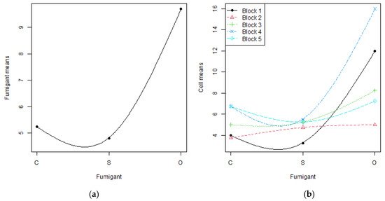
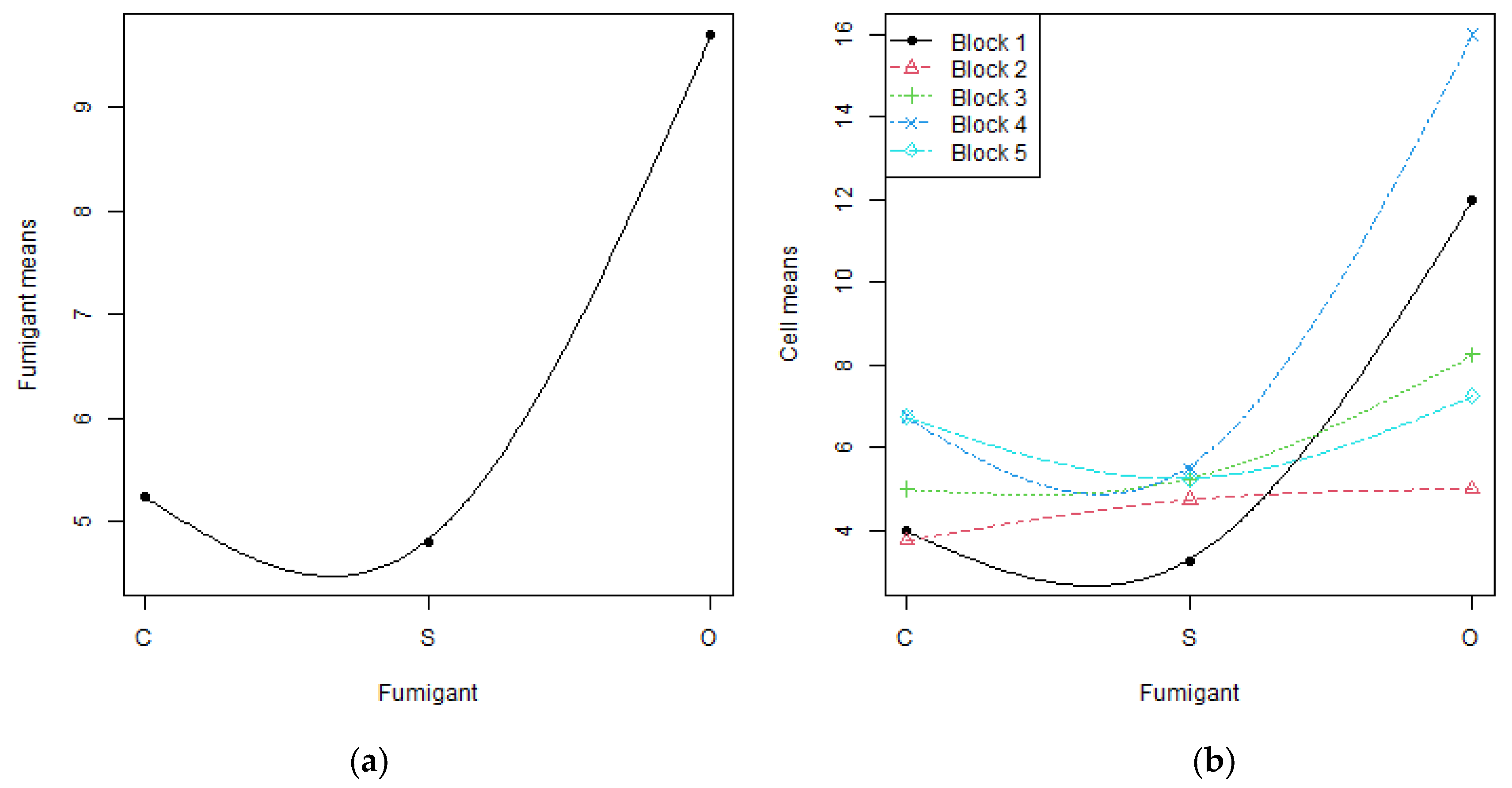
Figure 1.
Plots of (a) fumigant means and (b) cell means versus fumigants.
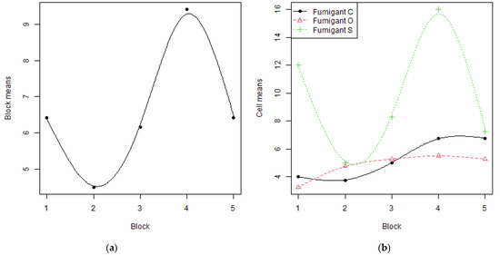
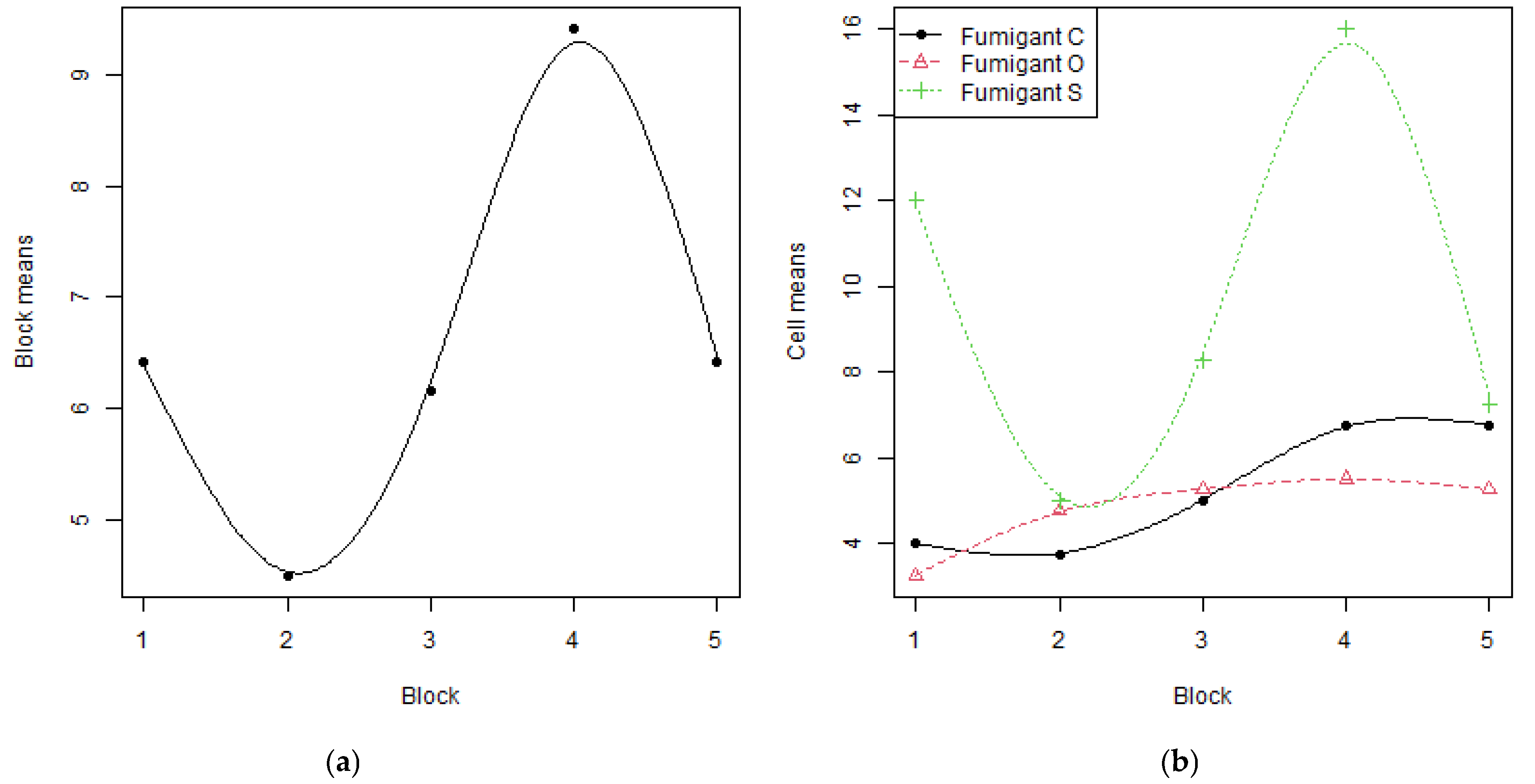
Figure 2.
Plots of (a) block means and (b) cell means versus blocks.
The fumigant F contrast of degree one has a p-value of 0.0000 (0.0019), and that of degree two has a p-value of 0.0023 (0.0000). The strong fumigant effect is due to a very strong quadratic effect and also features a strong linear effect. The plot of fumigant means versus fumigants in Figure 1a shows both the linear and quadratic effects. The plot in Figure 1b is the usual interaction plot of fumigant means for each block versus fumigants. Clearly, the (a) plot is an average over blocks of the (b) plots. The cell mean plot addresses the question: “as we pass through the levels of blocks, from block 1 to block 5, does the relationship between the cell means and fumigants change?” Subjectively, it would seem that it does for blocks 1 and 4.
The block F contrast p-values are 0.0810 (0.0809), 0.8588 (0.8604), 0.0009 (0.0007) and 0.4277 (0.4312). The very strong block effect is due principally to the cubic effect. The weak linear effect is perhaps an alias of the cubic effect. The plot of block means versus blocks in Figure 2a clearly shows the strong cubic effect. The plot in Figure 2b is the usual interaction plot of block means for each fumigant versus blocks. Clearly, the (a) plot is an average over fumigants of the (b) plots. The cell mean plot addresses the question: “as we pass through the levels of fumigants, from fumigant C to S and then to O, does the relationship between the cell means and blocks change?” Subjectively, it would seem that the relationship for the fumigant S is quite different from the other relationships. The former is strongly cubic, whereas for the other fumigants, it is approximately linear.
The ordered F interaction contrast p-values are 0.3051 (0.3060), 1.0000 (0.9912), 0.0011 (0.0011) and 0.4370 (0.4378), corresponding to degree one in fumigants and 0.9661 (0.9692), 0.4956 (0.4982), 0.0110 (0.0104) and 0.6414 (0.6411), corresponding to degree two in fumigants. The significant interaction effect is due principally to the effects of degree (1, 3) and (2, 3). In terms of generalised correlations, the (1, 3) effect suggests that as the fumigants increase linearly, that is, from fumigant C to S and then O, over the three-dimensional surface, there is a cubic effect. The (2, 3) effect is harder to interpret directly.
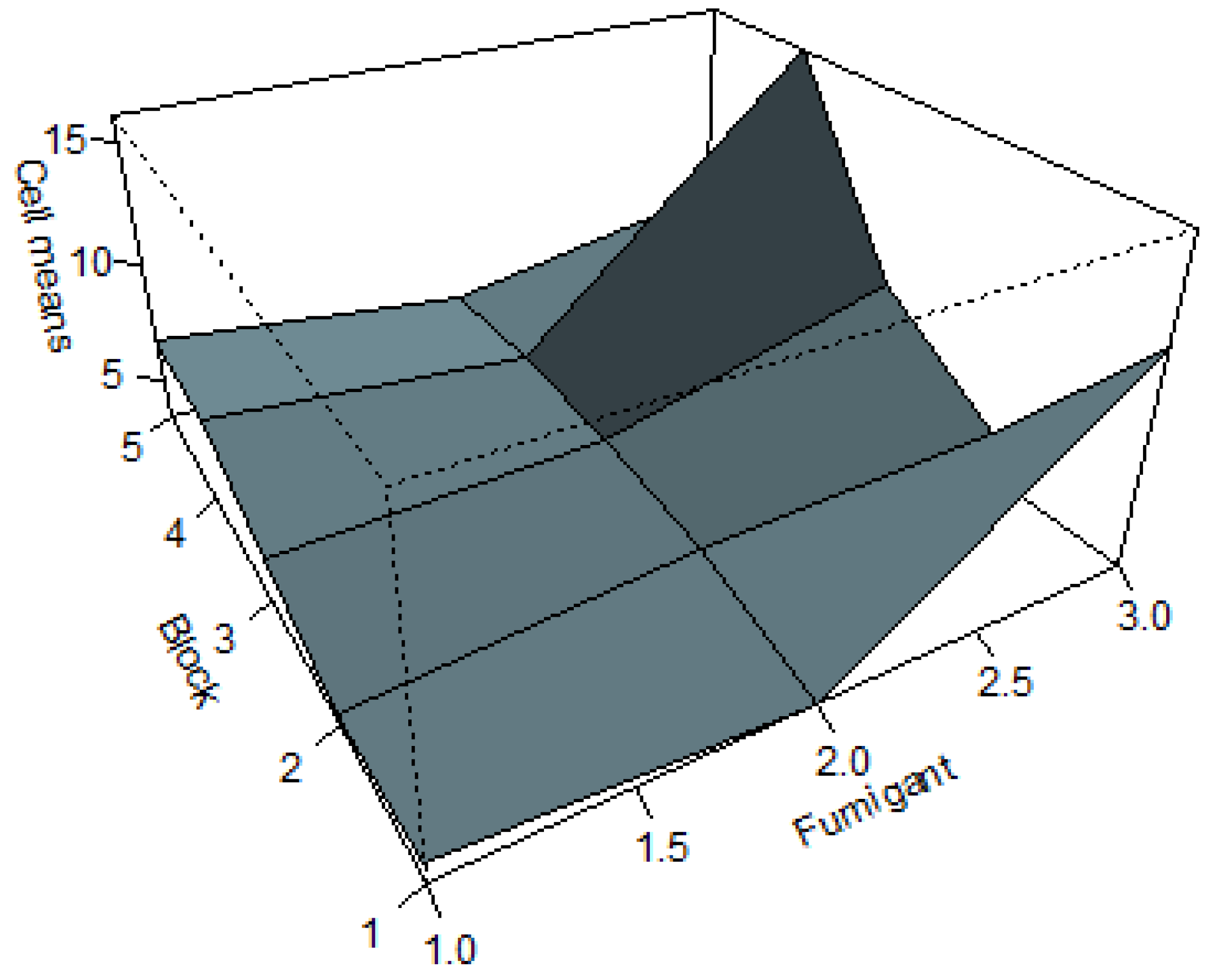
Figure 3 gives the three-dimensional plot of cell mean responses against the levels of both fumigants and blocks. The interaction plots are apparent as slices of this plot. Though the main effects plot shows a quadratic shape on average, the (1, 3) effect suggests that over the entire three-dimensional surface, the effect is more complex than that.
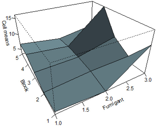
Figure 3.
The number of wireworms plotted against the levels of both factors.
Lizard data. The data in Table 2 come from Manly ([14] p. 144) and relate to the number of ants consumed by two sizes of eastern horned lizards over a four-month period. As lizard size has only two levels, it could be considered as either an ordered or unordered variable. The analysis here assumes the former. Natural scores 1, 2, 3, 4 for months are used as are 1, 2 for lizard size. These data were analysed in Rayner and Livingston, Jr. ([14], Section 6.3) using generalised correlations.
Table 2.
Ants consumed by lizards of two sizes over four months.
The following p-values are based on F sampling distributions with permutation test p-values based on 1,000,000 permutations in parentheses. As in the previous example, there is good agreement between the F and permutation test p-values. R output for the ANOVA follows.
| Analysis of Variance Table | |||||
| Response: response | |||||
| Df | Sum Sq | Mean Sq | F value | Pr (>F) | |
| month | 3 | 1,379,495 | 459,832 | 14.062 | 9.49 × 10⁻⁵ *** |
| size | 1 | 146,172 | 146,172 | 4.150 | 0.0505 |
| month:size | 3 | 294,009 | 98,003 | 4.470 | 0.0617 |
| Residuals | 16 | 523,222 | 32,701 | 2.997 | |
A standard replicated two-factor ANOVA had a lizard size p-value of 0.0505 (0.0450), a month p-value of 0.0001 (0.0001) and an interaction p-value of 0.0617 (0.0511). The Shapiro–Wilk test for normality of the residuals had a p-value of 0.0860. By ‘eyeballing’ the data, it would appear that larger lizards tend to eat more than smaller lizards. Since the p-values of the two lizard sizes straddle 0.05, this effect is borderline significant at the 0.05 level. Months are significant at the 0.001 level.
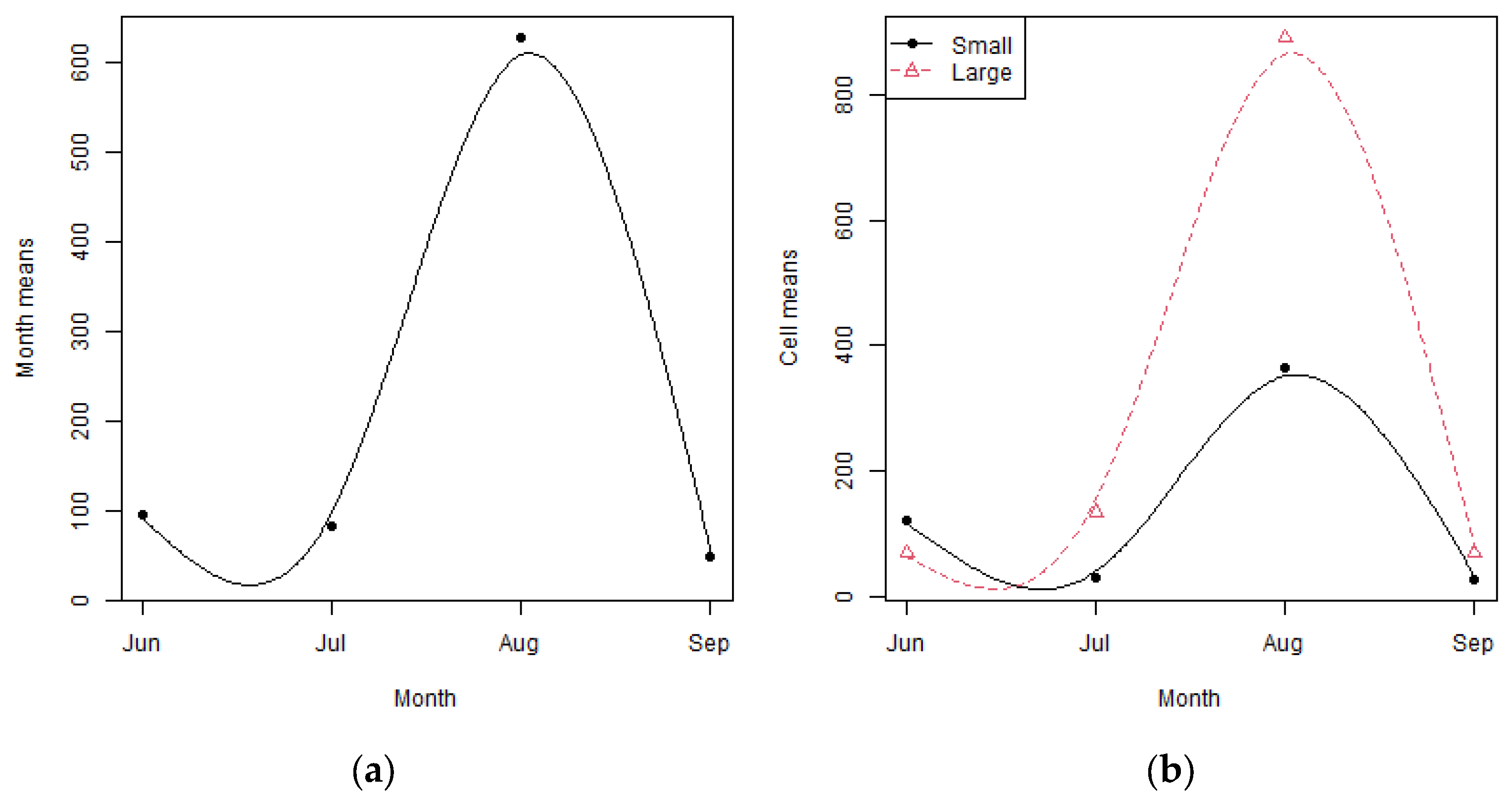
Figure 4 and Figure 5 give the standard plots. From Figure 4a, as we pass from June to September, the number of ants consumed decreases, increases and then decreases. The standard interaction plot in Figure 4b shows a similar but different relationship of ants consumed versus the month for both small and large lizards. Figure 4a is clearly an average of the plots for large and small lizards.
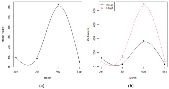
Figure 4.
Plots of (a) mean ants consumed and (b) cell means versus month.
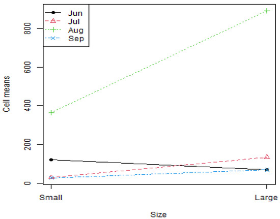
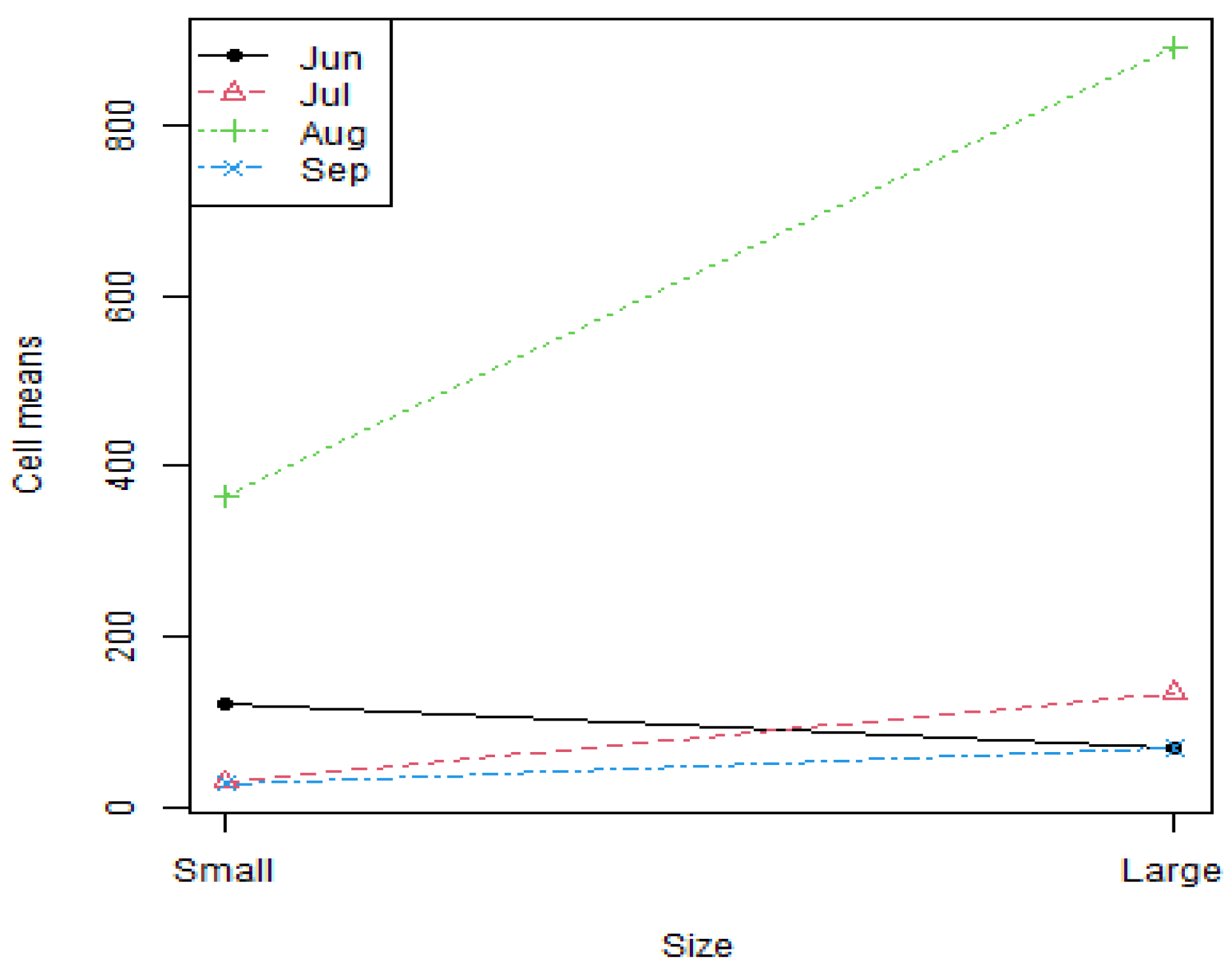
Figure 5.
Plots of mean ants consumed versus lizard size.
We do not give the trivial lizard size main effect plot that simply plots (large, 145.8333) and (small, 67.5417). Figure 5 is the standard interaction plot of month cell means against lizard size. Clearly, the August effect is different from that for the other months. It is also apparent in Figure 5 that the means for large and small lizards are different, as are the variances.
The orthonormal F contrast month p-values of degree one to three are 0.2371 (0.2427), 0.0015 (0.0007) and 0.0001 (0.0001), respectively. There are strong quadratic and cubic effects.
There are no lizard size contrasts, as there are only two levels of the factor lizard size.
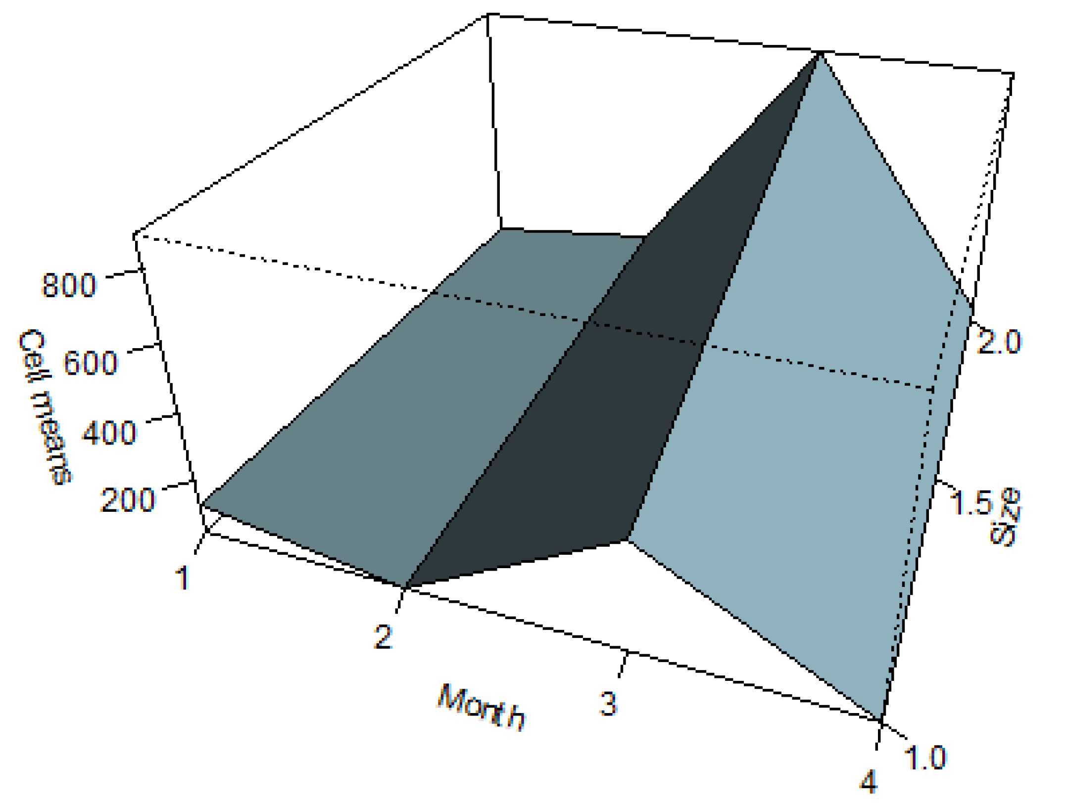
Although the interaction is not significant at the 0.05 level (p-value 0.0617), its ordered contrasts are interesting. The degree (1, 1), (1, 2) and (1, 3) orthonormal contrasts have p-values of 0.3077 (0.3163), 0.0452 (0.0391) and 0.0945 (0.0914), respectively. The degree (1, 2) effect objectively indicates that over the whole table, as we pass from small to large lizards, there is a predominantly quadratic effect in the number of ants consumed. In Figure 6, this is indicated by the ‘wrinkle’ corresponding with August. Also, as is apparent in the cell mean plots, patterns of ants consumed over months, although cubic but predominantly quadratic for both, are different in large and small lizards.
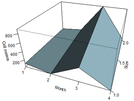
Figure 6.
The number of lizards consumed against the levels of both factors.
The Rayner and Livingston, Jr. [12] analysis allows the response to have second- and third-degree effects, but here, we are only interested in first-degree response effects. They report month permutation test p-values of 0.015 for degree two and 0.005 for degree three. These are consistent with the results reported here.
6. Conclusions
Contrasts have long been an essential tool for data analysts, and they feature in many undergraduate courses. However, the usual focus is on factors with unordered levels and balanced designs in which all the factor levels have the same number of observations. Here, our primary foci have been on main-effects factors for which the levels of the factor are ordered as well as on the interaction between two factors for which the levels of both factors are ordered.
As for the example in Snedecor and Cochran (1989, see [3], Section 12.8), the usual approach for a single factor with unordered levels is to decompose the treatment sum of squares and form ratios having the F1,edf distribution. The underlying theory is omitted. The treatment in Section 2 allows for factors with both unordered and ordered levels and gives the underlying theory.
The treatment in Section 3 is essentially for the two-factor fixed-effects ANOVA and gives the appropriate theory for interaction contrasts for factors having levels that are either unordered or ordered. Then, Section 4 focuses on the case when the levels for both factors are ordered and the contrasts may be interpreted as generalised correlations.
Previously, many data analysts drew subjective conclusions based on factor mean plots and cell mean plots. The use of contrasts allows for deeper, objective conclusions to be drawn.
Author Contributions
Conceptualization, J.C.W.R.; methodology, J.C.W.R. and G.C.L.J.; software, G.C.L.J.; validation, J.C.W.R. and G.C.L.J.; formal analysis, J.C.W.R. and G.C.L.J.; investigation, J.C.W.R. and G.C.L.J.; resources, J.C.W.R. and G.C.L.J.; data curation, G.C.L.J.; writing—original draft preparation, J.C.W.R.; writing—review and editing, J.C.W.R. and G.C.L.J.; visualization, J.C.W.R. and G.C.L.J.; supervision, J.C.W.R.; project administration, J.C.W.R. All authors have read and agreed to the published version of the manuscript.
Funding
This research received no external funding.
Institutional Review Board Statement
Not applicable.
Informed Consent Statement
Not applicable.
Data Availability Statement
Not applicable.
Conflicts of Interest
The authors declare no conflict of interest.
References
- Box, G.E.; Hunter, W.G.; Hunter, J.S. Statistics for Experimenters: Design, Innovation, and Discovery, 2nd ed.; Wiley: New York, NY, USA, 2005. [Google Scholar]
- Draper, N.R.; Smith, H. Applied Regression Analysis, 3rd ed.; Wiley: New York, NY, USA, 1998. [Google Scholar] [CrossRef]
- Snedecor, G.W.; Cochran, W.G. Statistical Methods, 8th ed.; Iowa State University Press: Ames, IA, USA, 1989. [Google Scholar]
- Kuehl, R. Design of Experiments: Statistical Principals of Research Design and Analysis; Duxbury Press: Belmont, CA, USA, 2000. [Google Scholar]
- Thas, O.; Best, D.J.; Rayner, J.C.W. Using orthogonal trend contrasts for testing ranked data with ordered alternatives. Stat. Neerl. 2012, 66, 452–471. [Google Scholar] [CrossRef]
- Rayner, J.C.W.; Livingston, G.C., Jr. Orthogonal contrasts for both balanced and unbalanced designs and both ordered and unordered treatments. Stat. Neerl. 2023. [Google Scholar] [CrossRef]
- Rayner, J.C.W.; Beh, E.J. Towards a better understanding of correlation. Stat. Neerl. 2009, 63, 324–333. [Google Scholar] [CrossRef]
- Rayner, J.C.W.; Thas, O.; De Boeck, B. A generalised Emerson recurrence relation. Aust. N. Z. J. Stat. 2008, 50, 235–240. [Google Scholar] [CrossRef]
- Craig, A.T. Note on the Independence of Certain Quadratic Forms. Ann. Math. Stat. 1943, 14, 195–197. [Google Scholar] [CrossRef]
- Lancaster, H.O. The Helmert matrices. Am. Math. Mon. 1965, 72, 4–12. [Google Scholar] [CrossRef]
- Rayner, J.; Best, D. A Contingency Table Approach to Nonparametric Testing; Chapman & Hall: Boca Raton, FL, USA; CRC: Boca Raton, FL, USA, 2001. [Google Scholar]
- Rayner, J.C.W.; Livingston, G.C., Jr. An Introduction to Cochran–Mantel–Haenszel Testing and Nonparametric ANOVA; Wiley: Chichester, UK, 2023. [Google Scholar]
- Ladell, W.R.S.; Cochran, W.G. Field experiments on the control of wireworms. Ann. Appl. Biol. 1938, 25, 341–382. [Google Scholar] [CrossRef]
- Manly, B.F.J. Randomization, Bootstrap, and Monte Carlo Methods in Biology, 3rd ed.; Chapman & Hall: London, UK, 2007. [Google Scholar]
Disclaimer/Publisher’s Note: The statements, opinions and data contained in all publications are solely those of the individual author(s) and contributor(s) and not of MDPI and/or the editor(s). MDPI and/or the editor(s) disclaim responsibility for any injury to people or property resulting from any ideas, methods, instructions or products referred to in the content. |
© 2023 by the authors. Licensee MDPI, Basel, Switzerland. This article is an open access article distributed under the terms and conditions of the Creative Commons Attribution (CC BY) license (https://creativecommons.org/licenses/by/4.0/).