Abstract
This paper presents an advanced hierarchical classification framework using the Random Forest (RF) algorithm to segment and classify large-scale point clouds of heritage buildings. By integrating the Uniclass classification system into a multi-resolution workflow, the research addresses key challenges in point cloud classification, including class imbalance, computational constraints, and semantic overlap at coarse resolutions. It adopts an experimental research design using the heritage case study from Royal Greenwich Museum in the UK. The findings demonstrate that industry classification systems and data taxonomies can be aligned with machine learning workflows. This study contributes to Heritage-Building Information Modelling (HBIM) by proposing optimised hierarchical structures and scalable machine learning techniques. The research concludes with recommendations for future research, based on the performance of the Random Forest technique, particularly in further developing AI applications within HBIM.
1. Introduction
This study examines the application of hierarchical classification techniques for the semantic segmentation of large-scale point cloud datasets derived from cultural heritage buildings, with a particular emphasis on aligning classification outputs to the UK’s Uniclass taxonomy. Hierarchical classification, a machine learning paradigm in which class labels are structured in a parent–child hierarchy, facilitates the progressive refinement of predictions from broader to more specific semantic categories. Unlike flat classification models, hierarchical approaches leverage inter-class relationships to improve both predictive accuracy and computational scalability—capabilities especially pertinent in Heritage Building Information Modelling (HBIM), where datasets are characteristically multi-scale, noisy, and subject to significant class imbalance [1].
This methodological approach is particularly well suited to HBIM workflows, wherein architectural complexity and data heterogeneity pose substantial barriers to automation. By accommodating varying levels of semantic granularity and spatial resolution, hierarchical classification enables more precise, context-aware segmentation of intricate heritage geometries. Moreover, its potential for computational efficiency makes it a promising candidate for the scalable processing of high-density point clouds.
The research builds upon foundational work by Grilli et al. [2], Teruggi et al. [3], and Zhang et al. [4], each of whom explored multi-resolution classification strategies for built heritage datasets. However, these prior studies frequently employ bespoke or project-specific taxonomies, thereby limiting their alignment with formalised information management frameworks. This study addresses this limitation by embedding the NBS Uniclass Element/Function (EF) table—a widely adopted classification schema in the UK construction sector—into a Random Forest-based hierarchical segmentation pipeline.
Uniclass forms part of the National Building Specification (NBS), a UK-developed digital framework designed to standardise information across the built environment lifecycle. It organises construction-related data into a coherent hierarchy encompassing buildings, systems, elements, and products, thereby enabling consistent categorisation and seamless integration with Building-Information Modelling (BIM) processes. Its interoperability across disciplinary boundaries and conformance with international standards, including ISO 19650 [5,6], make it a particularly suitable candidate for classification-driven HBIM methodologies.
The principal contributions of this research are fourfold: (1) the development of a Uniclass-aligned hierarchical classification framework tailored for HBIM datasets; (2) the implementation of a novel workflow for point cloud labelling using CloudCompare; (3) an evaluation of classification accuracy across multiple semantic levels and spatial resolutions; and (4) a critical assessment of challenges inherent in large-scale segmentation, including class imbalance, geometric ambiguity, and resolution sensitivity. In doing so, this study not only advances current HBIM segmentation practices but also enhances the integration of UK classification standards into machine learning-based heritage documentation workflows.
Related Work and State-of-the-Art Methods
Machine learning (ML) techniques have become increasingly integral to Historic-Building Information Modelling (HBIM), offering scalable and efficient solutions for tasks including point cloud classification, semantic enrichment, and the semi-automated generation of geometry from spatial data. Among classical approaches, Decision Trees and Random Forests (RFs) remain particularly prevalent due to their robustness to noise, interpretability, and compatibility with handcrafted features—attributes of significant importance in heritage contexts, where data variability and limited annotated ground truth are commonplace [7,8].
RF classifiers have been effectively deployed in various heritage applications, including façade element recognition [9], masonry damage mapping [10], and hierarchical semantic segmentation of architectural features such as vaults, arches, and cornices [3,11]. These contributions collectively established the methodological foundations for hierarchical classification in HBIM. However, a notable limitation in this body of work is the widespread use of ad hoc or domain-specific taxonomies, which limits interoperability with standardised information management systems.
Building on these classical approaches, subsequent research has integrated RF classification outputs with rule-based geometry generation, often leveraging visual programming environments, such as Rhino and Grasshopper. For instance, Croce et al. [12] implemented a semi-automated Scan-to-HBIM pipeline, reporting classification precision rates up to 93.49% across multiple case studies of historic buildings. Parallel efforts by Wang et al. [13] sought to improve spatial label coherence through the incorporation of Markov Random Fields (MRFs), although these methods introduced additional computational overheads.
In recent years, deep learning (DL) has emerged as a transformative force in 3D semantic segmentation. Architectures such as PointNet [14], graph convolutional networks, and multimodal neural models enable direct learning from unstructured data formats, circumventing the need for handcrafted feature engineering. Within the cultural heritage domain, Belhi et al. [15] developed a multitask hierarchical classifier that fused visual and textual features, improving annotation performance on under-labelled datasets through multimodal learning. Similarly, Condorelli et al. [16] employed neural networks to detect lost architectural elements in historical film archives, thereby supporting the photogrammetric reconstruction of inaccessible or deteriorated assets.
Nonetheless, DL methodologies face several persistent challenges in HBIM applications, notably the scarcity of annotated heritage datasets, substantial computational requirements, and limited alignment with formal classification standards such as Uniclass. In this context, hybrid approaches—combining classical ML algorithms with rule-based inference mechanisms and ontology-driven frameworks—offer a pragmatic compromise, balancing scalability, domain adaptability, and semantic rigour.
2. Material and Methods
This study adopts an experimental methodology to evaluate the integration of a Random Forest (RF) machine learning model with the Uniclass classification system for hierarchical semantic segmentation of cultural heritage point cloud data. The methodology encompasses four key phases: (1) review of existing ontological frameworks; (2) critical appraisal and refinement of the Uniclass Element/Function (EF) table for applicability to heritage datasets; (3) dataset preparation for hierarchical classification; and (4) implementation and evaluation of the classification pipeline. The subsequent subsections detail the experimental setup, ontological decisions, and classifier architecture.
2.1. Experimental Setup
The hierarchical classification pipeline was developed using Python 3.11.2 primarily leveraging the scikit-learn 0.23.2 library for core machine learning functionality and enhanced through GPU-accelerated modules from the cuML RAPIDS suite to expedite computationally intensive tasks. GPU support was particularly beneficial during the training of RF classifiers, dimensionality reduction, and dataset resampling processes.
To manage the large-scale point cloud dataset, out-of-core processing was employed using Polars, Open3D, and PyntCloud. CloudCompare was utilised for visual inspection and qualitative validation of classification outputs.
All experiments were conducted on a mid-to-high-performance desktop workstation equipped with an AMD Ryzen 5 3600 CPU, 32 GB DDR4 RAM, and an NVIDIA RTX 4090 GPU. While this hardware configuration lies between standard laboratory computing and high-performance computing (HPC) environments, the sheer volume and granularity of the dataset imposed computational constraints. These limitations necessitated the adoption of a multi-resolution, hierarchical classification strategy to ensure computational feasibility and model scalability.
2.2. Ontological Reuse and Uniclass Review
The reuse of existing ontologies within the built environment domain offers significant foundational benefits for the development of novel semantic classification frameworks. As argued by Tibaut and Guerra De Oliveira [17], ontological reuse enhances semantic consistency, promotes interoperability, and reduces the complexity associated with schema design. In line with these principles, the Uniclass Element/Function (EF) table was selected as the primary classification ontology for semantic labelling of the heritage point cloud dataset used in this study.
A structured review of relevant Uniclass EF codes was conducted across three semantic tiers—Tier 1 (broad functional categories), Tier 2 (intermediate architectural components), and Tier 3 (specific sub-elements). Although the full Uniclass EF taxonomy encompasses a comprehensive range of built environment assets, the classification scope was refined to suit the characteristics of the case study building. In total, 13 of the original 15 Tier 1 classes, 23 of 68 Tier 2 classes, and 21 of 114 Tier 3 classes were identified as relevant for inclusion. Additionally, a custom class, designated EF_XX, was introduced to capture scanning artefacts such as noise, reflective anomalies, and the presence of human silhouettes. All selected Tier 2 and Tier 3 categories were explicitly defined ontologically to ensure semantic clarity during both model training and classification phases.
The decision to adopt the Uniclass EF schema as the primary classification framework was informed by its demonstrable suitability for HBIM and machine learning-based applications. Comparative experimentation confirmed that Uniclass offers several advantages over alternative classification systems such as IFC, CCI, or ETIM. These competing taxonomies often employ broad or inconsistently structured category groupings, limiting their effectiveness in hierarchical modelling of complex heritage assets.
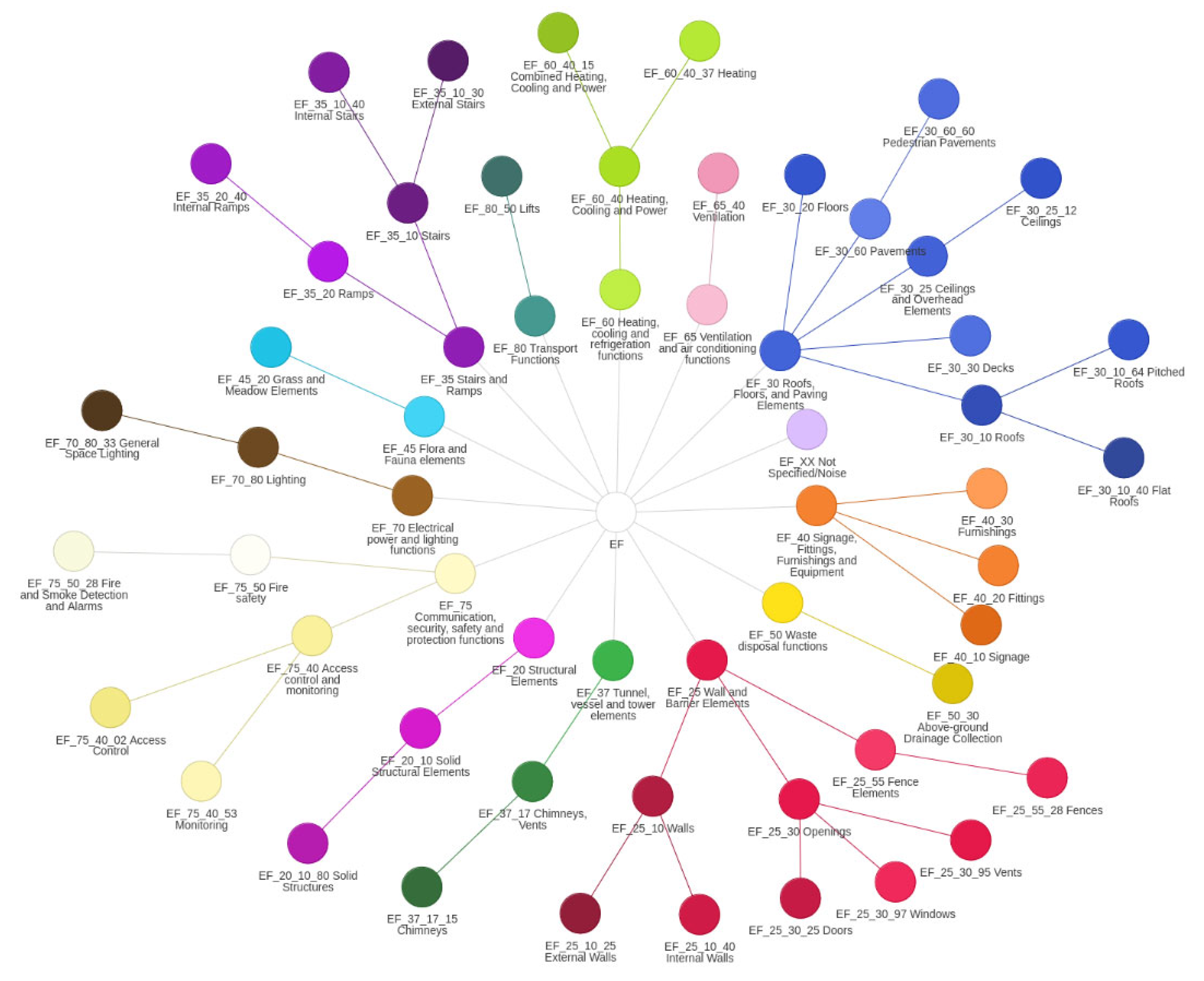
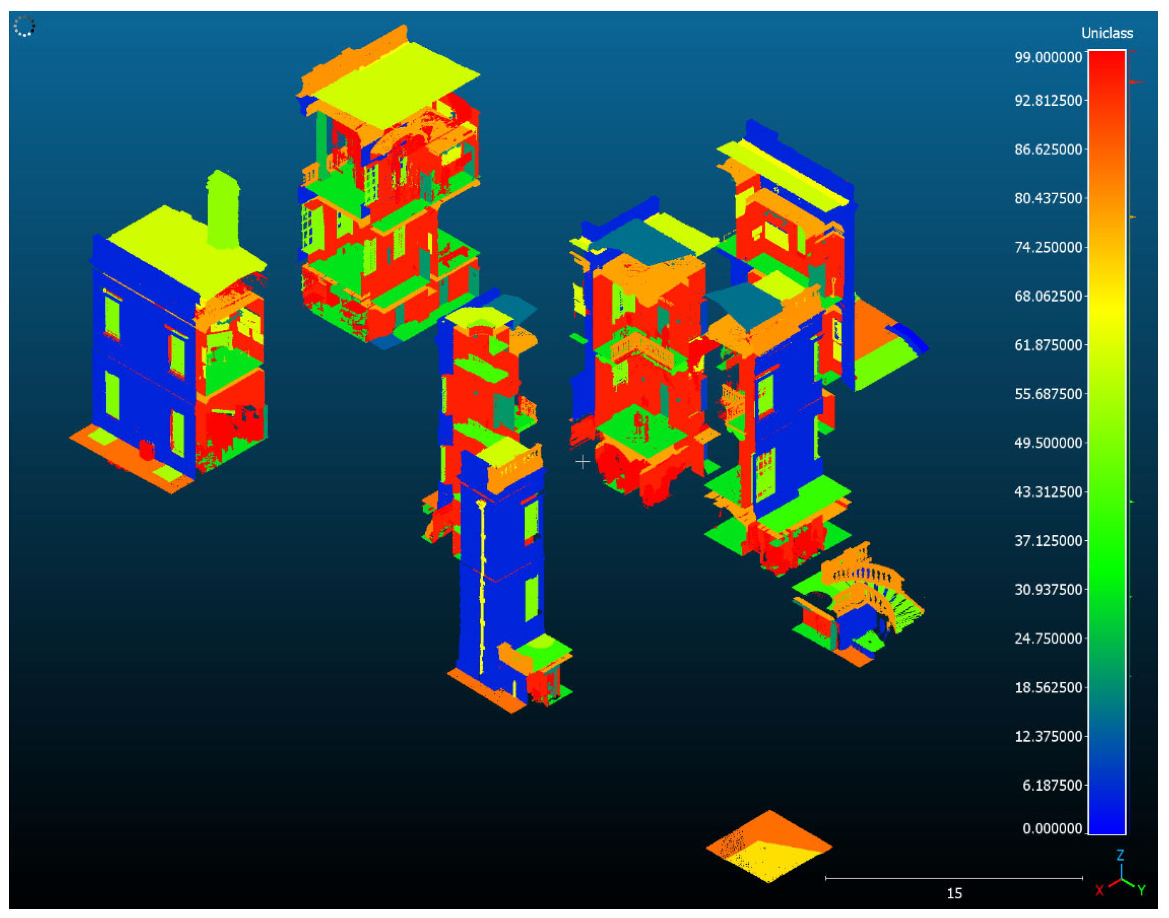
In contrast, Uniclass provides a well-defined, multi-level taxonomy specifically aligned with UK construction practices and compliant with ISO 19650 information management principles [18]. Its modular architecture allows for consistent labelling of both coarse and fine-grained building components. This flexibility is essential for the development of classification models capable of addressing the scale, diversity, and detail inherent in large heritage point cloud datasets. Figure 1 shows the Uniclass classification system for heritage dataset structuring at Level 1, Level 2 and Level 3 hierarchical categories.

Figure 1.
Uniclass classification dendrogram.
2.3. Dataset Case Study Building
The Queen’s House, designed by Inigo Jones and completed in 1662, is widely regarded as a seminal work in the history of British architecture. Originally commissioned by Anne of Denmark and later completed under the patronage of Queen Henrietta Maria, the building was conceived as both a royal residence and a hunting lodge [19]. Its design marked the first systematic application of Palladian principles—symmetry, classical orders, and mathematical proportion—within English architecture, reflecting Jones’s exposure to Renaissance ideals during his formative studies in Italy.
Subsequently integrated into the architectural landscape of the Royal Hospital for Seamen at Greenwich, the Queen’s House forms part of a historically and architecturally significant ensemble of national importance [20]. Over the centuries, the building has undergone multiple phases of conservation, renovation, and adaptive reuse. It now functions as a central component of the National Maritime Museum, hosting a prominent fine art collection and serving as a venue for cultural and ceremonial events.
The enduring significance of the Queen’s House lies not only in its architectural innovation but also in its continuing contribution to the narrative of British design heritage, museology, and cultural identity [21]. Its blend of historical depth and contemporary relevance renders it an ideal subject for HBIM experimentation, particularly within the context of AI-enabled semantic segmentation and ontological classification.
2.4. Dataset Description and Subsampling
A high-resolution terrestrial laser-scanning (TLS) dataset comprising approximately 1.28 billion points was acquired from the Queen’s House case study and processed using a hierarchical semantic classification workflow. To enable scalable computation and multi-resolution learning, as shown in Table 1, the dataset was spatially subsampled into three distinct resolution levels: 50 mm (Level 1), 20 mm (Level 2), and 5 mm (Level 3). Independent Random Forest (RF) classifiers were trained at each level to progressively refine classification granularity while balancing computational demand.

Table 1.
Number of points achieved post-sub-sampling.
The Uniclass Element/Function (EF) taxonomy was adapted at each resolution level to reflect the geometric complexity and semantic richness attainable at the corresponding scale. This hierarchical segmentation strategy enabled semantic differentiation across coarse, intermediate, and fine-grained architectural features.
Seventeen geometric and radiometric features, including curvature, planarity, verticality, and RGB values, were computed for each point across all levels. The feature extraction methodology was designed to preserve geometric fidelity while reducing computational load, following best practices outlined by Ch, Jung, and Olsen [22].
2.5. Random Forest Configuration
The Random Forest (RF) model was configured to balance classification accuracy with computational efficiency, considering the extensive size of the heritage point cloud dataset as tabulated in Table 2.
Table 2.
Random Forest hyperparameters.
The classifier was composed of 200 decision trees, employing entropy as the splitting criterion to maximise information gain during feature partitioning. To prevent overfitting and ensure generalisability, a maximum tree depth of 8 was imposed, with a minimum of six samples per leaf and twelve samples required for internal node splitting. Model robustness was evaluated using a five-fold cross-validation strategy.
Although comprehensive hyperparameter optimisation was beyond the scope of this study, due to the computational demands associated with processing high-density point cloud data, the selected configuration was informed by best practices in heritage segmentation and machine learning literature. These settings offered a pragmatic trade-off, enabling effective learning from hierarchical features while maintaining tractable training times across the three resolution levels.
2.6. Training and Evaluation Approach
This study investigated two strategies for training and evaluating hierarchical Random Forest (RF) classifiers, each aligned with the semantic tiers of the adopted classification schema. While both approaches follow a multi-stage structure corresponding to the hierarchy of labels, they diverge in the mechanism by which class labels are transferred between successive levels. These strategies are derived from pre-existing methods in the literature and are used as best practice among studies across various sectors [23].
- Ground Truth Routing (proposed evaluation method): The first strategy, termed Ground Truth Routing, involves training and evaluating each classification level using the actual class labels from the manually annotated dataset. For instance, at Tier 3, only those points that are known (based on ground truth) to belong to the class Wall at Tier 2 are used to train a classifier that differentiates between Inner Wall and Outer Wall. This approach effectively isolates each hierarchical stage, enabling the performance of the classifier to be assessed without the confounding influence of upstream prediction errors. While this method presumes the availability of finely annotated data, rendering it less applicable in fully automated, real-world inference tasks, it offers a high-resolution diagnostic perspective. Specifically, it permits an objective evaluation of the intrinsic complexity of each classification step and the model’s discriminative power at varying semantic levels.
- Predicted Label Routing (alternative evaluation method): The second strategy, Predicted Label Routing, emulates operational HBIM scenarios wherein the outputs of higher-tier classifiers are used as inputs for subsequent levels. For example, any point predicted as Wall at Tier 2 is passed to the Tier 3 classifier, which attempts to further classify it as either Inner Wall or Outer Wall. This approach reflects a more realistic deployment scenario but introduces cumulative error propagation, whereby misclassifications at earlier stages negatively influence downstream performance. Additionally, due to potential discrepancies in dataset distribution across classification levels, auxiliary mechanisms, such as k-nearest neighbour (k-NN) label propagation, are required to maintain label continuity throughout the hierarchy.
To ensure a controlled and diagnostic evaluation of classification performance, this study adopted the Ground Truth Routing strategy. By intentionally decoupling hierarchical dependencies, the approach facilitates clearer attribution of model errors and performance limitations to specific semantic levels. Consequently, it provides a robust experimental foundation for understanding the capabilities and constraints of hierarchical RF classifiers in the context of semantic segmentation of heritage-building point clouds.
2.7. Research Process Implementation Plan
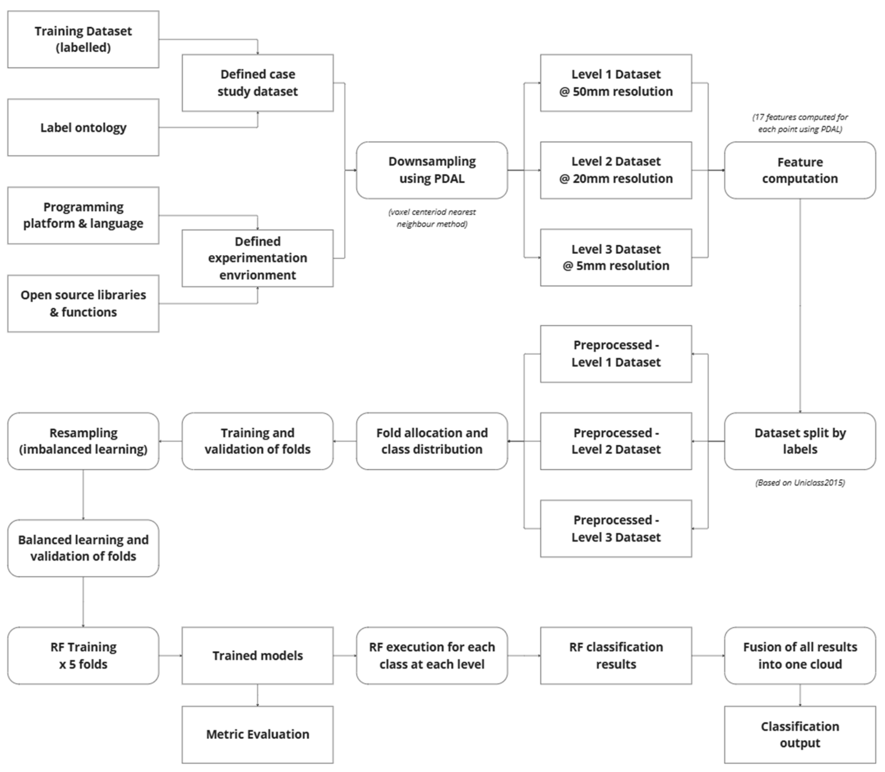
To effectively manage the scale, complexity, and semantic richness of the heritage-building point cloud dataset, a structured implementation workflow was developed and applied. The primary objective of this workflow was to facilitate a hierarchical classification process using Random Forest (RF) models while addressing challenges such as data volume, class imbalance, and semantic granularity. The overall process summarised in Figure 2, consists of three core stages: data preparation, model training and evaluation, and classification output synthesis.

Figure 2.
Random Forest implementation process workflow.
In the first stage, the raw labelled dataset was defined and structured based on a Uniclass-compliant ontology tailored to heritage-building typologies. The dataset was then spatially downsampled at three resolution levels—50 mm, 20 mm, and 5 mm—corresponding to the semantic depth required at Levels 1, 2, and 3 of the classification hierarchy. Feature descriptors were computed for each point using neighbourhood-based geometric analysis, providing the inputs required for machine learning. The data were further split by class labels and preprocessed to support balanced learning and stratified validation.
The second stage involved the construction and training of Random Forest classifiers using a five-fold cross-validation strategy. A combination of oversampling and editing techniques was employed to mitigate class imbalance, ensuring robust model generalisation. Classifiers were trained independently for each semantic level, and their outputs were evaluated using standard performance metrics. In the final stage, classification results from all levels were fused into a single coherent output, yielding a fully labelled point cloud aligned with the Uniclass Element/Function taxonomy. This workflow provided a scalable and repeatable methodology for heritage-specific HBIM segmentation, combining semantic precision with computational feasibility.
2.8. Random Forest Experiment Preparation
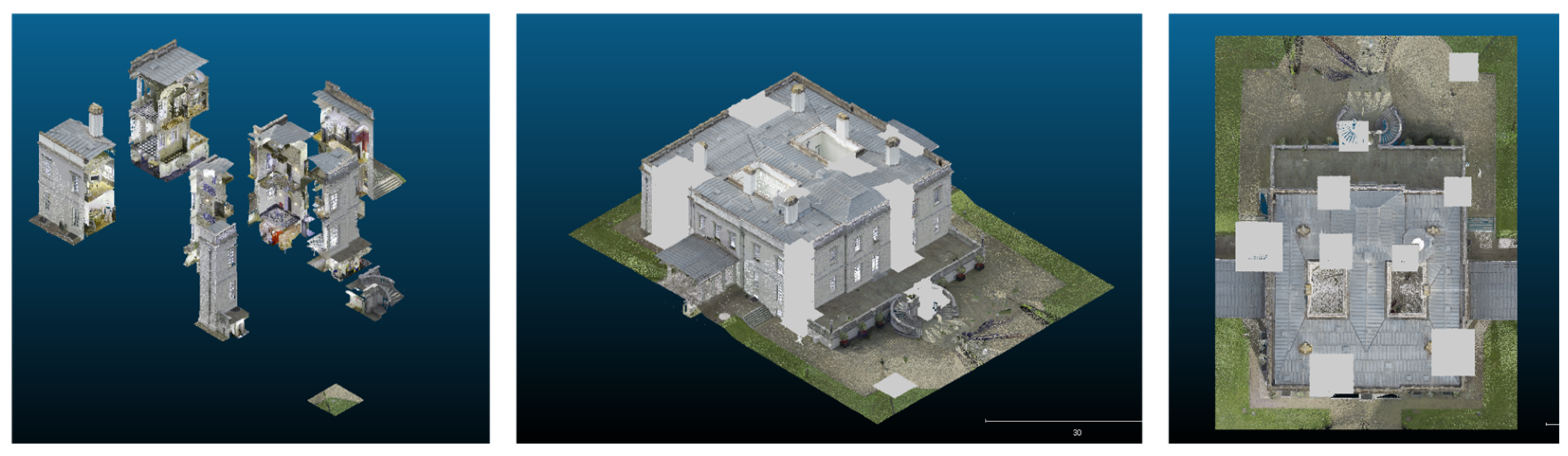
The experimental framework was applied to the full heritage building point cloud, comprising approximately 1.2 billion points. Given the substantial practical and computational constraints associated with annotating such a large-scale dataset, manual labelling was applied using slicing and scalar factor functions in CloudCompare software [24] to a strategically selected subset, equating to approximately 16% of the total dataset.
This subset, shown in grey in Figure 3, consisted of cuboidal volumes sampled from various spatial regions of the site. These volumes were manually annotated according to the Uniclass classification schema, broken down across three hierarchical levels (L1, L2, and L3). This process necessitated a detailed examination of the building’s physical components to determine which Uniclass categories were present within the dataset, and which were not.
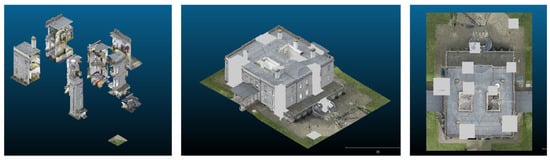
Figure 3.
Context of the selected training data shown in grey.
At Level 1, 14 broad element classes were identified, including categories such as EF_30 (Roof, Floors and Paving Elements) and EF_60 (Heating, Cooling, and Refrigeration Elements). At Level 2, this classification was refined into 23 subclasses, such as EF_30_20 (Floors), EF_30_60 (Pavements), and EF_60_40 (Heating, Cooling, and Power Appliances). At Level 3, the most detailed level, 21 subclasses were annotated, including elements such as EF_60_60 (Pedestrian Pavements) and EF_60_40_37 (Heating).
The selected 16% subset was designed to be both geometrically diverse and semantically rich, thereby providing a representative training corpus without imposing prohibitive manual labelling or computational burdens. The fully labelled dataset is illustrated in Figure 4 and was used for training the Random Forest classifiers.
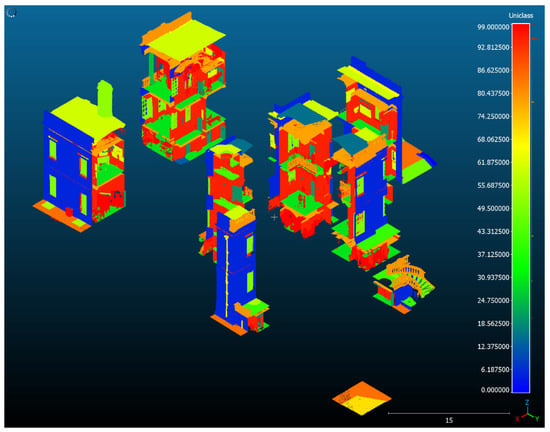
Figure 4.
Manually labelled training dataset.
Manual annotation was exclusively conducted at the most granular level (Level 3). The higher-level categories (Levels 1 and 2) were then programmatically derived by aggregating the Level 3 labels according to the Uniclass parent–child taxonomy. This top-down strategy significantly reduced annotation workload while allowing the classifier to be trained across a semantic hierarchy—capturing both general and specific building element features.
To manage the enormous dataset size, voxel-based subsampling was performed using the filters.voxelcentroidnearestneighbor function in PDAL, supported by custom Python scripts for data consistency across classification levels. The subsampling procedure discretised the 3D point cloud into voxel grids at progressively finer resolutions—50 mm for Level 1, 20 mm for Level 2, and 5 mm for Level 3. For each voxel, a single representative point was selected based on proximity to the voxel centroid, preserving spatial structure while substantially reducing dataset volume.
To support robust training and evaluation, the dataset was partitioned using an octree-based spatial heuristic that preserved contiguity and class balance across cross-validation folds. This spatially aware partitioning mitigated the risks of spatial autocorrelation and class imbalance, both of which can distort classifier performance metrics if unaddressed.
Each classifier was therefore trained on a manageable yet representative dataset, ensuring computational tractability while retaining critical spatial and semantic features. A five-fold cross-validation scheme was employed throughout, providing reliable performance estimates and minimising risks associated with overfitting.
2.8.1. Class Imbalance Challenge
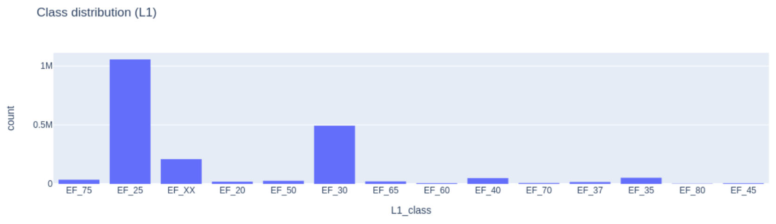
A specific challenge encountered in this experiment is pronounced class imbalance. In this study, an example of such imbalance emerges in the L1 taxonomy, where the minority class EF_75 (Communications, security, safety, and protection functions) has only about 2000 points, contrasted with the majority class EF_25 (Walls and barrier elements), which includes roughly 1.1 million points. Training a classifier on skewed data risks creating strong biases against underrepresented classes, leading to poor overall performance. Figure 5 shows the Level 1 class distribution reflecting the imbalance.
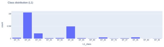
Figure 5.
Level 1 class distribution graph.
To mitigate this issue, resampling techniques were employed to rebalance the training-data distribution. Specifically, a hybrid sampling approach combining random under-sampling of majority classes and Synthetic Minority Over-sampling Technique (SMOTE) for minority classes was implemented. SMOTE generates synthetic examples by interpolating feature values within minority classes, while random under-sampling reduces redundant data points from dominant classes. This strategy effectively balanced the dataset and decreased the classifier’s bias against minority classes.
However, merely adjusting sample proportions does not fully resolve class imbalance, especially within spatial data. Spatial autocorrelation introduces complexities: adjacent points typically share labels, violating assumptions of sample independence inherent in conventional machine learning evaluations. Random partitioning of data can thus inadvertently inflate model performance estimates, undermining their reliability.
To address spatial dependence and ensure robust cross-validation, an octree-based heuristic approach was developed. The point cloud was partitioned into spatially coherent blocks using an octree structure, allowing for controlled allocation of these blocks to cross-validation folds. By evaluating class distributions within each octree node, folds could be balanced effectively, guaranteeing representation of each class while preserving spatial contiguity. This approach provided a rigorous and spatially informed evaluation framework, mitigating the influence of spatial autocorrelation and delivering more reliable performance metrics.
2.8.2. Additional Feature Computation
To effectively characterise and differentiate individual points within the dataset, a comprehensive set of 17 descriptive features was computed for each point. These features comprised both geometric descriptors and RGB colour values, collectively designed to capture local structural patterns and surface appearance.
Geometric features were derived using neighbourhood analysis functions in PDAL, based on the 10 to 12 nearest neighbours per point. This approach enabled the extraction of local shape descriptors, which characterise the structural and spatial configuration of the surrounding 3D geometry. The computed features are summarised in Table 3, with each descriptor representing a specific aspect of local geometric complexity, spatial distribution, or surface orientation.
Table 3.
Geometric features employed.
In addition to these 14 geometric attributes, the raw RGB colour intensities were included as features, resulting in a total of 17 dimensions per point. This multimodal feature set integrates both spatial morphology and visual appearance, which is particularly useful when classifying elements in architecturally diverse heritage environments.
3. Results
This section presents the outcomes of the hierarchical classification approach across both a preliminary pilot test on a small subset of the data and the subsequent full-scale experiments. Emphasis is placed on evaluating the methodology’s capacity to accurately segment and classify point clouds at multiple levels of spatial and semantic granularity, together with an assessment of computational feasibility and interpretability. The first subsection details the soft test outcomes, which served as a benchmark for estimating processing times and accuracy levels. Subsequent subsections elaborate on the results at each of the three classification levels (L1, L2, and L3) when applied to the entire case study dataset.
The results from the soft test, performed on a limited gallery room sample, were promising. For Level 1 (L1), the classification process took approximately 10.3 h to complete 800 iterations of training, yielding a balanced accuracy of 75.7% and a weighted F1 score of 92.2%. At Level 2 (L2), requiring around 7.9 h and involving 800 iterations, the balanced accuracy decreased slightly to 74.9%, while the weighted F1 score stood at 88.3%. For Level 3 (L3), performance was assessed over just five iterations, primarily because the higher spatial resolution demanded longer computational times (about 1.1 days of processing). Despite the reduced number of training cycles, the L3 classification still achieved a balanced accuracy of 74.1% and a weighted F1 score of 88.1%.
While these soft test results stem from a relatively small input dataset with fewer active classes, they do offer indicative insights into classification viability, computational cost, and the anticipated level of accuracy. These insights were considered satisfactory for proceeding with a full-scale experiment on the entire dataset, which is presented in the subsequent sections.
3.1. Full Dataset Level 1 Results
The first tier of classification (L1) entailed applying a single Random Forest model to the 50 mm subsampled cloud, assigning each point to one of 14 top-level Uniclass labels. In many respects, this constitutes the most challenging layer of the hierarchical approach. First, the classifier must distinguish amongst the greatest number of categories at any single level, which necessarily increases the scope for misclassification. Second, the 5 cm resolution cloud obscures the fine-grained geometric features that might otherwise help differentiate smaller or intricately detailed elements.
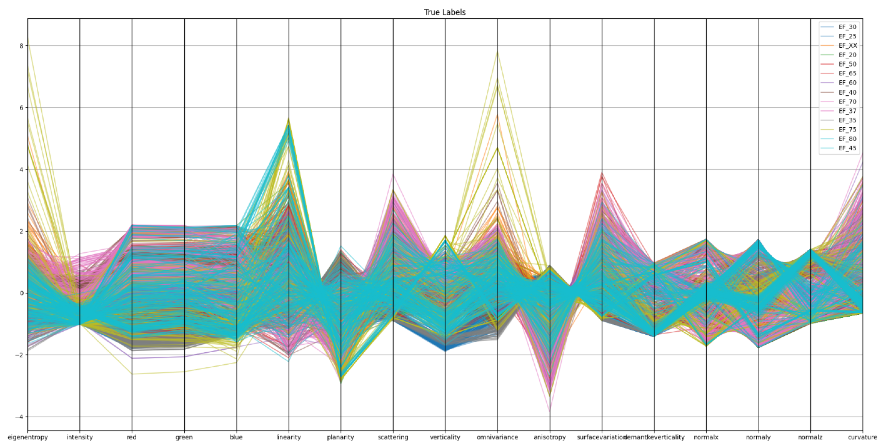
Figure 6 shows the parallel coordination plot for Level 1 classifiers. In Figure 6, each coloured line represents a single point in the 5 cm subsampled point cloud, coloured by its ground-truth L1 class. The plot shows normalised values across 17 geometric and radiometric features. The extensive overlap between classes indicates limited separability in feature space, suggesting that the input features are not sufficiently discriminative at this resolution, particularly for finer or minority classes.
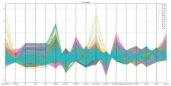
Figure 6.
Parallel coordinates plot for Level 1. Each coloured line represents a single point in the 5 cm subsampled point cloud, coloured by its ground-truth L1 class. The plot shows normalised values across 17 geometric and radiometric features. The extensive overlap between classes indicates limited separability in feature space, suggesting that the input features are not sufficiently discriminative at this resolution—particularly for finer or minority classes.
An initial inspection of the feature-space distribution confirms that numerous classes display substantial overlap across geometric descriptors, such as curvature, verticality, or planarity. Consequently, the chosen feature set does not clearly demarcate the class boundaries in low-resolution data.
Nevertheless, the classifier performed noticeably better on classes whose geometric properties remain relatively stable at this scale, including EF_30 (Roofs, floors, and paving elements) and EF_25 (Walls and barriers). Larger structural elements, by virtue of having extended planar or linear surfaces, appear to retain discriminative geometric signals even at coarser resolutions.
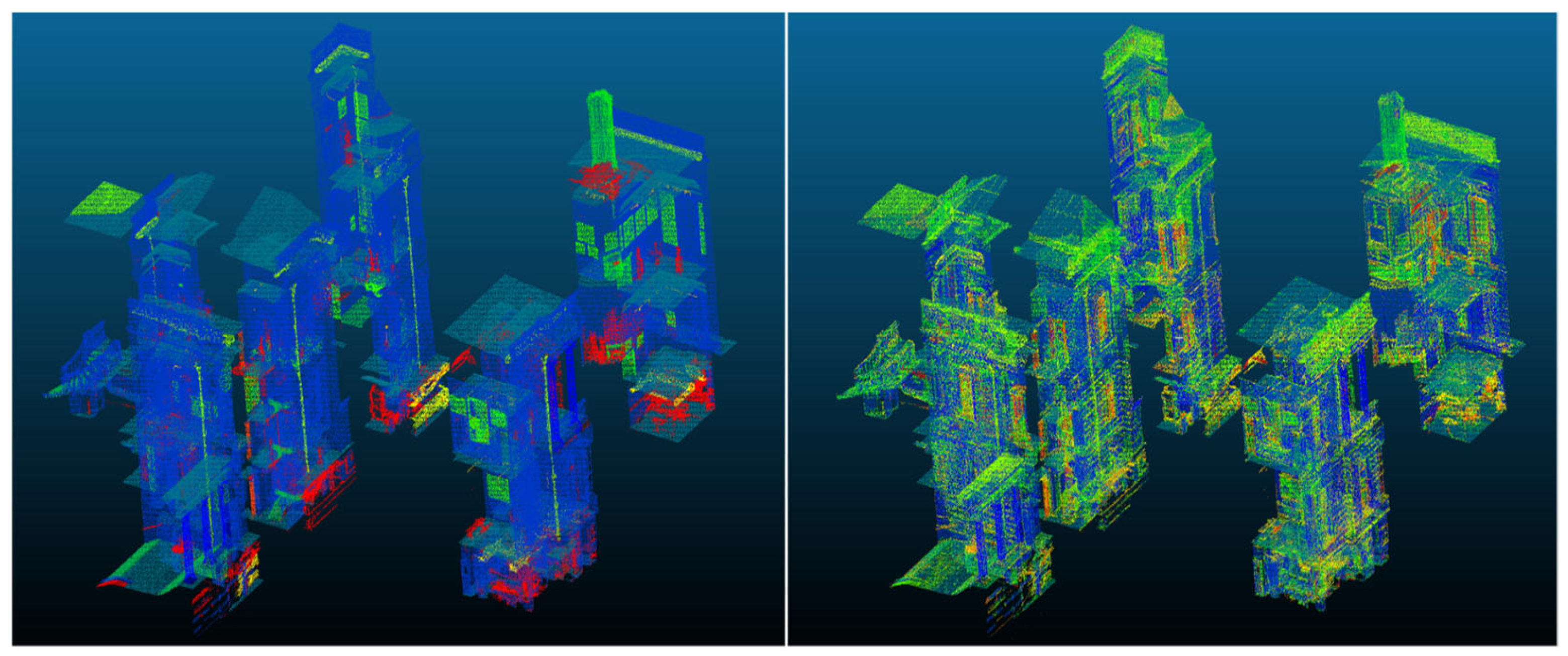
By contrast, minority classes and those whose defining features manifest at scales finer than 50 mm tended to be misclassified. This includes categories such as EF_70 (Electrical, power and lighting functions), EF_75 (Communication, security, safety, and protection functions) and EF_50 (Waste disposal functions). Figure 7 illustrates the Level 1 segmentation results in comparison of ground truth with the predicted results.

Figure 7.
Random Forest Level 1 results comparison (Left: ground truth; Right: Level 1 prediction).
As Table 4 indicates, macro-level metrics underscore the overall difficulty encountered at L1, with a macro-averaged precision of 21.2% and a macro-averaged recall of 44.5%. Although the weighted average precision appears higher (79.1%), the corresponding recall is only 32.0%, illustrating that performance is dominated by the few majority classes with comparatively large numbers of points.
Table 4.
Random Forest performance metrics at Level 1.
This discrepancy highlights a key limitation of enforcing a uniform classification tier for structurally dissimilar elements. EF_25 (Wall and barrier elements) and EF_30 (Roofs, floor, and paving elements), for example, encompass robust geometric cues at 50 mm resolution, whereas classes like EF_70 (Electrical power and lighting functions) or EF_75 (Communications, security, safety, and protection functions) may rely on fine-scale patterns not readily observable at this sampling interval. In addition, confusion matrices indicate that elements of EF_25 (Walls and barriers) are frequently mislabelled as EF_20 (Structural elements) or EF_40 (Signage, fittings, furnishings, and equipment), suggesting that the reduced spatial resolution makes it difficult for the classifier to capture subtle curvature or texture differences.
Overall, the L1 results confirm that, while the hierarchical pipeline can broadly separate walls or floors from smaller-scale elements, it faces considerable difficulties in consistently identifying classes whose dominant geometric characteristics exist below the subsampling threshold.
3.2. Full Dataset Level 2 Results
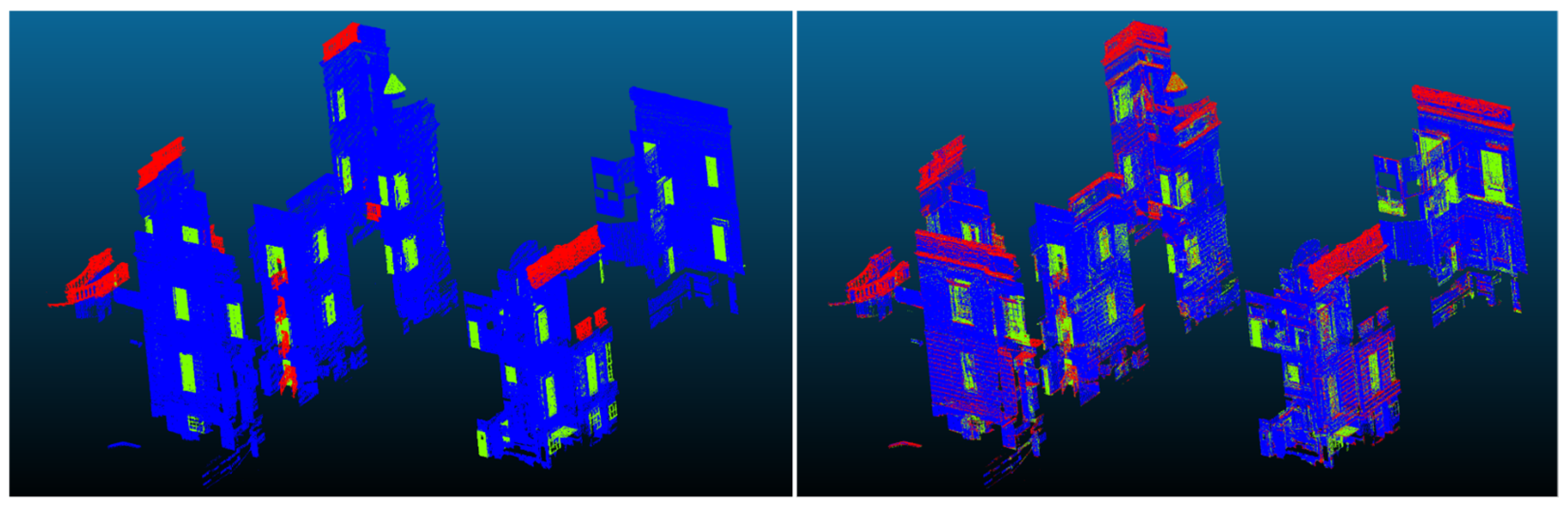
At the second level (L2), each top-level category is subdivided into its constituent child labels, and an independent classifier is trained on points within that category using a 20 mm subsampling. The intention is that focusing on a narrower set of classes at a higher resolution will result in more accurate segmentation. Figure 8 shows the Level 2 results of Random Forest implementation for the segmentation of Level 2 class building objects. The EF_25 (Wall and barrier elements) classifier, for instance, aims to discriminate between EF_25_10 (Walls), EF_25_30 (Openings), and EF_25_55 (Barriers).
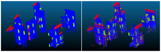
Figure 8.
Random Forest Level 2 EF_25 classifier results (Left: ground truth; Right: prediction).
Table 5 illustrates the substantial improvement in performance, with a macro-average precision of 57.5% and a macro-average recall of 71.3%. Overall accuracy stands at 75.4%. Precision for EF_25_10 (Walls) is particularly high (92.7%), suggesting that the 20 mm resolution effectively captures the relatively large planar surfaces. By contrast, EF_25_30 (Openings) and EF_25_55 (Barriers) exhibit lower precision and recall, presumably reflecting their smaller spatial footprints and fewer annotated training examples.
Table 5.
Random Forest performance metrics at Level 2, EF_25 Classifier.
Similar patterns of performance were observed for other key L2 classifiers, such as EF_30 (Roofs, floors, and paving elements). Although the principal categories, including EF_30_10 (Roofs) or EF_30_20 (Floors), were identified successfully, certain subtypes, such as EF_30_60 (Pavements) or EF_30_30 (Decks), were more prone to misclassification due to partial overlap in their geometric signatures or limited representation in the dataset. The classifier for EF_35 (Stairs and ramps) performed well for EF_35_10 (Stairs), potentially due to the distinctive geometry of steps. However, classes that appear visually or geometrically similar, such as EF_40_10 (Signage) and EF_40_30 (Furnishings), display more erratic precision and recall scores, reflecting either small sample sizes or insufficiently discriminatory features at 20 mm.
It is notable that some parent classes have few or no subdivisions at L2 and therefore do not require a separate classifier. For instance, a parent label comprising only a single child label logically imposes no further decision boundary. Where multi-label distinctions exist, however, the 2 cm resolution generally yields more pronounced geometric cues than are available at 5 cm, thus ameliorating misclassification tendencies.
3.3. Full Dataset Level 3 Results
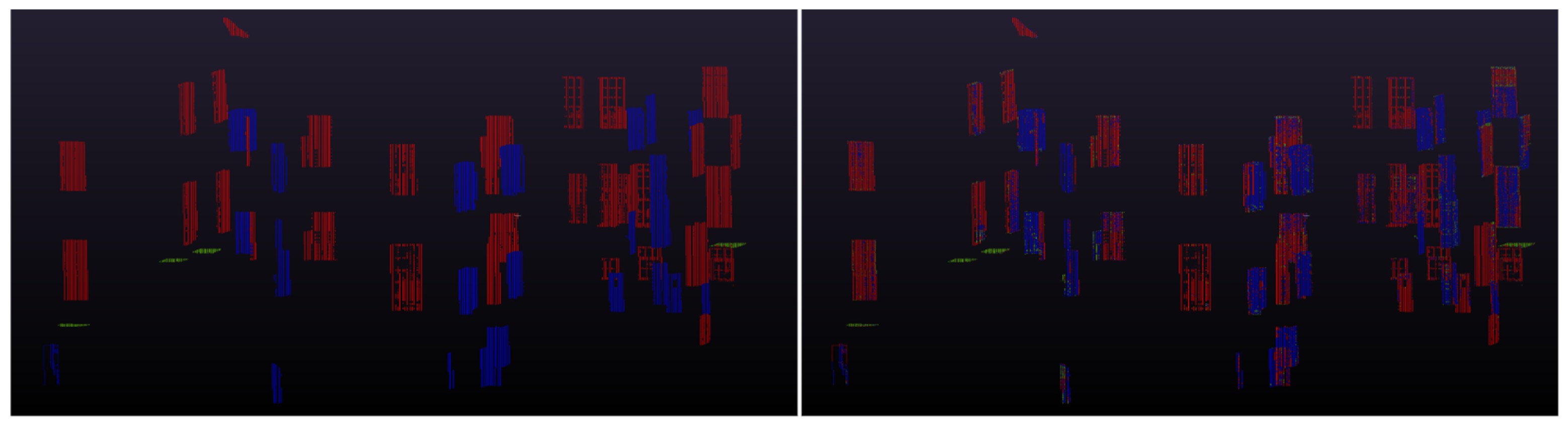
The third and finest classification level (L3) relies on a 5 mm resolution dataset, covering those elements that warrant exceptionally detailed point-level geometry. One such example, as shown in Figure 9, is EF_25_30 (Openings), which is further subdivided into EF_25_30_25 (Windows), EF_25_30_95 (Vents), and EF_25_30_97 (Doors), among other potential subclasses.
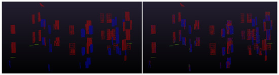
Figure 9.
Random Forest Level 3 EF_20_30 classifier result (Left: ground truth, Right: prediction).
Table 6 summarises selected metrics for EF_25_30 (Openings), showing a macro-average precision of 62.1% and recall of 80.4%, leading to a macro-average F1 score of 65.8%. These figures suggest a distinctly improved capacity to separate windows from doors and vents at the finer spatial scale, despite the added computational burden.
Table 6.
Random Forest performance metrics at Level 3, EF_25_30 classifier.
Notwithstanding these advances, L3 classification on large volumes of data presents acute hardware limitations. Notably, the classifier for EF_25_10 (Walls) could not be completed due to an out-of-memory error, as its training set exceeded 100 million points, far surpassing the capacity of the available computational resources. This indicates that while the hierarchical method can, in principle, achieve fine-grained segmentation, practical restrictions must be carefully managed, either by more aggressive subsampling, distributed computing frameworks or alternative feature engineering strategies.
The L3 results reinforce the trend observed at L2: finer resolutions improve the model’s ability to discern elements with subtle geometric differences. Nonetheless, the computational overhead grows significantly at each resolution level, emphasising the importance of scalability planning and rigorous system resource management.
4. Discussion
This research experimented with the applicability of hierarchical classification for segmenting extensive heritage-building point clouds, using a multi-level design (L1, L2, and L3) that maps specific Uniclass labels to fixed spatial resolutions. The study proceeded sequentially, beginning with the conceptual framework—namely, mapping broad categories onto coarser sizes and progressively refining labels at higher resolution—and culminating in a detailed quantitative and qualitative evaluation of classification performance. Although the overarching structure allowed for reduced computational complexity and localised classifier decisions, the findings also revealed several key limitations that inform a critique of the design and point towards potential avenues for improvement.
Initially, the experimental setup involved defining Uniclass-based classes and deciding how to distribute them across three hierarchical levels. At L1, a coarse sampling resolution of 50 mm was used to distinguish top-level categories such as EF_25 (Walls and Barriers) or EF_30 (Roofs, Floors and Paving). This strategy was adopted to ease computational load by subsampling the data at an early stage. Once the classifier had assigned points to an L1 category, those points were passed to the L2 level at 20 mm resolution for more refined classification. Ultimately, finer-grained elements (e.g., EF_25_30 subcategories such as doors or vents) would be handled at L3 with a resolution of 5 mm.
Although this approach successfully separated some large, planar features at L1—most notably walls and floors—the results showed that classes whose discriminative properties manifest at smaller scales (for example, fire safety devices or ventilation systems) were often misclassified. Key descriptors such as surface normal, curvature, or planarity, when computed on 50 mm neighbourhoods, proved insufficiently distinctive for many smaller, detailed elements. This limitation was aggravated by severe class imbalance: EF_25 encompassed a vast majority of the points, whereas categories like EF_70 (Electrical power and lighting) or EF_75 (Communication, security, safety, and protection) contained comparatively few points. Even after oversampling minority categories via SMOTE and under-sampling with ENN, these classes remained difficult to identify accurately at L1. From these results, three principal issues emerged:
- 1.
- Fixed-Scale Classification.This study highlighted that forcing certain classes to be recognised at a coarse resolution can be inherently restrictive. While some elements (e.g., walls) can be differentiated at 50 mm point spacing, others require finer granularity. This mismatch between class complexity and sampling resolution meant that classes with crucial small-scale features were effectively overlooked or merged with other categories.
- 2.
- Semantic Overlap at Coarse Resolutions.Certain Uniclass classes are semantically distinct but appear nearly identical in coarse geometric data. The confusion between EF_30 (Roofs, floors, and paving) and EF_35 (Stairs and ramps) at L1 illustrates this point: both can present similarly planar or inclined surfaces at 50 mm resolution. The hierarchical approach compels a strict decision at each level, so once a misclassification occurs, errors cascade downward.
- 3.
- Single-Scale Feature Extraction.The current workflow employs fixed-scale geometric descriptors for each classifier. In reality, many architectural objects exhibit structure at multiple scales. A window frame, for instance, may have distinctive large-scale outlines (visible at tens of centimetres) and small-scale details (hinges or handles) that require millimetric resolution. Restricting each classifier to a single neighbourhood size therefore prevents the model from leveraging multi-scale cues that could clarify borderline cases.
Moving from L1 to L2 and L3 addressed some of these shortcomings. At finer resolutions, classes featuring subtle differences became easier to distinguish. Nonetheless, new challenges arose, particularly the escalating memory and computational costs associated with training multiple random forest models on hundreds of millions of points. For EF_25_10 (Walls) at L3, out-of-memory errors halted the classification process, revealing that memory consumption can spiral as resolution grows and classifier subsets expand. This underscores the need for out-of-core algorithms or mini-batch approaches that can handle large datasets incrementally without overwhelming system resources.
Further complicating the workflow is the occurrence of single-child branches in the Uniclass hierarchy (e.g., EF_37 → EF_37_17, EF_50 → EF_50_30), which often makes fine-grained classification redundant at L2 or L3. In such cases, the L1 decision effectively determines all subsequent labels. Consequently, the L1 classifier is expected to separate complex and potentially subtle elements (like lighting equipment) at a coarse resolution, which is often infeasible. Moreover, comparisons with the Milan Cathedral study [3] illuminate how a carefully crafted hierarchy can mitigate these pitfalls. Adopting broader classes at L1 (e.g., pavement, wall, column) ensures a reliably high F1-score at the top level, thereby providing relatively pure subsets for subsequent layers.
A further overarching concern is the suitability of Uniclass itself for machine learning tasks. The system was developed for architectural design and construction documentation [25], closely tied to RIBA work stages rather than point cloud geometry. Hence, many classes do not neatly conform to morphological or topological cues. For instance, a door or window can be structurally similar to a subset of the wall, depending on the resolution in use. Observations from the experiment indicate that Uniclass categories may be too granular in certain areas (leading to severe class imbalance) and insufficiently differentiable in others. Although Uniclass corresponds well to standard building processes, it appears less optimal for direct use in a purely geometry-driven classification model.
It is worth emphasising that the random forest algorithm itself is not the primary constraint: where class distinctions were genuinely present in the feature space, the models performed appropriately, mirroring the patterns revealed by dimensionality reduction. Rather, the main barriers stem from mismatches between geometric scale, class semantics and the inherent multi-scale nature of heritage building components. While a hierarchical structure remains a sensible approach for organising large-scale datasets and reducing memory requirements, it should be accompanied by nuanced design choices—specifically multi-scale feature extraction, suitably broad classes at the top levels, and integrated strategies for balancing minority categories.
5. Conclusions
This study has demonstrated the feasibility and practical value of applying a hierarchical Random Forest classification pipeline to the semantic segmentation of large-scale point cloud data in the context of Historic Building Information Modelling (HBIM). A key contribution lies in the operationalisation of the Uniclass Element/Function (EF) table—a UK construction industry standard—as a multi-level ontological framework for guiding semantic classification. By embedding this taxonomy into the machine learning workflow, the study proposes a standards-aligned approach to generating machine-readable and semantically coherent outputs that better support interoperability within HBIM environments.
An additional innovation was the development of a bespoke point cloud annotation workflow using CloudCompare, specifically designed to overcome the limitations of conventional labelling tools when applied to dense, high-volume heritage datasets. This method enabled the structured creation of training datasets aligned with the Uniclass hierarchy, resolving practical issues around interoperability and annotation granularity that have previously hindered scalable segmentation efforts. In doing so, this study addresses a long-standing gap in HBIM workflows—providing a replicable approach that is both technically viable and openly accessible through widely used open-source tools.
The experimental results confirm that hierarchical classification is well-suited to the semantic and geometric complexity of cultural heritage assets. However, performance at finer classification levels (e.g., Level 3, with 5 mm resolution) was constrained by class imbalance, computational overhead, and geometric feature degeneracy. Certain Uniclass classes consistently underperformed due to sparse representation in the training data and ambiguous morphology in the point cloud. These outcomes highlight the limitations of applying fixed, top–down taxonomies to organically formed, irregular architectural features, particularly in heritage contexts where structural elements often deviate from modern construction norms.
Moreover, this study underscores the urgent need for more scalable learning strategies. Memory limitations and the computational cost of feature engineering impeded the full exploration of hyperparameter spaces. Future work must therefore consider distributed training frameworks and out-of-core learning methods that can accommodate the scale of modern heritage datasets without sacrificing model performance. In parallel, while hand-crafted geometric features served as an effective baseline, alternative learning architectures, particularly deep learning models such as PointNet or Point Transformer, may offer greater generalisation capacity by learning features directly from raw spatial data. Considering the findings, several directions for future research are proposed:
Firstly, multi-scale feature integration with computing geometric features at multiple spatial radii may enhance model performance by capturing both local architectural detail and broader contextual geometry, which is particularly relevant for differentiating features like pilasters versus full-length columns. Secondly, adaptation of the hierarchical taxonomy by simplifying or refining higher-level Uniclass categories, especially where classes were found to be geometrically indistinct or semantically overlapping, could reduce error propagation and improve classification robustness. Thirdly, scalable learning strategies through developing out-of-core, mini-batch, or distributed training pipelines will be critical for enabling classification on full-resolution heritage datasets that exceed in-memory processing capacity. Fourthly, exploration of deep learning models via investigating the use of neural architectures, such as PointNet, Point Transformer, or graph convolutional networks, may eliminate the dependency on manually engineered features and yield better generalisation across complex, irregular forms. Finally, taxonomy refinement for heritage applications with reassessment of the suitability of certain Uniclass EF categories, particularly those that consistently underperformed due to sparse representation or geometric ambiguity, could lead to a more heritage-sensitive classification structure through class merging or redefinition.
In summary, this study delivers a unique contribution to the field by aligning a hierarchical machine learning approach with a nationally standardised classification schema, while also establishing a replicable labelling and training methodology suited to the scale and complexity of heritage point cloud datasets. These contributions lay the groundwork for more semantically robust and scalable HBIM segmentation workflows and open new avenues for integrating ontological classification into digital heritage documentation practices.
Author Contributions
Conceptualization, A.G. and Y.A.; methodology, A.G. and Y.A.; software, A.G.; validation, A.G. and Y.A.; formal analysis, A.G.; investigation, A.G. and Y.A.; resources, A.G. and Y.A.; data curation, A.G.; writing—original draft preparation, A.G.; writing—review and editing, Y.A.; visualization, A.G.; supervision, Y.A.; project administration, Y.A. All authors have read and agreed to the published version of the manuscript.
Funding
This research received no external funding.
Data Availability Statement
The data presented in this study are available on request from the corresponding author due to (authors do not have RMG permission to share).
Conflicts of Interest
The authors declare no conflict of interest.
References
- Pierdicca, R.; Paolanti, M.; Matrone, F.; Martini, M.; Morbidoni, C.; Malinverni, E.S.; Frontoni, E.; Lingua, A.M. Point Cloud Semantic Segmentation Using a Deep Learning Framework for Cultural Heritage. Remote Sens. 2020, 12, 1005. [Google Scholar] [CrossRef]
- Grilli, E.; Farella, E.M.; Torresani, A.; Remondino, F. Geometric Features Analysis for the Classification of Cultural Heritage Point Clouds. ISPRS Int. Arch. Photogramm. Remote Sens. Spat. Inf. Sci. 2019, XLII-2/W15, 541–548. [Google Scholar] [CrossRef]
- Teruggi, S.; Grilli, E.; Russo, M.; Fassi, F.; Remondino, F. A Hierarchical Machine Learning Approach for Multi-Level and Multi-Resolution 3D Point Cloud Classification. Remote Sens. 2020, 12, 2598. [Google Scholar] [CrossRef]
- Zhang, K.; Teruggi, S.; Ding, Y.; Fassi, F. A Multilevel Multiresolution Machine Learning Classification Approach: A Generalization Test on Chinese Heritage Architecture. Heritage 2022, 5, 3970–3992. [Google Scholar] [CrossRef]
- Underwood, J.; Isikdag, U. (Eds.) Handbook of Research on Building Information Modeling and Construction Informatics: Concepts and Technologies; Advances in Civil and Industrial Engineering; IGI Global Scientific Publishing: Hershey, PA, USA, 2010. [Google Scholar] [CrossRef]
- NBS. NBS Uniclass. Unified Construction Classification. Available online: https://www.thenbs.com/our-tools/uniclass-2015 (accessed on 30 March 2025).
- Goodfellow, I.; Bengio, Y.; Courville, A. Deep Learning; Adaptive Computation and Machine Learning; The MIT Press: Cambridge, MA, USA, 2016. [Google Scholar]
- Xue, D.; Cheng, Y.; Shi, X.; Fei, Y.; Wen, P. An Improved Random Forest Model Applied to Point Cloud Classification. IOP Conf. Ser. Mater. Sci. Eng. 2020, 768, 072037. [Google Scholar] [CrossRef]
- Höhle, J. Automated Mapping of Building Facades by Machine Learning. ISPRS Int. Arch. Photogramm. Remote Sens. Spat. Inf. Sci. 2014, XL–3, 127–132. [Google Scholar] [CrossRef]
- Grilli, E.; Dininno, D.; Petrucci, G.; Remondino, F. From 2D to 3D Supervised Segmentation and Classification for Cultural Heritage Applications. ISPRS Int. Arch. Photogramm. Remote Sens. Spat. Inf. Sci. 2018, XLII–2, 399–406. [Google Scholar] [CrossRef]
- Grilli, E.; Özdemir, E.; Remondino, F. Application of Machine and Deep Learning Strategies for the Classification of Heritage Point Clouds. ISPRS Int. Arch. Photogramm. Remote Sens. Spat. Inf. Sci. 2019, XLII-4/W18, 447–454. [Google Scholar] [CrossRef]
- Croce, V.; Caroti, G.; Piemonte, A.; De Luca, L.; Véron, P. H-BIM and Artificial Intelligence: Classification of Architectural Heritage for Semi-Automatic Scan-to-BIM Reconstruction. Sensors 2023, 23, 2497. [Google Scholar] [CrossRef] [PubMed]
- Wang, L.; Liu, Y.; Zhang, S.; Yan, J.; Tao, P. Structure-Aware Convolution for 3D Point Cloud Classification and Segmentation. Remote Sens. 2020, 12, 634. [Google Scholar] [CrossRef]
- Qi, C.R.; Su, H.; Mo, K.; Guibas, L.J. PointNet: Deep Learning on Point Sets for 3D Classification and Segmentation. arXiv 2017. [Google Scholar] [CrossRef]
- Belhi, A.; Bouras, A.; Al-Ali, A.K.; Foufou, S. A Machine Learning Framework for Enhancing Digital Experiences in Cultural Heritage. J. Enterp. Inf. Manag. 2020, 36, 734–746. [Google Scholar] [CrossRef]
- Condorelli, F.; Rinaudo, F.; Salvadore, F.; Tagliaventi, S. A Neural Networks Approach to Detecting Lost Heritage in Historical Video. ISPRS Int. J. Geo Inf. 2020, 9, 297. [Google Scholar] [CrossRef]
- Tibaut, A.; Guerra De Oliveira, S. A Framework for the Evaluation of the Cultural Heritage Information Ontology. Appl. Sci. 2022, 12, 795. [Google Scholar] [CrossRef]
- ISO 19650-1:2018; Organization and Digitization of Information About Buildings and Civil Engineering Works, Including Building Information Modelling (BIM)—Information Management Using Building Information Modelling. BSI Group America: Herndon, VA, USA, 2018.
- RMG. Queens House. Available online: https://www.rmg.co.uk/queens-house (accessed on 9 April 2025).
- Withers, S. Canaletto: Synthetic Compositions of Maritime Greenwich. Archit. Des. 2023, 93, 104–111. [Google Scholar] [CrossRef]
- Delman, R. The Queen’s House before Queen’s House: Margaret of Anjou and Greenwich Palace, 1447–1453. R. Stud. J. 2021, 8, 6–25. [Google Scholar] [CrossRef]
- Che, E.; Jung, J.; Olsen, M.J. Object Recognition, Segmentation, and Classification of Mobile Laser Scanning Point Clouds: A State-of-the-Art Review. Sensors 2019, 19, 810. [Google Scholar] [CrossRef] [PubMed]
- Silla, C.N.; Freitas, A.A. A Survey of Hierarchical Classification across Different Application Domains. Data Min. Knowl. Discov. 2011, 22, 31–72. [Google Scholar] [CrossRef]
- CloudCompare. CloudCompare. 2025. Available online: https://www.cloudcompare.org (accessed on 20 January 2025).
- Delany, S. Uniclass 2015: As It Lives and Breathes. 17 June 2016. Available online: https://www.slideshare.net/slideshow/uniclass-2015-as-it-lives-and-breathes-empowering-you-in-a-bim-world/63178257 (accessed on 29 December 2024).
Disclaimer/Publisher’s Note: The statements, opinions and data contained in all publications are solely those of the individual author(s) and contributor(s) and not of MDPI and/or the editor(s). MDPI and/or the editor(s) disclaim responsibility for any injury to people or property resulting from any ideas, methods, instructions or products referred to in the content. |
© 2025 by the authors. Licensee MDPI, Basel, Switzerland. This article is an open access article distributed under the terms and conditions of the Creative Commons Attribution (CC BY) license (https://creativecommons.org/licenses/by/4.0/).