1. Introduction
It has been known for over three decades that mice produce ultrasonic courtship vocalizations [
1]. Specific pitch patterns are characterized by short, repeating monochromatic vocalizations with silent gaps in between [
2]. The production of ultrasonic vocalizations in mammals has a communicative role [
3,
4,
5,
6,
7]. A number of studies have shown that mice produce ultrasonic vocalizations in at least two situations: Pups produce “isolation calls” when cold or when removed from the nest [
8,
9], while males emit ultrasonic vocalizations in the presence of females or when they detect female urinary pheromones [
3]. It has also been observed that females in oestrus are attracted to vocalizing males, thus facilitating the process of reproduction [
10]. Several studies use the term “courtship vocalizations” [
7,
11,
12,
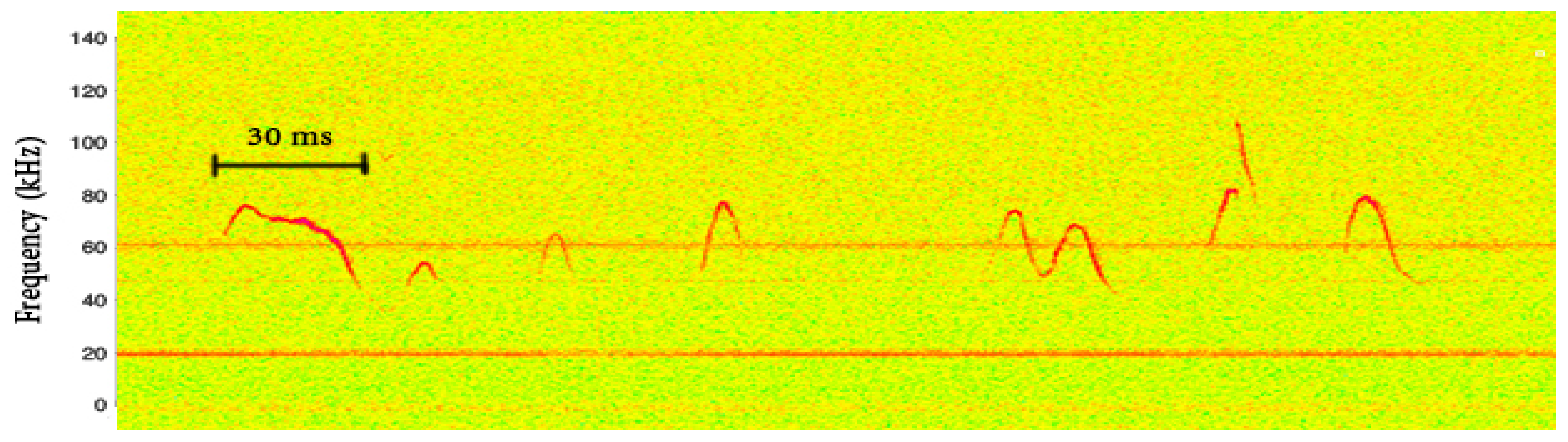
13]. It is known that these vocalizations are mainly monochromatic and appear in sequences of small bursts with approximately 30 ms of silent gaps in between [
4]. These small bursts are typically called “phonemes”. A spectrogram of such a sequence is presented in
Figure 1. The vertical red lines indicate the points where phonemes were manually segmented.
As described by Holy and Guo [
3], murine vocalizations fall into two major groups: a group consisting of “modulated” pitch contours and a group containing “pitch jumps”. The frequency trace of the vocalization in the “pitch jump” group contains one or two discontinuities. They actually report three types of phonemes as subcategories. Similar phonemes appear in our dataset and will be presented in
Section 3.
The concept of using a representation of the pitch tracks as feature vectors and the use of machine learning techniques can also be found in [
7,
11,
14,
15,
16]. In [
14], Musolf et al. used the Avisoft software to extract 25 features including, among others, frequency values indicating the start, center, and end frequency of the pitch track, frequency at peak energy, as well as the vocalization duration. They performed dimensionality reduction using principal component analysis and applied supervised techniques such as support vector machines. The phonemes of male mice were classified into seven categories (five modulated and two pitch jumps). In [
11], the authors suggest four categories for the repertoire of the wild house mice. Two belong in the modulated and two in the pitch jump group.
Since the phonemes of male vocalizations are repeating, Holy and Guo introduced the term “male mice songs” [
3]. The term “song” has been widely used in animal vocalization research, including on birds, frogs, whales, and bats [
17,
18,
19,
20]. The terms “calls”, “phonemes”, “motifs”, and “phrases” relate to the structure of a song in a similar way to the songs in music [
21].
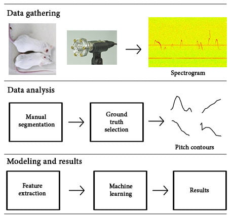
In this study, we apply two unsupervised machine learning methods for clustering the ultrasonic vocalizations of young male BALB/c mice in the presence of a female in oestrus (BALB/c is an albino, laboratory-bred strain of the house mouse from which a number of common substrains are derived; having initially been bred in New York in 1920, over 200 generations of BALB/c mice are now distributed globally, and they are among the most widely used inbred strains used in animal experimentation). More precisely, we chose to apply the k-means method mainly because not only it is easy to understand and implement, but it is also one of the most widely used algorithms for clustering. Since we use k-means, which is a distance-based method, we normalized the data (range between 0 and 1). Furthermore, we chose to apply an additional method (agglomerative clustering) for the verification of our results. The agglomerative clustering results become more interesting when they are visualized as a dendrogram. The added value of such a method is that one can explore subclusters, which can give insights and a better understanding of the data. We show that the ultrasonic vocalizations can be categorized into nine distinct categories based on their acoustical features. This fact reinforces the claim that there is a distinct repertoire of “syllables” or “phonemes” and comprises the main contribution of this work.
The rest of the paper is organized as follows: In
Section 2, the methodology pertaining to data acquisition, signal analysis, and dataset formation along with the machine learning techniques used for clustering, is presented. In
Section 3, remarks on our results are made, followed by a discussion and concluding remarks in
Section 4.
2. Materials and Methods
2.1. Experimental Conditions and Recordings
The BALB/c mice used for our experiments were three months old, having been born and raised in captivity at the Biology Department of the University of Crete (Heraklion, Crete, Greece, EL91-BIObr-09/2016, Athanassakis I., Kourouniotis K., Lika K.). During the experiments, a certain number of mice were transferred to an adjacent noise-insulated lab equipped with the ultrasonic recording devices (females being in oestrus at the time of the recordings and approximately at the same estrus stage).
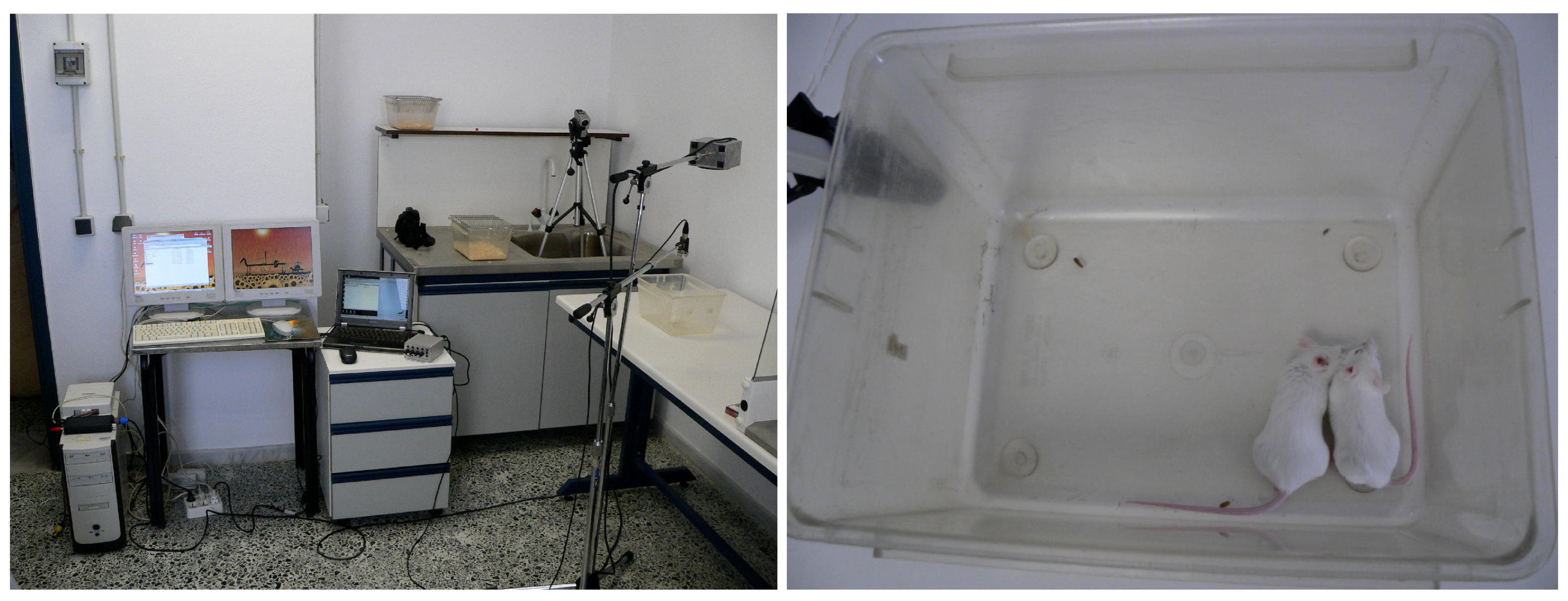
All the experiments were conducted with the mice in a container of dimensions of 30 × 15 × 15 cm. The ultrasonic condenser microphone (Model CM16/CMPA, Avisoft Bioacoustics, Berlin, Germany) was placed on top of the container at a distance of approximately 30 cm (
Figure 2).
Signal acquisition was done through Ultra Sound Gate (Avisoft Bioacoustics, Berlin, Germany), which performs analog to digital conversion, signal conditioning, and provides polarizing voltage to the ultrasonic condenser microphone. It comes with built-in anti-aliasing filters, and its A/D converters are of a Delta–Sigma architecture. It can amplify the signal up to 40 dB, while its sampling frequency can reach 750 kHz at 8 bit resolution. We used a 250 kHz sampling rate at a 16 bit resolution, and the recording was done in the SASLab software environment (Avisoft Bioacoustics, Berlin, Germany).
2.2. Data and Pitch Contour Extraction
The total duration of all the ultrasonic recordings undertaken sum up to about 2.5 h. Several recording sessions were undertaken, and more than 15 different mice were used. The recordings were manually segmented, resulting in a dataset of 179 phonemes.
For each phoneme extracted from a series of audio recordings, contours were formed from the detected vectors of the monochromatic frequencies. The pitch contour of the ultrasonic monochromatic vocalizations is formed from overlapping frames, where in each frame the most prominent frequency is detected through the FFT. (Here, we use the term “pitch” loosely since this term is meant to be used for the perceived sensation of frequency). The amplitude of the prominent frequency, compared to the remaining spectrum, is significantly higher, as shown in
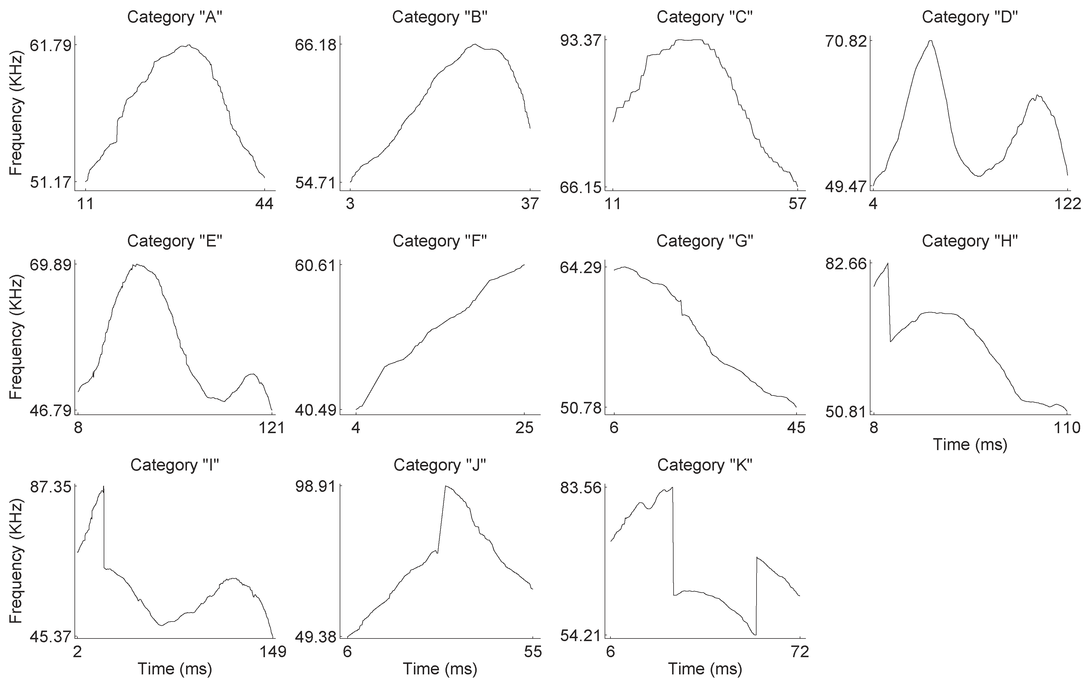
Figure 3, and thus, it is relatively easy to identify a unique pitch candidate for each frame. After the estimation of pitch candidates, a post-processing procedure is applied in order to correct some errors, appearing mainly in the noisiest parts of the signal. All pitch contour shapes were manually categorized into one of the representative categories depicted in
Figure 4 (see also
Section 3).
2.3. Feature Extraction
The approach taken here was to define a set of 14 features that pertain to: (a) the frequencies themselves and (b) the temporal positions of some designated time-points across the phonemes. Thus, the features are: (1) the beginning frequency, (2) the end frequency, (3) the mean frequency, (4) the standard deviation of the frequency, (5–6) the middle frequency (value and position), (7–8) the first quartile of the frequency (value and position), (9–10) the second quartile of the frequency (value and position), (11–12) the third quartile of the frequency (value and position), and (13–14) the fourth quartile of the frequency (value and position).
The raw frequency values derived from the pitch track are normalized because we use distance metrics (i.e., Euclidean distance) in the k-means method.
The decision on the number and nature of parameters was made with robustness and low dimensionality in mind. The selected parameters effectively attribute the contour shape of each vocalization. Descriptors based on the signal’s acoustic characteristics were not used (i.e., those derived from the Fourier transform, like the spectral centroid or the spectral spread).
2.4. k-Means
The k-means algorithm is repeatedly applying two operations until convergence is reached. It initially computes the distances between all data points and all the prototypes representing every cluster and assigns the data points to the cluster belonging to the closest prototype. Then, it repositions the prototypes to the mean of each cluster. The convergence criterion can be set as the condition where all of the prototypes are not significantly different from the mean values of their clusters. Another criterion can simply be a specified number of iterations. In this paper, we used the first case as a convergence criterion.
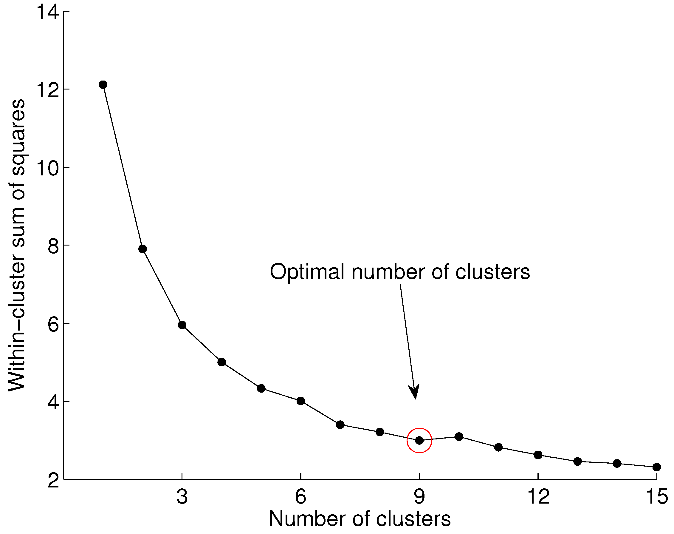
We used the elbow method for finding the optimal number of clusters. First, we compute the sum of squared errors (SSE) for
, as shown in Equation (
1), and then we look at the values of the SSE across the number of clusters. Typically, the SSE drops significantly as more clusters are added. After the optimal number of clusters for a particular problem is reached, the SSE remains relatively constant.
In Equation (
1),
k is the number of clusters,
is the number of points in cluster
r, and
is the sum of distances between all points in a cluster, given by:
A graph of the SSE against the number of clusters derived from our data is shown in
Figure 5. It is indicated that beyond nine clusters, the SSE remains relatively constant.
The k-means algorithm typically returns different results when experiments are repeated, mainly because of the randomized initialization of the prototypes. As a result, the elbow method may also return a different number of optimal clusters. To create a robust conclusion for this work, we ran our experiments 500 times, and in each run, we identified the optimal number of clusters. In our dataset, we observed that the optimal clusters for different runs were between 8 and 10. However, in the majority of runs, the method suggested 9 optimal clusters.
2.5. Agglomerative Clustering
We chose to apply agglomerative clustering [
22] to our data in order to compare the results with the widely used
k-means clustering algorithm. In addition, data can be viewed as a dendrogram, which can give a better understanding of the subclusters and the relation of the instances between pairs.
Agglomerative clustering groups the instances in a dataset with a hierarchical order. Initially, each instance is seen as a separate cluster. Then, a similarity measure is computed between all possible pairs. A linkage criterion determines pairs of instances that are grouped together within a single cluster, creating the first layer of subclusters. In a similar manner, pairs of data are linked in subclusters until all instances become one cluster. A threshold can be used in any branch of the tree to get the clustering results.
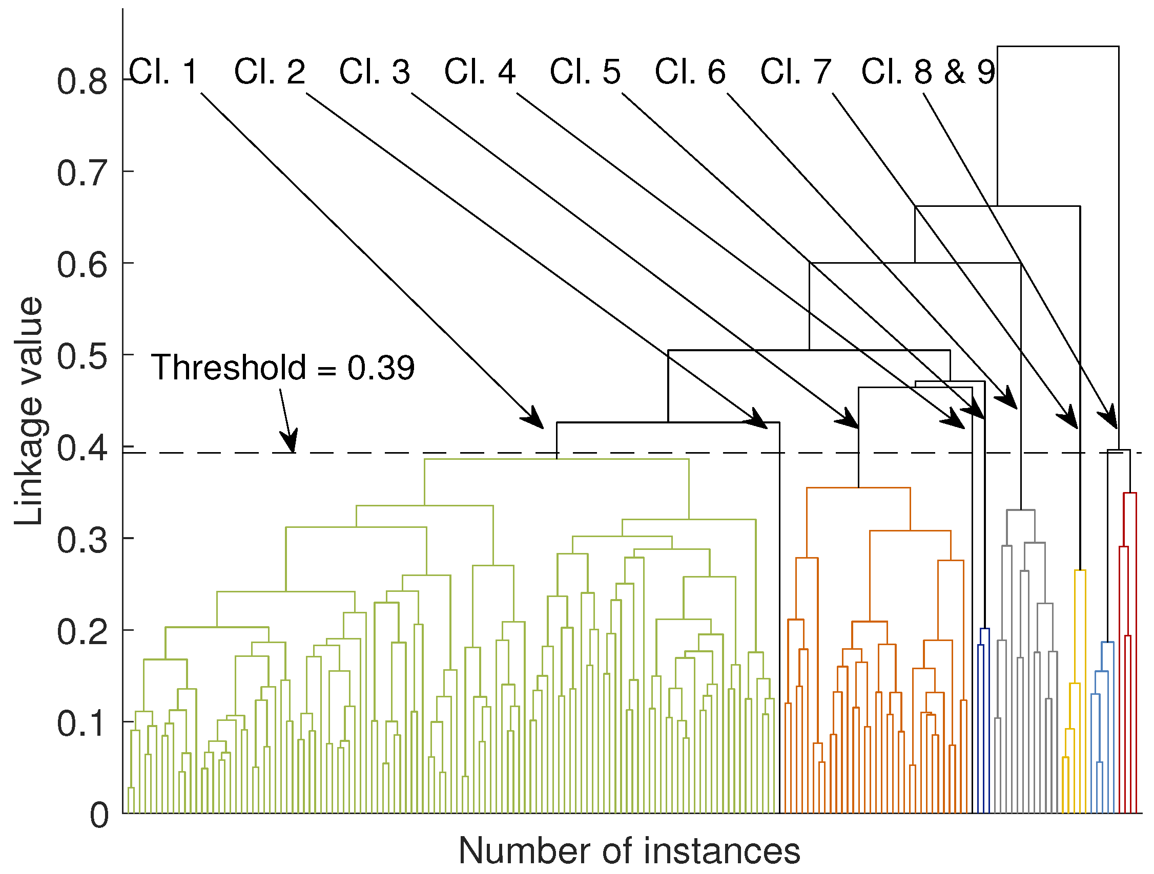
The similarity measure can be any distance, for instance, the Euclidean or Mahalanobis distance. Examples of linkage criteria include the maximum or minimum distances between pairs or other more sophisticated approaches taking into account the probabilities between distributions. A dendrogram derived from our dataset is shown in
Figure 6. We elaborate further on the outcome of the agglomerative clustering in
Section 3 and
Section 4.
3. Results
By visual inspection of the pitch contours, we identified 11 generic contour shapes, which were labeled according to their shape (see
Figure 4). In
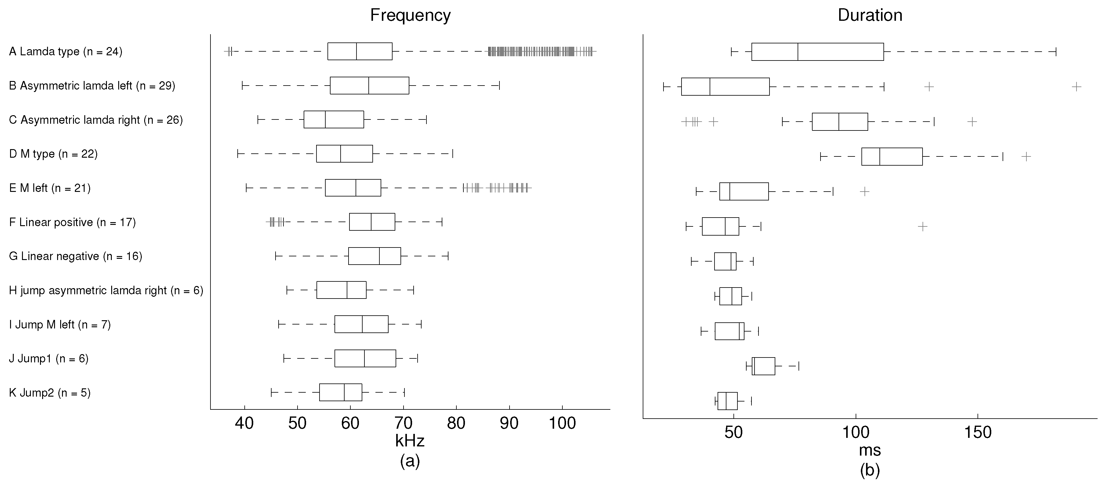
Figure 7, we present some statistics of the phonemes in each category. The ground truth here is used only to measure the performance of the unsupervised methods. Therefore, the recommended number of clusters is derived by the “elbow method”. The ground truth is not involved in the training procedure.
The phonemes fall into two general groups: those presenting some modulation without any pitch jumps and those with one or two pitch jumps. The modulated group is formed by the A–G categories, while the pitch jump group is formed by H–K categories. The number of modulated phonemes (categories A–G) is higher in the sample than the number of phonemes in the pitch jump group (categories H–K). From the mean frequency perspective, it is shown that the values in all categories are found around 60 kHz, except for category J, which has a mean frequency value of 71 kHz. The shortest mean duration of the phonemes is found in category F and the longest in category I. The mean duration is around 60 ms, except for categories D and E, which have longer durations.
In
Figure 8, mean normalized values of the 14 features for all 179 phonemes are plotted. The dots represent these values in every category and are joined with lines for better visualization. The category label (see
Figure 4) is annotated below the horizontal axis, while the vertical lines simply separate the different categories. The number of phonemes in each category is shown at the top of the figure between the separation lines. The average value for each category is pictured as a thick horizontal line. In
Section 4, we discuss further the consistency between the feature set, as shown in
Figure 8, and the results from the
k-means algorithm.
The clustering results from the
k-means algorithm for
are shown with a matching matrix in
Table 1. The rows indicate the 11 ground truth categories and the columns the k-means output. More than 80% of the A - lambda category has been assigned to cluster 9, together with the 45% of the B - asymmetric lambda left. The majority of the instances in categories C - asymmetric lambda right and G - linear negative are assigned to cluster 3 (95% and 86%, respectively), showing some similarity in their feature vectors. Similarly, 77% of the D - M type, 81% of the E - M left, and 80% of the K - jump 2 categories are assigned to cluster 1. The two categories H - jump asymmetric lambda right and I - jump M left (67% for H and 100% for I), are placed in cluster 2. The category F - Linear positive is spread in clusters 4–7.
In
Figure 6 we present a dendrogram derived from the agglomerative clustering algorithm. In order to view the several clusters of this method, it is necessary to apply a threshold to a branch of the tree, for the sub-branches to form the respective clusters. With the threshold set at 0.4 we get 9 clusters, shown with different colors in
Figure 6 (in the electronic version of the paper). The first five clusters are stemming from the same branch in the two higher levels of the tree and they contain mainly phonemes from the modulated group. The remaining four clusters are coming out from different branches of the tree and they contain phonemes mainly from the pitch jump category.
4. Discussion
In this work, we used unsupervised machine learning techniques to create clusters of phonemes that share similar characteristics. It is shown in
Figure 7 that the mean frequency of the J category is statistically higher than the average frequency among all categories. In the matching matrix (
Table 1), by comparing the
k-means outputs to the ground truth, we can see that 83% of the phonemes of the J category fall in the 8th cluster. From the matching matrix, we also observe that categories D, E, and K are seen by the
k-means mainly as one class. The mean durations of the phonemes for categories D and E are similar, although they are statistically higher than the overall mean duration (
Figure 7).
Looking at
Figure 8, we observe very similar values for the normalized means across the 14 feature values for categories D, E, and K. Similarly, from the matching matrix we see that categories C and G fall into cluster 3. The normalized mean feature values of categories A, C, and G are also statistically similar. The highest mean feature value appears in category F, and the pitch jump categories appear to have relatively lower mean feature values in relation to the total mean value across all categories.
The use of the dendrogram as a visualization and clustering technique adds some value to the understanding of the data and the hierarchy of the similarity between phonemes. It seems that if the threshold is placed at 0.39, then indeed, the agglomerative clustering returns results that are consistent with those of the
k-means algorithm, as well as with those reported in the literature [
3].
Regarding the size of the dataset used in this study, we have to remark that the number of phonemes belonging, especially, to the pitch jump group appears to be relatively small. These kinds of vocalizations were much rarer despite the fact that the collected vocalizations arose from several hours of recordings. Nevertheless, we claim that since our results are consistent with those reported in the literature, a richer dataset would have yielded similar results.
Note also that despite the fact that data were recorded both in the audio and the ultrasonic spectrum, in this study we focused primarily on the ultrasonic range. The ultrasonic phonemes, in most cases, were mainly continuous whistles with a mean duration of 500 ms. The sounds with discontinuities (denoted as jumps) are attributed to the nonlinearities of the vocal fold system, pertaining to bifurcations. Thus, in our study, the precise representation of the frequency trace (contour) was of primary concern. This is the main reason we developed the mentioned contour extraction and processing method instead of using other freely available software, such as MUPET [
23]. MUPET is a remarkable project, but its contour extraction process inspired by the workings of the human auditory system and symmetric and evenly distributed Gammatone filterbank (composed of 64 band-pass filters) that spans the whole mouse ultrasonic vocalization (USV) frequency range is not fully justified in our opinion (especially the fact that the upper and lower bounds of the frequency range is modeled by a smaller number of wider filters that are symmetric).


