A Frequency-Independent Phase Shifter

Abstract

In this paper, we utilise optimization methods to determine a frequency-independent phase shift such that two phase-shifted versions of a signal can be summed and the resulting amplitude spectrum is unchanged. A phase difference between two signals is thus defined, which remains constant for all frequencies within a given range. For the intended purpose of this study, we set the frequency range to the audible human hearing range of 16 Hz–20 kHz. We found that a new 3-stage filter method provides a variable phase shifter (i.e., ϕ = 0–360°) without the need for additional amplifiers. In addition, we present a new method that reduces the number of filters necessary, improving both the accuracy and efficiency of current techniques.

1. Introduction

Phase shifters change the output phase angle of an input signal and are thus utilised in many areas of electronics, instrumentation, and signal processing [1,2,3,4,5,6].

The most commonly used types of phase shifters are, in fact, time delayers, which introduce a frequency-independent time delay. Depending on the intended application of the phase shifter, it is important to consider how the amplitude response is affected. For example, when controlling variable response angles in a spatially distributed microphone array, microphone signals are combined and phase-shifted [7,8,9,10]. It is therefore important that the phase shift is independent of the frequency, such that the amplitude response is equal for all frequencies and the resulting amplitude spectrum of the signal is unchanged. However, such frequency-independent phase shifters are more complex in their technical design and have yet to be optimally developed. For example, a traditional phase shifter in which the phase shift is changed manually can be used to achieve a frequency-independent phase shift [1,11,12]. These methods can then be automated with the use of a programmable variable resistor [13,14,15,16,17,18]. However, they are only operational either at single frequencies [16] or specific frequency ranges, but at a lower accuracy [17]. They can also require multiple stages [18].

For a frequency-independent phase shift of 90° (π/2 in radians), a comprehensive analytical solution is given by the Hilbert Transform. The Hilbert Transform can be understood as first transforming into the frequency domain by applying a FFT and then phase-shifting all positive frequency spectral components by −90° and all negative frequency spectral components by +90°. Then, by applying the inverse FFT, a time domain phase-shifted spectrum is obtained where the amplitude spectrum is unchanged. However, this solution is purely analytical, and no straightforward implementation exists analogously in signal processing. Implementation is thus carried out by passing the signal through various stages of filters, i.e., band-pass filters and all-pass filters. Various strategies for implementation can be found that may differ greatly based on the intended application, and each has their own limitations and drawbacks. For example, [18] implements the Hilbert transform via a two-stage filter and a five-stage filter. In both cases, a flat response was achieved for a specific frequency range of ω = 55 Hz–2 kHz and a phase angle of ϕ = 34°, as well as for ω = 100 Hz–20 kHz, ϕ = −30°, respectively. This approach works well, but is costly in terms of implementation and only allows fixed phase shifts for a limited frequency range. Another approach allows for a variable phase shift, i.e., ω = 16 Hz–20 kHz, ϕ = 0–360°, by implementing a Hilbert transform via a 2 × 3-stage filter and three additional amplifiers [10]. In this approach, the added functionality and range come at further added computational costs.

It is evident that the current methods utilised to achieve frequency-independent phase shifts require substantial complexity in the technical design and involve multiple filters, thus limiting efficiency. In this paper, we utilise optimization methods to determine a frequency-independent phase shift. We describe a three-stage filter that provides a variable phase shifter, i.e., ϕ = 0–360°, without the need for additional amplifiers. In addition, we present a new method that reduces the number of filters necessary, improving on both the accuracy and efficiency of current techniques.

2. Materials and Methods

An all-pass filter is a filter that introduces a phase shift while not affecting the amplitude response of a signal. They are typically designed using operational amplifiers and discrete resistors and capacitors. See Figure 1a for an example of a first-order all-pass filter and Figure 1b for an example of a second-order all-pass filter. Note that both examples are for a phase shift variation from −180° (at 0 Hz) to 0° (at higher frequencies), where, at ω = 1/RC, the value of the phase shift is −90°.

These circuits are only operational at a single frequency, where each component is chosen specifically for a phase shift at a given frequency. If we want to adapt such a system to a phase shift for variable frequency, we have to make the circuit frequency-independent using variable components, e.g., programmable resistors and capacitors; voltage control resistors (VCR); and Junction-gate Field Effect Transistors (JFET). For an example, see Figure 2.

An all-pass filter can also be implemented digitally; see Figure 3 for an example of a digitally implemented (Figure 3a) first-order and (Figure 3b) second-order all-pass filter.

We can then use an all-pass filter to achieve a band-stop filter where the frequency range is determined by a centre frequency, ω₀, $\mathrm{and}$ $\mathrm{a}$ bandwidth, $BW$, defined by $\mathrm{the}$ $Q$-factor:

$$Q={\displaystyle \frac{{\omega }_0}{BW}}.$$

(1)

The band-stop filter is a combination of a low-pass filter and a high-pass filter with identical cut-off frequencies, corresponding to ω₀ above (see Figure 4).

A first-order all-pass band-stop filter can be used to achieve a signal with a uniform amplitude response and a phase response $\varphi$ as a function of frequency $\omega$, expressed as

$$\varphi (\omega )=-4·atan(\omega /{\omega }_0)$$

(2)

Note that the addition of the low-pass and high-pass filters results in a maximum phase shift range of 360° (i.e., −4atan).

The second-order filter allows a variable bandwidth with a phase response by introducing the Q-factor as a new parameter:

$$\varphi (\omega )=-4·atan[(\omega /{\omega }_0{)}^{-Q}]$$

(3)

See Figure 5 for the resulting phase shifts for ω₀ = 500 Hz and $Q$ = 0.5–2.0.

A combination of several such phase shifters can also be utilised. For example, one can take a phase shifter (A) of three components:

$$\begin{gathered} {\varphi }_A(\omega )=-4·atan[(\omega /{\omega }_{0,1,A}{)}^{-Q_{1,A}}]-4·atan[(\omega /{\omega }_{0,2,A}{)}^{-Q_{2,A}}] \\ -4·atan[(\omega /{\omega }_{0,3,A}{)}^{-Q_{3,A}}] \end{gathered}$$

(4)

with parameters

$${\omega }_{0,1,A}=16 Hz, {\omega }_{0,2,A}=320 Hz, {\omega }_{0,3,A}=6400 Hz,$$

and

$$Q_{1,A}=Q_{2,A}=Q_{3,A}=0.707$$

and another phase shifter (B):

$$\begin{gathered} \hspace{1em}\hspace{1em}\hspace{1em}\hspace{1em}\hspace{1em}\hspace{1em}{\varphi }_B(\omega )=-4·atan[{(\omega /{\omega }_{0,1,B})}^{-Q_{1,B}}\left]-4·atan\right[(\omega /{\omega }_{0,2,B}{)}^{-Q_{2,B}}] \\ -4·atan[(\omega /{\omega }_{0,3,B}{)}^{-Q_{3,B}}], \end{gathered}$$

(5)

with parameters

$${\omega }_{0,1,B}=35 Hz, {\omega }_{0,2,B}=700 Hz, {\omega }_{0,3,B}=\mathrm{14,000} Hz,$$

and

$$Q_{1,B}=Q_{2,B}=Q_{3,B}=0.707,$$

and obtain the total phase shift as

$$\varphi (\omega )={\varphi }_A(\omega )-{\varphi }_B(\omega ).$$

(6)

The individual $\varphi$_A($\omega$) and $\varphi$_B($\omega$) phase shifts are shown in Figure 6.

The difference in these phase shifts, $\varphi$($\omega$), is more or less constant in the 30 Hz to 6 kHz range, but exhibits substantial variation even within that range. Outside that range, the phase shift changes even more (see Figure 7).

In the following section, we describe the optimization of such filters with one or more stages, with parameters optimised numerically and analytically as well. The former method usually yields more accurate results, while the latter helps in guiding the analysis and obtaining a more detailed qualitative understanding.

3. Results

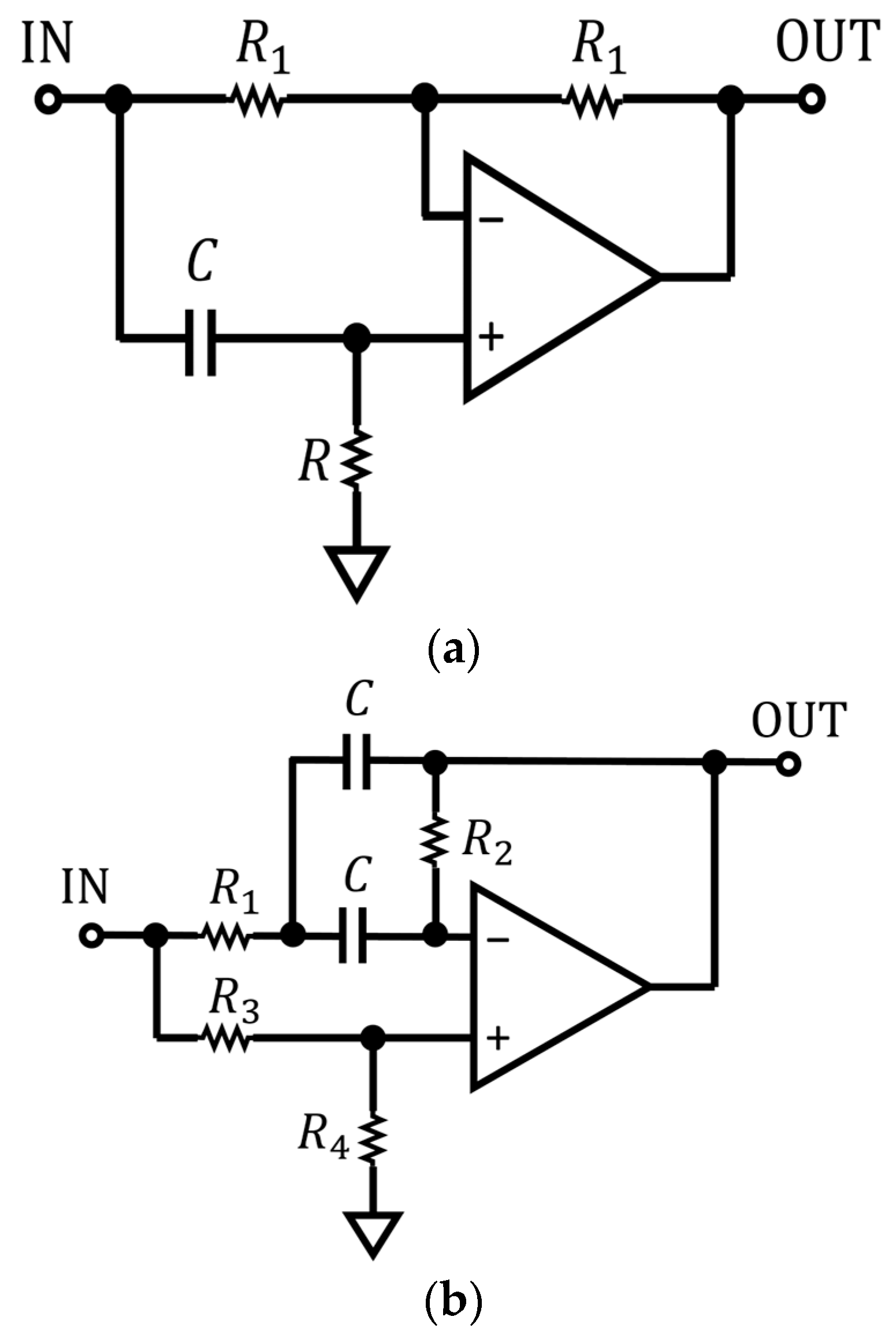
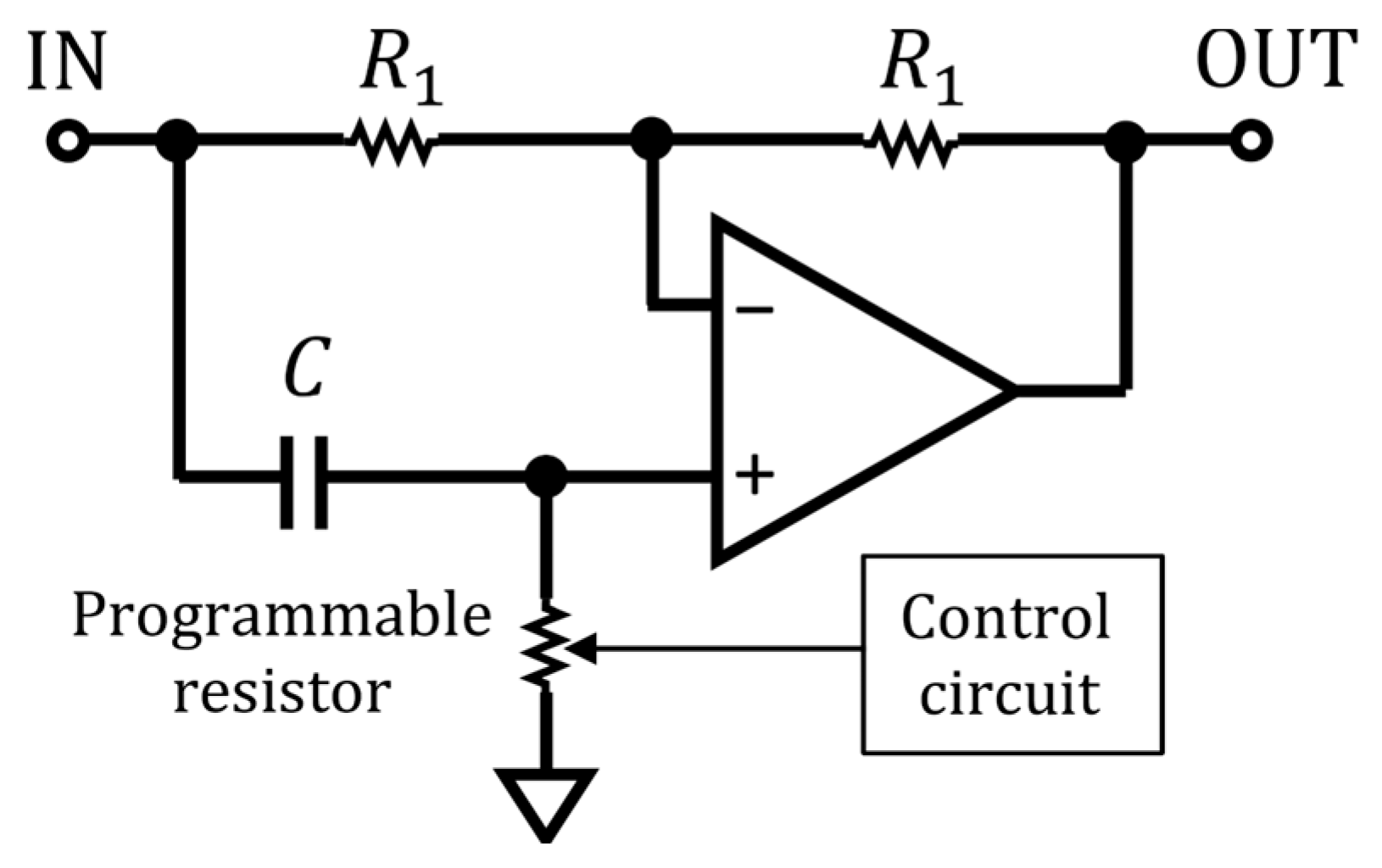
3.1. Numerical Optimization of a Single-Stage Filter

To achieve a more constant phase shift as compared to the default version discussed above, we can numerically optimise the parameters by minimising the deviation from a constant $\varphi$($\omega$) = $\varphi$₀, where $\varphi$₀ is the desired phase shift. This can be achieved by defining a penalty function and then finding its minimum as a function of the parameters. As an example, we investigated $\varphi$($\omega$) with parameters optimised for $\varphi$₀ = −π/2 when the central frequencies are unmodified and only the $Q$-factor parameters are optimised. This was achieved by utilising the ROOT Minuit2 framework (version 6.28), where a penalty function χ² was defined as the squared relative deviation of $\varphi$($\omega$) and $\varphi$₀, integrated over the relevant frequency range:

$${\chi }^{2 }={{\displaystyle \int }}_{{\omega }_{min}}^{{\omega }_{max}}{\displaystyle \frac{{({\Phi }_A(\omega )-{\Phi }_0)}^2}{{{\Phi }_0}^2}}d\omega$$

The minimal deviation (i.e., the optimal χ²) in the range defined via ${\omega }_{min}=1$ Hz and ${\omega }_{max}=$ 100 kHz was achieved with the following set of values:

$$Q_{1,A}=0.913, Q_{2,A}=0.721, Q_{3,A}=0.819$$

$$Q_{1,B}=0.807, Q_{2,B}=0.683, Q_{3.B}=0.802$$

As expected, a flatter, but still substantially oscillating $\varphi$($\omega$) was achieved compared to the previous unoptimized case, as shown in Figure 8 (focused on the important frequency range from 15 Hz to 16,000 Hz).

In contrast to this, e.g., for $\varphi$₀ = −0.259, an even flatter $\varphi$(ω) can be achieved (see Figure 9) with

$$Q_{1,A}=0.0449, Q_{2,A}=0.172, Q_{3,A}=0.169,$$

$$Q_{1,B}=0.0638, Q_{2,B}=0.189, Q_{3.B}=0.131.$$

One may note, however, that the parameters listed above have huge uncertainties. The uncertainty here means that the given parameter can be varied within an interval corresponding to the uncertainty, and the resulting χ² value, defined in terms of the variance of the relative deviation from the desired constant phase shift, will change only by up to one unit. Hence, an equally constant phase shift can be achieved with significantly different parameters, but these need to be co-varied. Thus, it is clear that the parameters can be varied in broad intervals to obtain a similar level of constantness of the phase shift. In other words, one can fix some of the parameters to almost arbitrary values, and then fit just the remaining ones. At the same time, a filter with fewer than three stages might be possible if its parameters are optimised. This suggests that instead of numerical optimization, an analytical calculation might also be feasible.

3.2. Analytic Calculations for the Single Stage Filter

To analytically investigate the form utilised in the previous section, we set two single-stage filters with the following frequency-dependent phase-shifts:

$$\varphi (\omega )=-4·atan\left[{(\omega /{\omega }_{0,A})}^{-Q}\right]-4·atan\left[{(\omega /{\omega }_{0,B})}^{-Q}\right]$$

(7)

where the central frequencies are different, but the $Q$ exponents are identical. Utilising a series expansion technique, we found a good approximation of the above function in the following form:

$$\varphi (\omega )\approx {\varphi }_A(\delta )={\varphi }_{min}+D\cdot {\delta }^2$$

(8)

with

$$\delta =ln({\displaystyle \frac{\omega }{\sqrt{{\omega }_{0,A}{\omega }_{0,B}}}}),$$

$${\varphi }_{min}=4·atan{\displaystyle \frac{1}{2}}\left\{{({\displaystyle \frac{{\omega }_{0,B}}{{\omega }_{0,A}}})}^{{\displaystyle \frac{-Q}{2}}}-{({\displaystyle \frac{{\omega }_{0,A}}{{\omega }_{0,B}}})}^{{\displaystyle \frac{-Q}{2}}}\right\},$$

and

$$D={\displaystyle \frac{4{({\omega }_{0,A}{\omega }_{0,B})}^{Q/2}({{\omega }_{0,B}}^Q-{{\omega }_{0,A}}^Q)Q^{2 }}{{{\omega }_{0,A}}^{2Q}+{{\omega }_{0,B}}^{2Q}+2{{\omega }_{0,A}}^Q{{\omega }_{0,B}}^Q}}$$

This approximation reflects that the $\varphi$(ω) function above has an exact minimum, $\varphi$_min at ω = ω_min$\equiv \sqrt{{\omega }_{0,A}{\omega }_{0,B}}$, while the second derivative is related to $D$, defined above. This can be used to estimate the level of constantness of $\varphi$($\omega$) near the minimum: the smaller the value of $D$, the more constant $\varphi (\omega )$ is within a given vicinity of ω_min.

3.3. Analytical Optimization for the Single-Stage Filter

To optimise $\varphi (\omega )$ in such a way that χ², quantifying the difference of $\varphi (\omega )$ and ϕ₀, is minimised, we can define χ² by the following integral:

$${{\displaystyle \int }}_{{\omega }_{min}}^{{\omega }_{max}}{\displaystyle \frac{{(\Phi (\omega )-{\Phi }_0)}^2}{{{\Phi }_0}^2}}d\omega$$

(9)

However, given the approximative shape (see Figure 8), this leads to a complex result. We instead define χ² via an integral on $\delta$, defined in Equation (8), instead of ω:

$${\chi }^{2 }={{\displaystyle \int }}_{{\delta }_{min}}^{{\delta }_{max}}{\displaystyle \frac{{({\Phi }_A(\delta )-{\Phi }_0)}^2}{{{\Phi }_0}^2}}d\delta$$

(10)

where

$${\delta }_{min/max}=ln({\displaystyle \frac{{\omega }_{min/max}}{\sqrt{{\omega }_{0,A}{\omega }_{0,B}}}}).$$

We find that χ² can be readily expressed in terms of the integration range ω_min and ω_max and the original parameters $Q$, ω_{0, A}, and ω_{0, B} (‘hidden’ in $D$ and ϕ_min), as:

$${\chi }^{2 }={\displaystyle \frac{3D^2({{\delta }_{max}}^5-{{\delta }_{min}}^5)-10D({{\delta }_{max}}^3-{{\delta }_{min}}^3)({\Phi }_0-{\Phi }_{min})-15({\delta }_{max}-{\delta }_{min}){({\Phi }_0-{\Phi }_{min})}^2}{{{\Phi }_0}^2}}$$

(11)

However, this expression is still complex, especially when $D$ and ϕ_min are substituted back into it.

In addition, one may observe that there is no unique minimum of this χ² even if one of the variables is fixed (see Figure 10).

These plots illustrate that there is no single strong minimum on the χ² map; instead, a valley of minima is present, and no single best set of parameters can be found. This also implies that some combinations of the parameters represent weak modes of the χ², while other combinations represent strong modes, i.e., significant parameter combinations. Further exploration into these parameter combinations is thus required.

3.4. Approximative Method for the Analytical Solution of the Single-Stage Filter

Instead of numerically minimising the above-defined χ², we explore analytical possibilities as well. Equation (8) introduces an approximate formula for ϕ(ω), expressed via auxiliary variables $\delta$, ϕ_min, and $D$, which allows us to, both directly and analytically, explore the deviation of ϕ(ω) from a given ϕ₀. On the other hand, its average can be assessed easily if the desired interval is logarithmically centred around $\delta =0$, i.e., ω_min ω_max= ω_0,A ω_0,B, and hence, δ_min = −δ_max$=ln\sqrt{{\omega }_{min}/{\omega }_{max}}$. In this case, the average of $\varphi (\delta )$ (defined as $\langle \varphi \rangle$) can be set to be equal to the desired ϕ₀, and this relation can be expressed as:

$${\varphi }_0=\langle \varphi \rangle ={\varphi }_{min}+{\displaystyle \frac{D}{3}}({{\delta }_{min}}^2+{\delta }_{min}{\delta }_{max}+{{\delta }_{max}}^2)={\varphi }_{min}+{\displaystyle \frac{D}{3}}\cdot {(ln\sqrt{{\omega }_{min}/{\omega }_{max}})}^2$$

(12)

Furthermore, the deviation from this average is determined by $D$, since the function is quadratic in $\delta$, and its second derivative in $\delta$ is $2D$. We can quantify the non-flatness of ϕ(ω) as the difference of ϕ_A(δ) and ϕ_min at δ_min (or equivalently at δ_max). This difference can be analytically expressed with ω_min and ω_max as:

$$\mathsf{\Delta }\varphi =D\cdot {(ln\sqrt{{\omega }_{max}/{\omega }_{min}})}^2$$

(13)

Note that, because ${\omega }_{min}$ and ${\omega }_{max}$ are constants, the minimum $\Delta \varphi$ is achieved when $D$ is also minimal, and due to the squared logarithm, ${\omega }_{min}/{\omega }_{max}$ is equivalent to its inverse in this formula.

Furthermore, the above-mentioned centring around $\delta =0$ allows us to declare two auxiliary variables, ω₀ and $\xi$, and express ω_0,A and ω_0,B in terms of them:

$${\omega }_0=\sqrt{{\omega }_{min}{\omega }_{max}}=\sqrt{{\omega }_{0,A}{\omega }_{0,B}}$$

(14)

with

$${\omega }_{0,A}={\displaystyle \frac{1}{\xi }}\cdot {\omega }_0,$$

$${\omega }_{0,B}=\xi \cdot {\omega }_0, \mathrm{i}.\mathrm{e}., \xi =\sqrt{{\displaystyle \frac{{\omega }_{0,B}}{{\omega }_{0,A}}}}.$$

The quantities ϕ_min, $D$ and $\delta$ can therefore be expressed as

$${\varphi }_{\min }=4·atan\left[{\displaystyle \frac{1}{2}}\left\{{\xi }^{-Q}-{\xi }^Q\right\}\right]$$

(15)

$$D=4Q^{2 }{\displaystyle \frac{{\xi }^Q-{\xi }^{-Q}}{2+{\xi }^{2Q}+{\xi }^{-2Q}}}$$

(16)

$$\delta =ln{\displaystyle \frac{\omega }{{\omega }_0}}$$

(17)

Hence, the approximate formula becomes

$$\varphi (\omega )\approx 4·atan\left[{\displaystyle \frac{1}{2}}\left\{{\xi }^{-Q}-{\xi }^Q\right\}\right]+4Q^{2 }{\displaystyle \frac{{\xi }^Q-{\xi }^{-Q}}{2+{\xi }^{2Q}+{\xi }^{-2Q}}}\cdot {(ln{\displaystyle \frac{\omega }{{\omega }_0}})}^2$$

(18)

and the level of constantness is controlled by $\Delta \varphi$, as defined above, and can now be expressed as:

$$\mathsf{\Delta }\varphi =4Q^{2 }{\displaystyle \frac{{\xi }^Q-{\xi }^{-Q}}{2+{\xi }^{2Q}+{\xi }^{-2Q}}}\cdot {(ln\sqrt{{\displaystyle \frac{{\omega }_{max}}{{\omega }_{min}}}})}^2=Q^{2 }{\displaystyle \frac{{\xi }^Q-{\xi }^{-Q}}{2+{\xi }^{2Q}+{\xi }^{-2Q}}}\cdot {(ln{\displaystyle \frac{{\omega }_{max}}{{\omega }_{min}}})}^2.$$

(19)

From these equations, it is apparent that there is no single optimal solution. Instead, a sufficiently flat phase shift can be found along the constant values of $D$ as a function of $Q$ and $\xi$, as shown in Figure 11 for $Q\in \left[0.04,0.10\right]$ and $\xi \in \left[1,100\right]$.

It can be seen from Figure 11 that the range of minimal $\Delta \varphi$ is found when either $Q$ or $\xi$ is very small (note that here, $Q$ goes from 0.04 to 0.10 and $\xi$ goes from 1 to 100), and the actual minimum is at the edge of these boundaries and would be even smaller if $Q$ or $\xi$ were smaller.

However, we first need to determine the average phase shift as a function of $Q$ and $\xi$, as the goal is not just a flat phase-shift (small $\Delta \varphi$ in general), so $\varphi (\omega )$ should also be centred around a given ${\varphi }_0$ value. This average is given in Equation (12) and can be expressed utilising the expressions of Equations (15) and (16), as follows:

$${\varphi }_0=4·atan\left[{\displaystyle \frac{1}{2}}\left\{{\xi }^{-Q}-{\xi }^Q\right\}\right]+{\displaystyle \frac{1}{3}}{Q}^{2 }{\displaystyle \frac{{\xi }^Q-{\xi }^{-Q}}{2+{\xi }^{2Q}+{\xi }^{-2Q}}}\cdot {(ln{\displaystyle \frac{{\omega }_{max}}{{\omega }_{min}}})}^2.$$

(20)

The above formula of Equation (20) is shown in Figure 12 for ω_max/ω_min = 1200 (true if the range is, e.g., 15 Hz to 18 kHz) as a function of $Q$ and $\xi$, similarly to Figure 11.

To obtain a flat phase shift, a given line of constant ϕ₀ is chosen on Figure 12, representing a set of $(\xi ,Q)$ points. The minimal deviation is then found based on the $\Delta \varphi$ map shown in Figure 11. However, as already mentioned above, the optimal $(\xi ,Q)$ values are such that one of them is extremely small and, therefore, not practically feasible. Thus, instead of the smallest possible $\Delta \varphi$, the smallest practically achievable $\Delta \varphi$ is found.

These steps require us to solve Equation (20), for example, for $\xi$ and then $\Delta \varphi$, as expressed in Equation (19), resulting in the desired $(\xi ,Q)$ point. This is very easy to do numerically, but less so analytically. Therefore, we explore numerical calculations.

3.5. Numerical Solution of the Approximative Case for the Single-Stage Filter

As mentioned above, to obtain the necessary $(\xi ,Q)$ points that result in $\langle \varphi (\omega )\rangle =$ϕ₀, we needed to solve Equation (20) in the case of a fixed ϕ_0, for an arbitrary $Q$ value. Given [ω_min, ω_max] $=\left[15 Hz, 20 kHz\right]$ as the optimization range, $\xi$ values providing this solution for $Q\in \left[0.1,0.5\right]$ and ϕ₀∈ [5°, 90°] in the form of a $\xi (Q)$ function are shown in Figure 13 (and the values are given in Appendix A).

This gives us the required $\xi$ value for any $Q$ to have $\langle \varphi (\omega )\rangle =$ ϕ₀. It is immediately apparent that, for small $Q$ values, the required $\xi$ becomes very large. Recall that $\xi$ is used to calculate the central frequencies as ω_0,A = ω₀$/\xi$ and ω_0,B = $\xi$ω₀, where ω₀ $=\sqrt{{\omega }_{min}{\omega }_{max}}\approx 548 Hz$ in this case. Hence, $\xi$ above a few hundred leads to ω_0,B in the MHz range, and these $\xi$ values are not feasible in a digital implementation, which limits the possible $Q$ range depending on ϕ₀. For example, in the case of ϕ₀ = −90°, $\xi$ becomes unfeasibly high at $Q=0.1$ or below, while for ϕ₀ = −10°, even $Q=0.1$ yields usable $\xi$ values. Regardless of this, with the required $\xi$ values given for any $Q$, we can investigate the optimal $Q$.

Recall that the level of constantness is controlled by $\Delta \varphi$, expressed in Equation (19), and this can now be evaluated as a function of $Q$ only (with the $\xi (Q)$ value of the above plot for the given $Q$). Let us also recall that $\Delta \varphi$ is the difference of $\varphi (\omega )$ from ϕ_min at ω_min and at ω_max, so it is more meaningful in this case to plot $\Delta \varphi$/ϕ₀, as this represents the amplitude of the oscillations within the interval. Furthermore, recall that $\Delta \varphi$ is the amplitude of $\varphi (\omega )$, so the average deviation from ϕ₀ is lower than that.

In Figure 14, for [ω_max, ω_min] $=\left[15 Hz, 20 kHz\right]$, the relative amplitudes $\Delta \varphi$/ϕ₀ are shown as a function of $Q$ (utilizing the $\xi (Q)$ shown in Figure 13) for various ϕ₀ values.

There is an approximate quadratic increase in the $\Delta \varphi$/ϕ₀ of $Q$, which is evident if one plots the above data on a log–log plot. However, the important conclusion appears to be that there is no single optimal $Q$, but the smaller the value of $Q$, the more constant $\varphi (\omega )$ becomes. If we aim to have a maximum deviation of 5%, then we can choose $Q$ values up to 0.1, depending on ϕ₀. So, although we can choose the value of $Q$, it is important to note that the choice of $Q$ determines the level of constantness. To obtain the desired $\langle \varphi (\omega )\rangle =$ ϕ₀, the $\xi (Q)$ values need to be determined from Figure 13. We can therefore select a given $Q$ value and then calculate the required $\xi (Q)$ values to obtain a mean equal to ϕ₀. This is shown for a few $Q$ values in Figure 15.

For example, in the case where ϕ₀ = $-90°$, a choice of $Q=0.1$ requires that we use $\xi \approx 61.3$ (the exact value is known from the above detailed calculation), and this will lead to an amplitude of $\Delta \varphi$/ϕ₀ $\approx 5\%$. To give more examples for ϕ₀ = $-90°$, in the case of three concrete $Q$ choices, one finds the following $\xi$ values, corresponding to central frequencies based on Equations (15) and (16) (with ω₀ $\approx 548 Hz$, as mentioned above) and relative amplitudes:

$$Q=0.05, \xi \approx 3312,{\omega }_{0,A}\approx 0.16 Hz, {\omega }_{0,\mathrm{B}} \approx 1814 kHz \mathrm{and} \Delta \varphi /{\varphi }_0\approx 1.5\%$$

$$Q=0.10, \xi \approx 61.3,{\omega }_{0,A}\approx 8.93 Hz, {\omega }_{0,\mathrm{B}} \approx 33.58 kHz \mathrm{and} \Delta \varphi /{\varphi }_0\approx 5.9\%$$

$$Q=0.15, \xi \approx 16.7,{\omega }_{0,A}\approx 32.8 Hz, {\omega }_{0,\mathrm{B}} \approx 9.158 kHz \mathrm{and} \Delta \varphi /{\varphi }_0\approx 13.0\%$$

These are illustrated in Figure 16, confirming our calculations. In particular, it is important to note how the amplitude decreases with decreasing Q. This procedure can be repeated with any $Q$ value, and the above calculations show the obtained ω_0,A and ω_0,B parameters and the resulting $\varphi (\omega )$ amplitude $\Delta \varphi$/ϕ₀.

It is important to keep in mind that the smaller the value of $Q$ is, the larger $\xi$ has to be, but also the smaller $\Delta \varphi$/ϕ₀ becomes. Furthermore, the definition of $\Delta \varphi$/ϕ₀ corresponds to the deviation of $\varphi (\omega )$ from its minimal value (reached when $\omega =\sqrt{{\omega }_{min}{\omega }_{max }}$) at the edges of the [ω_min, ω_max] interval. The maximal deviation from ϕ₀ is actually smaller than that.

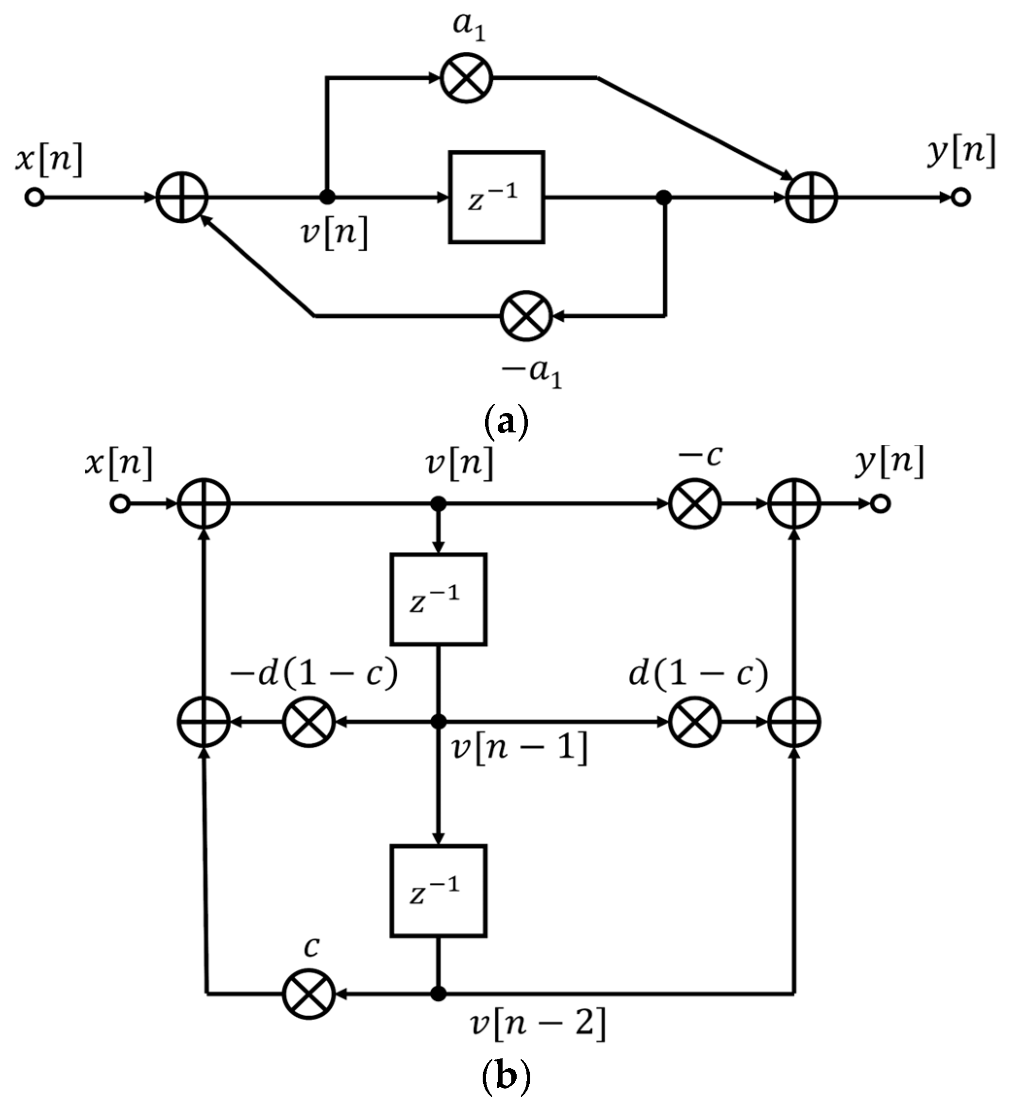
3.6. Numerical Solution for the Three-Stage Filter

As detailed above, the single-stage filter case around ϕ₀ =$-90°$ requires very small $Q$ values and very large $\xi$ values and central frequencies. This motivates us to utilise more stages. It turns out that a two-stage filter yields equivalent results to the single-stage filter: the numerically optimal two-stage filter is obtained when the two central frequencies coincide. If these central frequencies do not coincide, then one needs a third filter to ‘flatten out’ the phase shift. Motivated by this, we try to solve the three-stage filter case, where:

$$\varphi (\omega )={\varphi }_1(\omega )+{\varphi }_2(\omega )+{\varphi }_3(\omega )$$

(21)

Utilising the approximative formula of Equation (20) for each of the filters as follows

$${\varphi }_i(\omega )\approx 4·atan\left[{\displaystyle \frac{1}{2}}\left\{{{\xi }_i}^{-Q_i}-{{\xi }_i}^{Q_i}\right\}\right]+4Q_i^2{\displaystyle \frac{{{\xi }_i}^{Q_i}-{{\xi }_i}^{-Q_i}}{2+{{\xi }_i}^{2Q_i}+{{\xi }_i}^{-2Q_i}}}\cdot {(ln{\displaystyle \frac{\omega }{{\omega }_{0i}}})}^2$$

(22)

leaves us with the following nine parameters: $Q_1,Q_2,Q_3$, ${\xi }_{1 },{\xi }_{2 },{\xi }_3$ and ω_0,1, ω_0,2, ω_0,3. The central frequencies ω_0,A,i and ω_0,B,i can be calculated similarly to Equations (15) and (16).

Further investigation of the amplitude of $\varphi (\omega )$ defined in Equation (21) reveals that many of the parameters are highly correlated. To achieve a symmetric $\varphi (\omega )$ in the desired frequency range, it can be empirically found that the optimal choice (in terms of the simplicity of the formulas and symmetry of $\varphi (\omega )$) is to set the following constraints as follows:

$$Q_3=Q_1, {\xi }_3={\xi }_1, {\omega }_{0,2}={\omega }_{0,1}{\displaystyle \frac{{\xi }_2}{{\xi }_1}}, {\omega }_{0,3}={\omega }_{0,1}{{\xi }_2}^2.$$

This leaves us with five free parameters: $Q_1,Q_2, {\xi }_1, {\xi }_2,{\omega }_{0,1}$, which are still correlated. Further empirical investigation of the level of constantness of $\varphi (\omega )$ finds that three of these ($Q_1,{\xi }_2,{\omega }_{0,1}$) can be fixed to almost arbitrary values (i.e., these represent weak modes), as long as the remaining two ($Q_2,{\xi }_1$, representing strong modes) are set appropriately. These remaining two have to be set such that the desired $\varphi (\omega )\approx$ϕ₀ is reached. When the original formula of Equation (7) is utilised (not the above approximation of Equation (22)), the optimal choice of parameters is as follows (with $\varphi$ understood in radians):

$$Q_1=P_1, Q_2=P_2\cdot {\Phi }_0, {\omega }_{0,1}=O_1,$$

$${\xi }_1=1+X_1\cdot {\varphi }_0+X_2\cdot {\varphi }_0^2-X_3\cdot {\varphi }_0^3, {\xi }_2=X_4,$$

where:

$$P_1=0.873, P_2=-0.06661, O_1=10.668 Hz,$$

$$X_1=0.00063792, X_2=0.0023086, X_3=0.0066800, X_4=44.595$$

The original central frequencies can thus be calculated from these parameters based on Equations (15) and (16). Furthermore, we find that the best result can be achieved if a small residual correction is applied, i.e., for $Q_2$ and ${\xi }_1$, a slightly modified ϕ₀ value is substituted. This correction can be expressed (with ϕ₀ in radians) as:

$${\varphi }_0^{(corr)}=0.0054919\cdot {\varphi }_0^3-0.0030961\cdot {\varphi }_0^2+0.98601\cdot {\varphi }_0-0.00044568$$

(23)

With this choice, a relatively constant $\varphi (\omega )$ can be achieved for several ϕ₀ values, as illustrated in Figure 17. The absolute deviation from the desired ϕ₀ value is also shown in Figure 17. Clearly, deviations increase as ϕ₀ increases, but they are always below ${0.5}^{°}$. Most probably, the parameter values and functions can be numerically optimised further if required by the application.

Values for the parameters $Q_i,{\xi }_i,{\omega }_{0,i}$, as well as ω_0,A,i and ω_0,B,i, for several ϕ₀ choices are given in Appendix B. One may note here that ${\xi }_1$ (and with that ${\xi }_3$) is extremely close to 1 for $\left|{\varphi }_0\right|<{20}^{°}$. In fact, ${\xi }_1$ is even slightly lower than 1, but this is a numerical artefact. In fact, for these cases, it can be understood that ${\xi }_1={\xi }_3=1$. This also means that filters number 1 and 3 are effectively cancelled, and only filter number 2 remains in use. At this point, we can recall from the previous section that the single-stage filter was quite effective for smaller absolute values of ϕ₀. Here, it turns out that even with three filters, the above-described, partly intuitive numerical optimization does cancel two of them. They become important for $\left|{\varphi }_0\right|$ values above approximately ${20}^{°},$ and especially near ${90}^{°}$.

4. Discussion

We now have the optimal parameters for a single-stage and a three-stage filter as well, so it is adequate to investigate their performances in terms of the constancy of the phase shift. A comparison of the single-stage and three-stage filters for ϕ₀ = $-\pi /2$ is shown in Figure 18. Here, the single-stage filter parameters were calculated based on the previous section, with $Q=0.1$ and $Q=0.05,$ and the interpolator was used to find the correct value for $\xi$ (which is $\xi =61.31$ in the former case, $\xi =3312$ in the latter one) corresponding to ${\omega }_{0,B}$ of 33.6 kHz and 1.814 MHz, i.e., quite large values which are potentially unattainable in a digital implementation. On the other hand, for the three-stage filter, central frequencies are always <22 kHz. This underlines that, for ϕ₀ = $-\pi /2$, the three-stage filter provides a much better solution than the single-stage one.

The codes implementing the above are given in [19] and can be readily used to implement the optimised three-stage filter.

5. Conclusions

In this paper, we present a new, frequency-independent phase shift technique that reduces the number of stages needed, and instead, we introduce the Q-factor as a variable which can be adjusted accordingly for the desired outcome. The accuracy of the technique presented here is dependent on both the frequency and the desired phase shift, with both higher and lower frequencies giving less accurate results. We find a relatively simple analytical formula for the single-stage filter, for which the optimal parameters are found numerically for the range of desired phase shifts [0–90°]. However, for the single-stage filter to be adequately uniform, unfeasibly large central frequencies have to be utilised for phase shifts above approximately 20°. In order to overcome this, a three-stage filter is introduced, and its optimal parameters are provided. In this case, the central frequencies for each of the filters are always below 22 kHz, providing a feasible possibility to implement a frequency-independent phase shift. We find that the three-stage filter is the best choice and that the numerical solution is adequate.

References

1. Madihian, M.; Watanabe, K.; Yamamoto, T. A Frequency-Independent Phase Shifter. J. Phys. E Sci. Instrum. 1979, 12, 1031–1032. [Google Scholar] [CrossRef]
2. Jones, B.K.; Sharma, B.K.; Bidle, D.H. A Frequency-Independent Phase Shifter. J. Phys. E Sci. Instrum. 1980, 13, 1346–1347. [Google Scholar] [CrossRef]
3. Helfric, A. Phase Shifter Using Digital Techniques. Electr. Des. News 1987, 32, 289–290. [Google Scholar]
4. Mittal, M.; Jamuar, S.S. Programmable Frequency-Independent Switched-Capacitor Phase Shifter of Unity Gain. Meas. Sci. Technol. 1991, 2, 475–477. [Google Scholar] [CrossRef]
5. Cowan, B. A Versatile Phase Shifter for NMR Experiments and Other Applications. Meas. Sci. Technol. 1992, 3, 296–298. [Google Scholar] [CrossRef]
6. Jung, D.H.; Ha, I.J. Low-Cost Sensorless Control of Brushless DC Motors Using a Frequency-Independent Phase Shifter. IEEE Trans. Power Electron. 2000, 15, 744–752. [Google Scholar] [CrossRef]
7. Lobb, W.E. Acoustic Sound System for a Room. U.S. Patent 4,837,829, 6 June 1989. [Google Scholar]
8. Zurcher, F. Sound Acquisition Method and System, and Sound Acquisition and Reproduction Apparatus. U.S. Patent 5,524,059, 4 June 1996. [Google Scholar]
9. Elko, G.W.; Teutsch, H. Second-Order Adaptive Differential Microphone Array. J. Acoust. Soc. Am. 2004, 115, 14. [Google Scholar] [CrossRef]
10. Oomen, P.; De Klerk, L. Environmental Sound Loudspeaker. Netherlands, Amsterdam: Patent WO/2023/287291, 19 January 2023. [Google Scholar]
11. Sedra, A.S.; Smith, K.C. Microelectronic Circuits, 3rd ed.; Saunders College Publishing: Philadelphia, PA, USA, 1992. [Google Scholar]
12. Cherepov, S.V. Bridge for AC Measurement of Magnetic Susceptibility. Instrum. Exp. Tech. 1986, 25, 1226–1227. [Google Scholar]
13. Batrachenko, V.S.; Zarubina, T.V. Controllable Digital Phase Shifter. Instrum. Exp. Tech. 1978, 21, 1344–1345. [Google Scholar]
14. Maslov, N.V.; Prikhnenko, R.E. Digital Phase Shifter for a Precision Calibrator of Phase Shifts. Instrum. Exp. Tech. 1978, 21, 1346–1347. [Google Scholar]
15. Sankaran, P.; Jagadeesh Kumar, V.; Sudhakar Rao, K. Precision Frequency-Independent Variable-Phase Phase Shifter. Electron. Lett. 1995, 31, 154–155. [Google Scholar] [CrossRef]
16. Abuelma’atti, M.T.; Baroudi, U. A Programmable Phase Shifter for Sinusoidal Signals. Act. Passiv. Electron. Compon. 1998, 21, 107–112. [Google Scholar] [CrossRef]
17. Al-Absi, M.A. A Simple Low Cost Frequency-Independent Phase Shifter. Arab. J. Sci. Eng. 2009, 34, 145–152. [Google Scholar]
18. Bitar, M.A.; Gallo, A.; Volpe, F.A. Multi-Pole Multi-Zero Frequency-Independent Phase-Shifter. Rev. Sci. Instrum. 2012, 83, 114703. [Google Scholar] [CrossRef]
19. Csanád, M. Frequency Independent Phase Shifter. GitHub. 2023. Available online: https://github.com/theworksinstitute/fips (accessed on 25 May 2024).
Figure 1. Implementation of (a) a first-order and (b) a second-order all-pass filter.
Acoustics 06 00039 g001
Figure 2. Implementation of a frequency-independent phase shifter.
Acoustics 06 00039 g002
Figure 3. Digital implementation of a (a) first-order and (b) second-order all-pass filter, where x[n] is the input signal; y[n] is the output signal; v[n] is the difference equation; Z−1 is the signal in the complex domain; and a, c, and d are parameters that control the break frequency, bandwidth, and cutoff frequency.
Acoustics 06 00039 g003
Figure 4. An all-pass band-stop filter, where x is the input signal; y is the output signal; and fch and fcl are the higher and lower cutoff frequencies, respectively.
Acoustics 06 00039 g004
Figure 5. Phase shift as a function of frequency, with ω 0 = 500 Hz and Q = 0.5–2.0.
Acoustics 06 00039 g005
Figure 6. Phase shift as a function of frequency for two three-stage filters with two different sets of parameters.
Acoustics 06 00039 g006
Figure 7. Phase difference as a function of frequency for a filter with two three-stage filters. The function shown in this plot is the difference of the two functions shown in Figure 6.
Acoustics 06 00039 g007
Figure 8. Phase difference as a function of frequency with parameters optimised for ϕ0 = −π/2.
Acoustics 06 00039 g008
Figure 9. Phase difference as a function of frequency: the same as Figure 8, but optimised for ϕ 0 = −0.259.
Acoustics 06 00039 g009
Figure 10. Plots showing χ2 as (a) a function of ω0,A and ω0,B with Q = 0.09 and (b) a function of Q and ω0,B with ω0,A = 3.5 Hz. The deep blue ‘valleys’ on both plots represent the set of minima.
Acoustics 06 00039 g010
Figure 11. Plot showing Δ ϕ as a function of Q and ξ . The deep blue region contains the most optimal solutions.
Acoustics 06 00039 g011
Figure 12. Plot showing ϕ0 as a function of Q and ξ . Each of the lines corresponds to a given ϕ0, i.e., ϕ0 is constant along them.
Acoustics 06 00039 g012
Figure 13. Lines in this plot represent ξ ( Q ) functions solving Equation (20) in the case of a given ϕ0, expressed in degrees for clarity.
Acoustics 06 00039 g013
Figure 14. Relative amplitude Δ ϕ /ϕ0 as a function of Q for various ϕ0 values.
Acoustics 06 00039 g014
Figure 15. The ξ value required for ϕ ( ω ) = ϕ0 as a function of ϕ0 for four different Q values.
Acoustics 06 00039 g015
Figure 16. Phase difference as a function of frequency for three different Q values.
Acoustics 06 00039 g016
Figure 17. Left: Numerically optimised ϕ(ω) curves for ϕ0 values from − 9 ° to − 189 ° in 9 ° increments (shown in units of radian). Right: The absolute deviation (in degrees) from the desired ϕ0 value.
Acoustics 06 00039 g017
Figure 18. Comparison of the numerically optimised three-stage filter and two single-stage filters for Q = 0.1 and Q = 0.05.
Acoustics 06 00039 g018
Disclaimer/Publisher’s Note: The statements, opinions and data contained in all publications are solely those of the individual author(s) and contributor(s) and not of MDPI and/or the editor(s). MDPI and/or the editor(s) disclaim responsibility for any injury to people or property resulting from any ideas, methods, instructions or products referred to in the content.