Investigation of LASSO Regression Method as a Correction Measurements’ Factor for Low-Cost Air Quality Sensors

Abstract

Air quality is a subject of study, particularly in densely populated areas, as it has been shown to affect human health and the local ecosystem. In recent years, with the rapid development of technology, low-cost sensors have emerged, with many people interested in the quality of the air in their area turning to the procurement of such sensors as they are affordable. The reliability of measurements from low-cost sensors remains a question in the research community. In this paper, the determination of the correction factor of low-cost sensor measurements by applying the least absolute shrinkage and selection operator (LASSO) regression method is investigated. The results are promising, as following the application of the correction factor determined through LASSO regression the adjusted measurements exhibit a closer alignment with the reference measurements. This approach ensures that the measurements from low-cost sensors become more reliable and trustworthy.

1. Introduction

In large cities with numerous human activities and various types of machinery, such as vehicles, industrial equipment, and heating systems, air quality must be monitored, as all of the above release gaseous pollutants into the environment [1]. Air quality has a direct impact on the health of the population. According to the World Health Organization [2], the poor quality of the air can cause various illnesses and even death. At a global level, air quality is monitored by governmental organizations and research centers with air quality monitoring systems consisting of expensive equipment. The advancement of technology has led to the rapid growth of low-cost sensors [3], which are small in size and affordable [4]. In recent years, there has been an observed trend among citizens to monitor air quality in their residential and work areas. To fulfill air quality monitoring requirements, they often resort to acquiring low-cost sensors. The reliability and accuracy of measurements [5] from low-cost sensors, especially on such a critical issue as air quality, remains a research question and is a continuous subject of research and study by the scientific community.

Air quality sensors should be considered as a complement to formal air quality monitoring instruments and not as a replacement [6]. By incorporating low-cost air quality sensors alongside formal air quality measuring instruments, it becomes feasible to establish an extensive monitoring network in a large city. This enables thorough spatial coverage within an area [7,8,9].

The calibration of low-cost electrochemical gas quality sensors, as indicated in the literature, can be performed through two methods. The first involves a laboratory environment [10,11,12,13], where the sensor is exposed to a specific quantity of the target gas, and the calibration function is derived. The second method involves field installation [14,15,16,17], positioning them alongside reference instruments, and the calibration function is developed through the correlation of measurements.

In both cases, the objective in calibration [18] is to find a function F such that the measurement values from the low-cost sensors $x_t$ approximate the values of the reference instruments $y_t$ (Equation (1)).

$$y_t=F\left(x_t\right)$$

(1)

In addition to the calibration process of low-cost sensors, a large number of research works have been carried out on the optimization of measurements from them. The application of linear regression and multiple linear regression to measurements of low-cost air quality sensors have shown correction factors with satisfactory results on the optimized measurements. Regression is one of the basic methods of analysis, as it is based on data used due to their simplicity and high degree of scalability [19]. The research works [20,21] report the use of linear regression, multivariate linear regression, and an artificial neural network to calibrate a cluster of low-cost O₃, NO₂, NO CO, and CO₂ sensors. Experimental results show that the artificial neural network can mitigate the effect of cross-sensitivity. In another work [22], calibration on a large number (more than 100) of metal-oxide ozone sensors of air pollution was performed using multiple linear regression. The research group [23] proposes a method for the calibration of portable gas sensors for accurate measurement of O₃ and NO₂ by utilizing linear regression, least squares, and major axis linear regression. Ιn the research work [24], the method of correcting measurements according to the quantitative variation in low-cost sensor measurements using linear regression is proposed.

Non-linear regression methods have been applied to optimize measurements in low-cost gas quality sensors. The work [25] shows the application of linear regression, multiple linear regression, and nonlinear regression to microparticles sensors, where the results of both multiple linear regression and nonlinear regression were equally good. According to the literature, many research papers [21,22,26,27,28] focus on sensor signal processing using nonlinear machine-learning algorithms (such as random forest (RF), artificial neural networks (ANN), support vector machine (SVM) methods, and the Kalman filtering (KF) approach) for the calibration of low-cost air quality sensors. In addition, advanced machine-learning (ML) methods, such as neural networks, have been applied to improve measurements from low-cost sensors, which yield better optimization as they are able to solve complex problems due to their robust performance [29,30,31]. The calibration of a low-cost sensor, when achieved by colocation next to reference instruments, requires a long measurement period to extract an effective calibration equation. Research works report on both remote [32] and global [33] calibration approaches, as they promise to be scalable and robust to concept drift or even sensor drift (in the case of continuous remote calibration). In other research works [34,35,36], the application of machine learning by means of a non-linear least absolute shrinkage and selection operator (LASSO) regression method is presented, in which both primary measurements of low-cost sensors and measurements of relative humidity, temperature, barometric pressure, wind speed, etc., are applied as independent variables of the LASSO function.

This work focuses on the study of optimization of measurements from low-cost electrochemical sensors that are used to estimate Nitrogen Dioxide (NO₂) and Ozone (O₃) pollutants’ concentration. This work’s contribution centers on striking a balance between results and effort, minimizing computational burden, by the utilization of simplified mathematical methods and applications for achieving excellent results. The used sensors are the NO2-B43F model for NO₂ and the OX-B431 model for O₃ both manufactured by Alphasense. The innovation is in the application of the least absolute shrinkage and selection operator (LASSO) regression method [37] where the nonlinear equation involves only one independent variable, that of the measurements. This study aims to investigate whether the LASSO regression method can optimize the measured values with only one independent variable and the parameters of the LASSO equation. LASSO regression is an analysis method that modulates both variable selection and normalization in order to improve the prediction accuracy and interpretability of the resulting statistical model. In addition, specific methodology scaling was applied in the experiment. The object of the study was to apply the LASSO regression to measurements both of the time scaling (period of 10 weeks of measurements) and seasonality scale (measurements of different months (summer, winter)) in order to determine whether the corrected measurements are affected by seasonality. The results are satisfactory in that the sensor readings after application of the method show values close to the actual reference values.

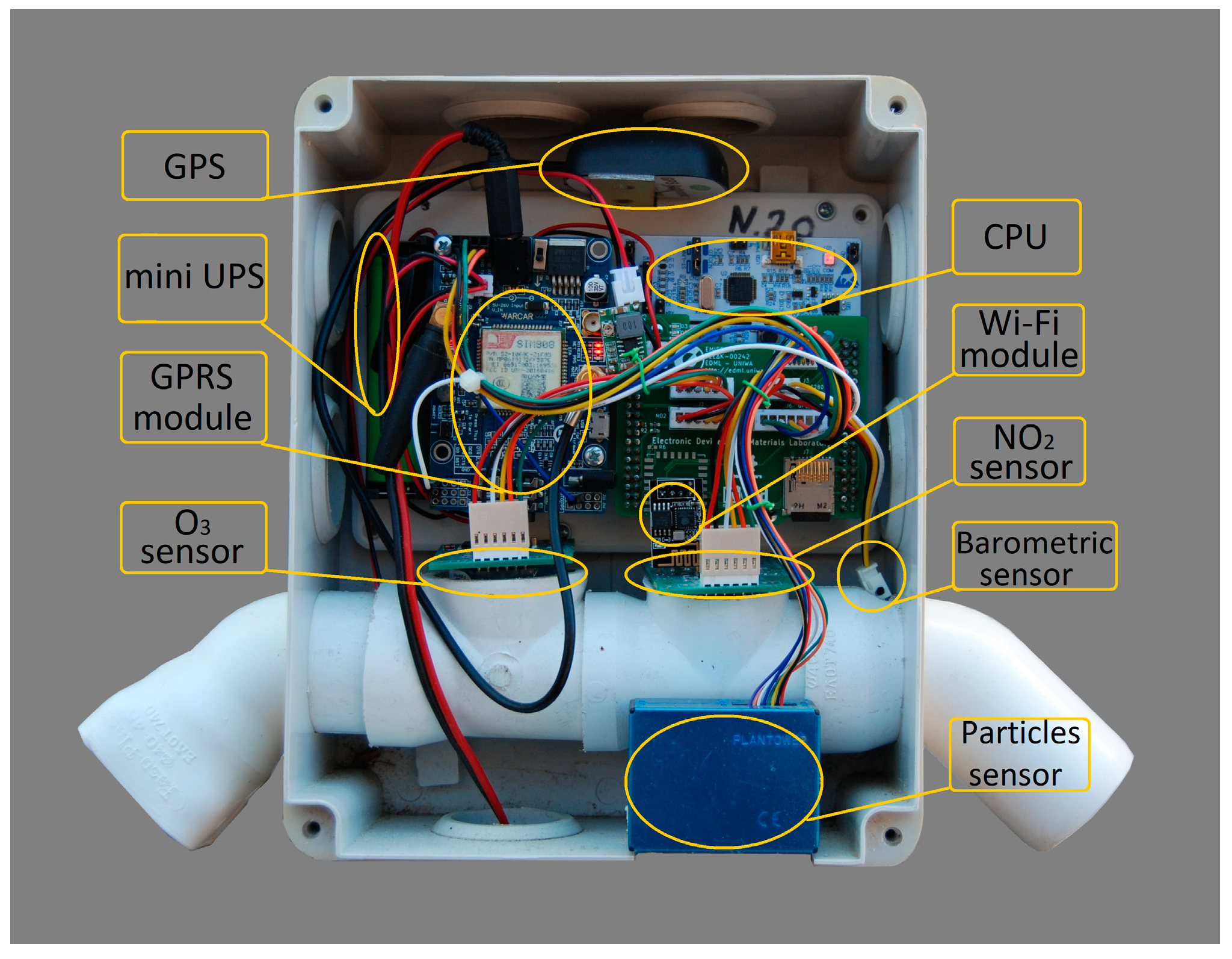
2. Low-Cost Monitoring Stations and Data Collection

Three low-cost gas monitoring stations [17] were developed in order to collect data. Initially, the three stations were installed next to official measuring points in order to perform initial calibration according to the manufacturer’s instructions, as will be described in this section. This procedure was run during February 2021. Sequentially, the monitoring stations were allowed to run on the field in parallel to the official stations and the collected data during the period 14 April–13 May were studied in the frame of this work. Details of the above described procedure follow below in Section 2 and Section 3. The low-cost stations are identified by a unique identifier (IDs 1, 2, 3). The study, design, and implementation of the gas-monitoring stations was carried out at the Electronic Devices and Materials Laboratory (EDML) of the department of Electrical and Electronics Engineering at the University of West Attica in Greece.

Each monitoring station (Figure 1) includes a microprocessor, gas pollutant sensors, peripheral auxiliary units, and a data transmission device (Wi-Fi, GPRS). The Nucleo STM-f091RC, STMicroelectronics, Schiphol, Netherlands, microprocessor, which offers a high processing speed and low power consumption, was used as the CPU, while electrochemical sensors, for NO₂ (NO2-B43F) and O₃ (OX-B431) manufactured by Alphasense [38], were used as gas pollutant sensors. In addition, an optical technology sensor was used for microparticle measurements: Plantower (PMS5003) [39]; while a barometric sensor (BME280) was used for barometric data acquisition. Finally, the auxiliary peripheral units are a GPS for installation location and data timing, a mini-UPS in case of occasional power loss, and a Wi-Fi or GPRS networking device for data transmission. Data are stored on an SD card in case of network transmission loss and sent when the connection is restored.

To ensure the reliability and reproducibility of the results, three identical low-cost air quality monitoring stations were installed in a densely populated neighborhood in the city center of Athens, at a height of 6–8 m above ground level, surrounded by main roads with heavy vehicular traffic. The measurements from the low-cost sensors were compared with the corresponding NO₂ and O₃ reference values obtained from the Ministry of Environment and Energy of Greece (PERPA) [40]. The reference scientific air quality monitoring station has been installed at the Ministry of Environment and Energy of Greece facilities in the center of Athens. Since both the locations of the low-cost air quality monitoring stations and the reference station are within the same area, they have the same air quality conditions. In particular, the installed air pollutant measurement devices are for O₃ the HORIBA APOA-360 automatic analyzer with ultraviolet absorption measurement method, and for NO₂ the HORIBA APNA-360 automatic analyzer with a chemiluminescence measurement method. The pollutants are measured continuously throughout the 24 h period. The response time of the automatic analyzers is one minute, while the hourly average pollution values are calculated hourly.

The operation of low-cost metering stations is carried out in accordance with the following sequence. Starting the station in operation, the timing signals, the analog ports, the digital input/output ports, and the communication buses with external devices (SPI, I2C, UART buses) are initialized on the CPU. During initialization, parameters such as node ID, measurement data, and GPS data are also determined. Then, the data structure packet is created for transmission, and finally the network connection (Wi-Fi or GPRS) is established. In the operation loop, measurements are taken every 10 s. In a 5 min period, the average of the measurements of each sensor together with the data from the GPS are structured into a transmission packet and sent to the server. If the acknowledgement of receipt of the packet is successful, a check is made to see if there are any records on the memory card that can be sent and then the operation stream is restarted. In case the acknowledgement of receipt of the packet fails, then the data are stored in the memory card and the loop starts again.

The electrochemical sensors used are from Alphasense [41] and use a four-electrode technology (working electrode, auxiliary electrode, counter electrode, reference electrode); the working electrode is exposed to ambient air as the oxidation or reduction of the gas to be measured takes place. The auxiliary electrode is an electrode with the same characteristics as the working electrode, which is placed in an electrolyte and therefore does not come into contact with the target gas. Because of its isolation from external conditions, it serves as a reference for the measurements of the working electrode. The counter electrode balances the reaction of the working electrode, where if the working electrode increases one molecule due to oxidation by the target gas, then the counter electrode must decrease another molecule to generate an equivalent current. The reference electrode operates according to the potential of the working electrode so that it always operates under the correct conditions. When the sensor is exposed to the target gas, the oxidation or reduction phenomenon occurs at the working electrode, which results in the creation of a current flowing from the working electrode to the opposite electrode or vice versa, depending on the phenomenon, with respect to the target gas. The generated current corresponds to the concentration of the target gas and can be used for calibration. An individual sensor board (ISB) circuit, as reported by Alphasense, provides both working electrode and auxiliary electrode measurements in mV. The conversion of the working and auxiliary electrode voltages to the target gas concentration is suggested by Alphasense’s Equation (2) [42] which includes the ambient temperature.

$${WE}_c=({WE}_u-{WE}_e)-n_T\ast ({AE}_u-{AE}_e)$$

(2)

where ${WE}_c$ represents the corrected value of the working electrode, ${WE}_u$ represents the measured value of the working electrode, ${AE}_u$ represents the measured value of the auxiliary electrode, $n_T$ represents the ambient temperature coefficient, ${WE}_e$ represents the electronic zero value of the working electrode, and $A{E}_e$ represents the electronic zero value of the auxiliary electrode. The values of ${WE}_e$ and ${AE}_e$ are given by the manufacturer for each sensor. The ${Gas}_{Measurement}$ concentration measurement is given by dividing the corrected output voltage ${WE}_c$ by ${Sensor}_{Sensitivity}$, as shown in Equation (3); the sensor sensitivity is also given for each sensor by the manufacturer.

$${Gas}_{Measurement}=\frac{{WE}_c}{{Sensor}_{Sensitivity}}$$

(3)

where ${Gas}_{Measurement}$ is the concentration measurement of the gas pollutant, ${WE}_c$ is the corrected working electrode value of the target gas given by Equation (2), and ${Sensor}_{Sensitivity}$ is given by the sensor manufacturer.

According to the manufacturer, a function must be applied when calibrating the sensors so that the corrected values of the measurements with this function are close to the reference values. Two correction factors [17] are calculated during the calibration period when colocating the low-cost monitoring station close to official instruments. The formula that yields the final corrected values by combining the two correction factors and the sensor measurements is shown in Equation (4):

$${GAS\_corrected}_{Measurement}=\left(\frac{({GAS}_{Measurement}+A)}{B}\right)$$

(4)

where ${GAS\_corrected}_{Measurement}$ is the calibrated gas sensor value, ${Gas}_{Measurement}$ is the corrected measurement concentration value of the gas pollutant by Equation (3), where A represents the level factor, which increases or decreases the measurement values to be corrected, and B represents the scaling factor, from which the corrected values of the measurement are derived. The last step of the procedure is the conversion of ppb to μg/m³. The initial calibration period was carried out in February 2021, at the field, by co-installing low-cost sensors next to a reference instrument. This process resulted in the determination of the A and B coefficients for each low-cost gas sensor. According to the manufacturer, to avoid incorrect gas measurements due to the cross-sensitivity of the Alphasense OX-B431 sensor, Equation (5) must be applied to the measurements in order to obtain the O₃ and NO₂ concentrations, since the O₃ electrochemical sensors are also triggered by NO₂,

$$O_{3}ppb=O_{3}All-{NO}_{2}ppb$$

(5)

where $O_{3}ppb$ is the ozone concentration measurement, ${NO}_{2}ppb$ is the NO₂ concentration value measured by the nitrogen dioxide sensor, and $O_{3}All$ is the concentration value measured by the ozone sensor.

3. Least Absolute Shrinkage and Selection Operator (LASSO) Regression

The study and the results of this paper are based on the LASSO method, offering a balance between simplicity and accuracy. LASSO is a linear regression technique to which a penalty term is added. The penalty term is proportional to the absolute value of the coefficients involved in the regression model equation, which means that some of the coefficients can be set to zero if they are considered less important. The size of the penalty is determined by the parameter λ. Τhe LASSO regression appears in Equation (6).

$$\sum _{i=1}^n(y_i-\sum _j{x_{ij}{\beta }_j)}^2+\lambda \sum _{j=1}^p\left|{\beta }_j\right|$$

(6)

The parameter λ controls the amount of the penalty. When λ takes the value of zero (0), all features are considered and the LASSO regression works like the simple standard linear regression. As λ increases, the penalty term becomes more significant, which results in the regression coefficients shrinking towards zero. The LASSO regression model is particularly useful in managing high-dimensional data, where the number of variables or characteristics is much larger than the number of observations. Traditional linear regression models suffer from overfitting when the model is too specific and complex, resulting in a poor performance on new, unseen data. LASSO regression can help to address this problem by identifying the most important variables and reducing the complexity of the model.

The implementation methodology was carried out according to the following steps.

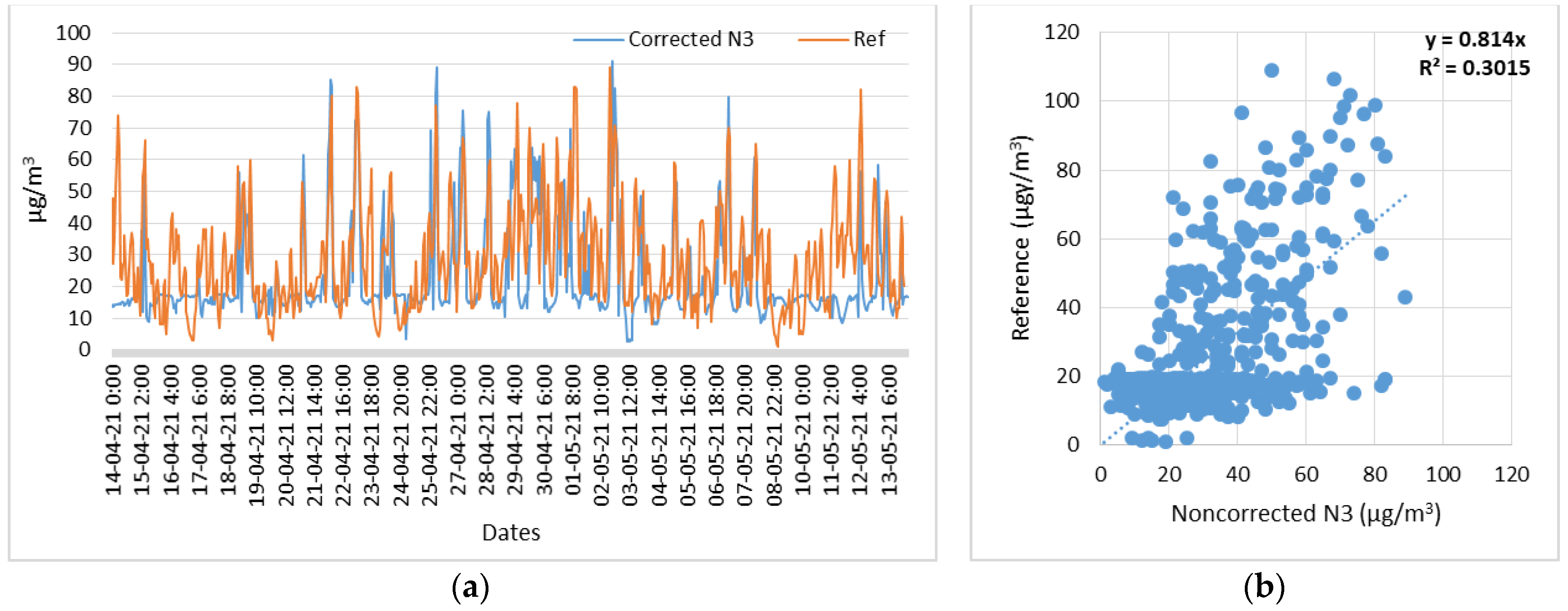
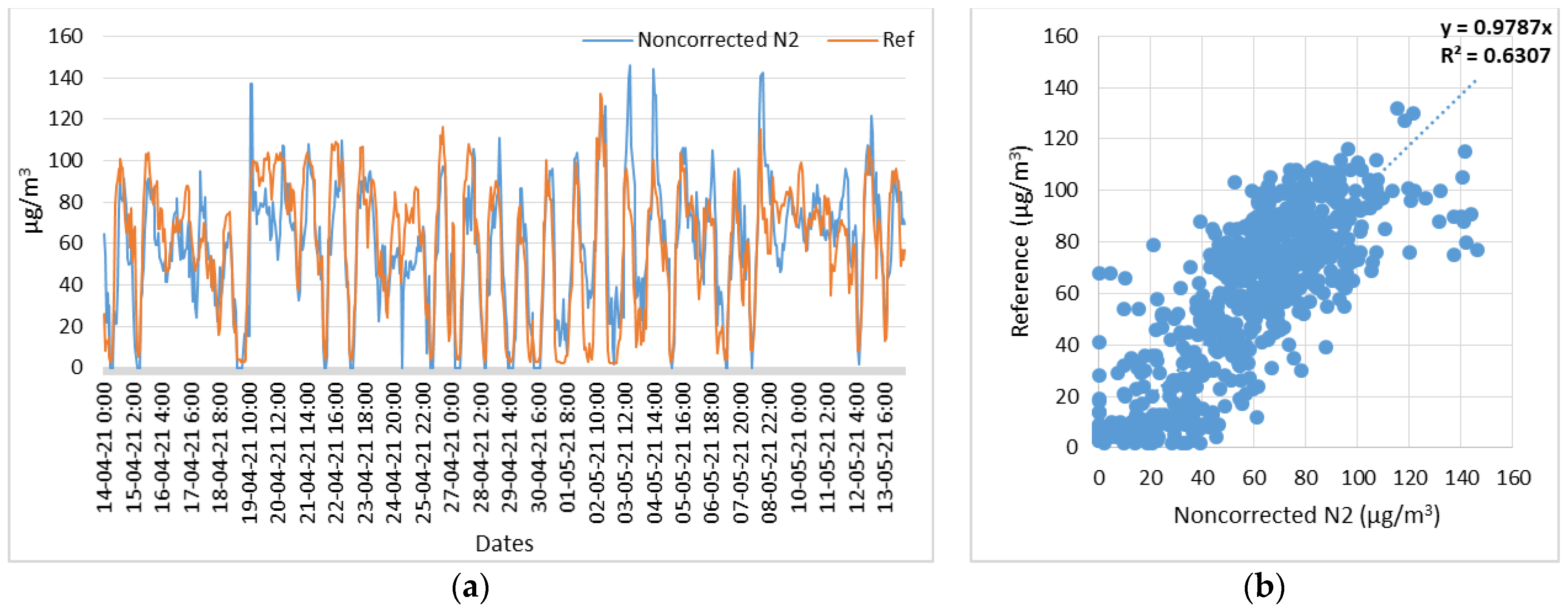
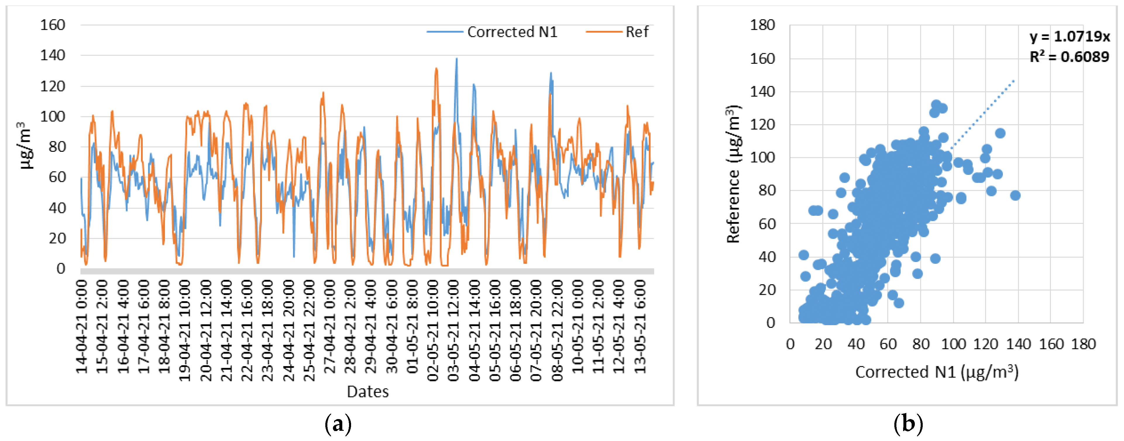
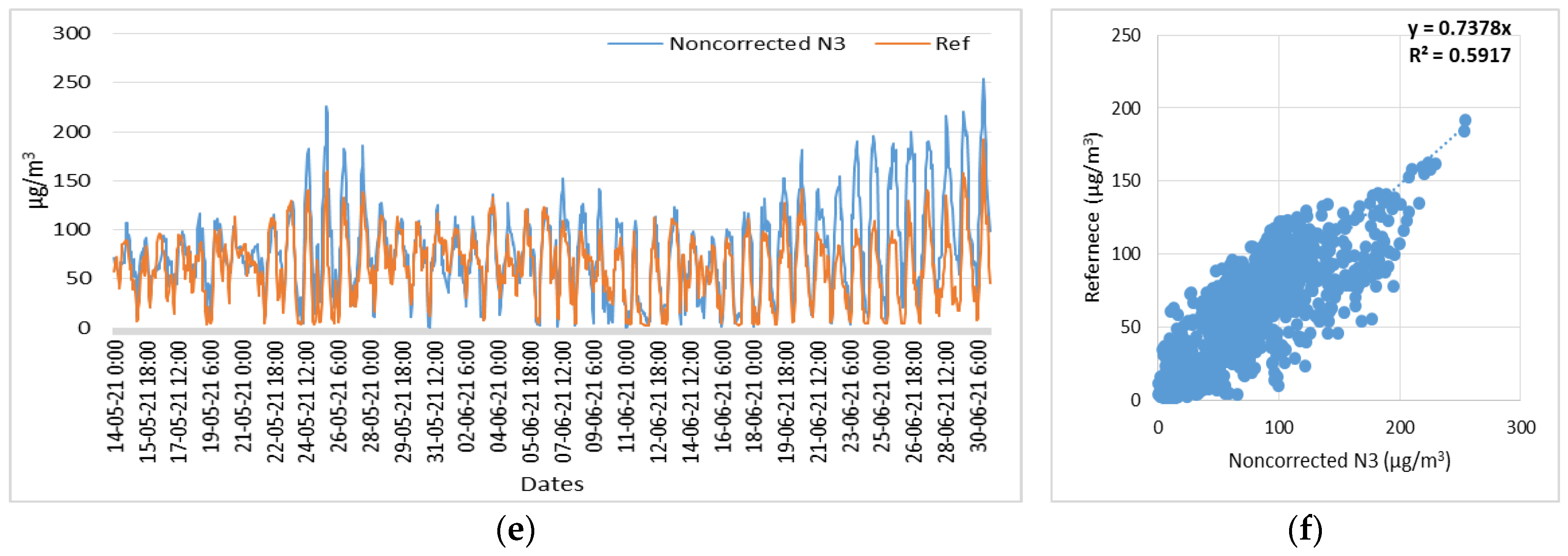
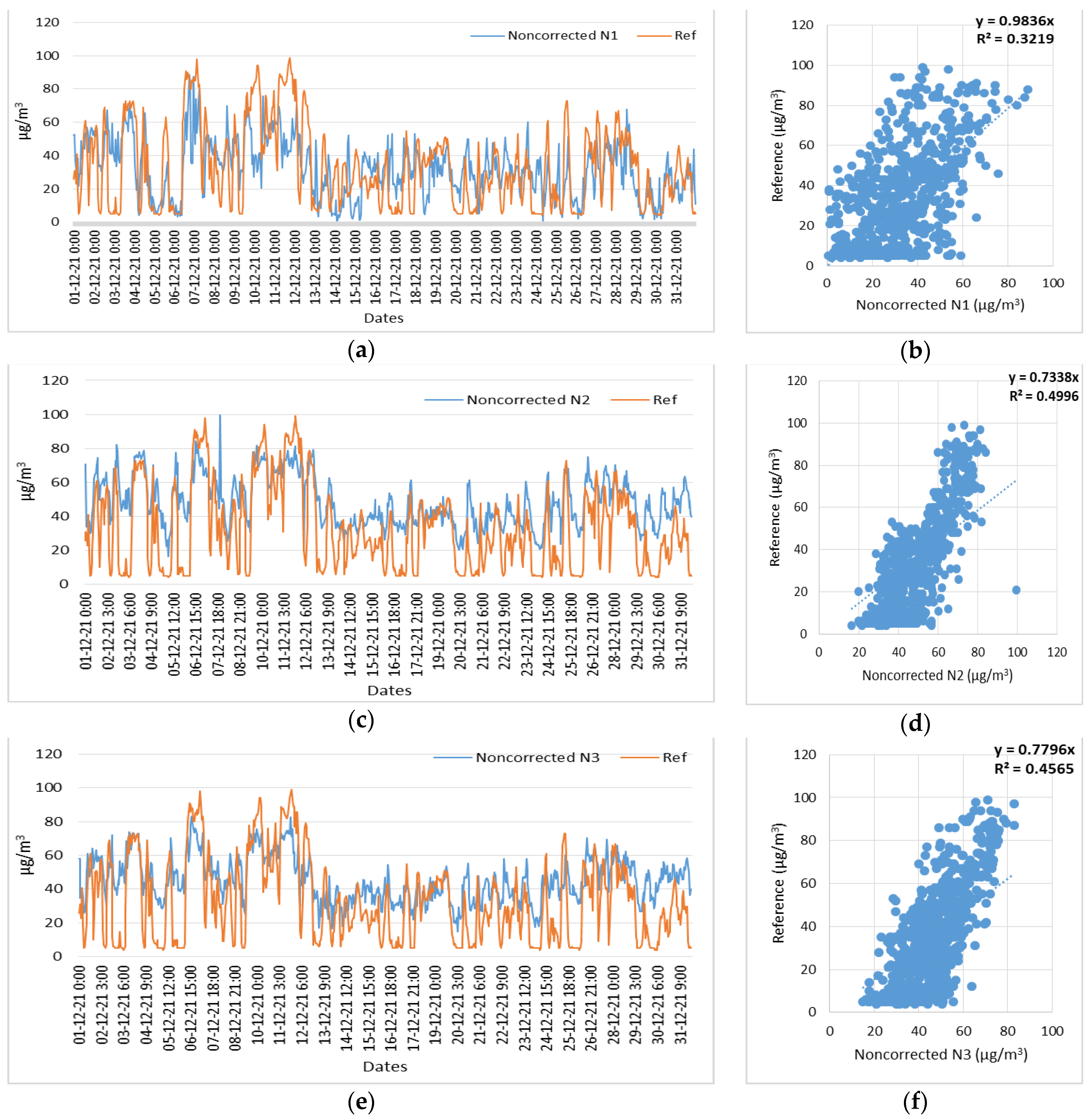
• First, the measurements collected by the pollutant sensors were correlated with the reference measurements. By this procedure, both the deviations of the measurements through the time series and the correlation coefficient between the measurements from the scatter plot were displayed;
• Τhe value of the parameter λ was estimated by means of the cross-validation deviance between the measurements of each low-cost sensor with the corresponding reference measurements. The λ parameter was calculated from the average of the λ parameter of all sensors of each gas, through the cross-validation deviation between the measurements of each low-cost sensor and the corresponding reference measurements;
• The estimated value of the parameter λ was applied according to the LASSO regression to the measurements of the low-cost sensors from which the corrected measurements were obtained by Equation (5);
• The corrected measurements were correlated with the reference measurements in order to identify the improvement of both the deviation of the measurements through the time series and the improvement of the correlation coefficient through the scatter plots.

Finally, for evaluation purposes, the methods MAD (mean absolute deviation), MAE (mean absolute error), and RMSE (root mean square error) were employed to assess the reliability and performance of the results across all datasets.

4. Results

The measurements of ΝO₂ and O₃ air pollutants are discussed below. Measurements at both the low-cost sensors (N1, N2, N3) and the reference sensors are conducted on an hourly basis. The data analysis implementation is performed in the MATLAB environment.

LASSO regression is utilized on the data to identify the divergence between measurements obtained from low-cost and reference sensors. This analysis aims to determine how this divergence can be corrected by adopting and adjusting the LASSO regression, turning it into a correction factor applicable to data from low-cost air quality sensors. This study referred to one month’s data (14 April 2021 to 13 May 2021), because the ageing of the sensors can impact the measurements [43]. For each low-cost sensor of both gases, ΝO₂ and O₃, the deviation λ and the coefficient B of the LASSO regression were identified. Then, using the simple linear equation (y = ax + b), the coefficients (a, b) of the equation were estimated according to the LASSO regression and applied to the measurements (x) from the low-cost sensors. The measurements from the gaseous pollutant sensors are henceforth referred to as noncorrected, whereas after the application of the LASSO regression they are henceforth referred to as corrected.

4.1. NO₂ Measurements

Regarding NO₂, the noncorrected sensor values are plotted against the reference values to identify the degree of correlation. Figure 2, Figure 3 and Figure 4 show both time series and scatter plots between the measurements from low-cost and reference sensors.

To determine the optimal value of the λ coefficient, cross-validation of the LASSO fit deviation, calculated for each sensor, between the low-cost sensor measurements and the reference ΝO₂ measurements was performed.

Figure 5a, Figure 6a, and Figure 7a show the NO₂ measurements’ cross-validated deviance diagram of each low-cost sensor (N1, N2, N3) and reference, respectively. Figure 5b, Figure 6b, and Figure 7b show the scatter plot between the NO₂ measurements of both the low-cost sensor (N1, N2, N3) and the reference. The scatter plot also shows the trend line for λ = 0 and for λ = 0.55.

Table 1. λ and B coefficients of LASSO regression of NO₂ low-cost sensors.

NO2 Sensors	λ	Β
N1	0.55	0.2463
N2	0.55	0.2885
N3	0.55	0.1905

shows the values of the λ and B coefficients of the LASSO regression for each low-cost NO₂ sensor.

From the extracted optimized trend line (for λ = 0.55), and according to the slope of the trend line, the coefficients of the simple linear equation y = ax + b were determined. Since the values start from the origin of the axes, b is equal to zero. The liner coefficient a was then estimated and applied to the measurements of each low-cost sensor of NO₂.

Figure 8a, Figure 9a, and Figure 10a show the corrected measurements of the NO₂ concentration of each sensor (N1, N2, N3) with respect to the reference measurements, respectively. Figure 8b, Figure 9b, and Figure 10b show the scatterplot of the NO₂ concentration between the corrected measurements of each sensor (N1, N2, N3) with respect to the reference measurements, respectively.

The aggregated results of the scatter plots of the low-cost NO₂ sensors before and after the application of the correction factors by means of the LASSO regression are shown in

Table 2. Linear coefficient and correlation degree (R²), before and after LASSO regression of NO₂ low-cost sensors’ measurements with respect to reference measurements.

NO2 Sensors	Before LASSO Regression		After LASSO Regression
	Linear Coefficient	R2	Linear Coefficient	R2
N1	0.8827	0.23	1.0396	0.27
N2	0.8598	0.22	0.9321	0.26
N3	0.9256	−0.028	1.081	0.05

.

4.2. O₃ Sensors

For O₃ (O₃), the noncorrected sensor values were plotted against the reference values to identify the degree of correlation. Figure 11, Figure 12 and Figure 13 show both time series and scatter plots between the measurements from low-cost and reference sensors.

To determine the optimal value of the λ coefficient, cross-validation of the LASSO fit deviation, calculated for each sensor, between the low-cost sensor measurements and the reference O₃ measurements was performed.

Figure 14a, Figure 15a, and Figure 16a show the O₃ measurements’ cross-validated deviance diagram of each low-cost sensor (N1, N2, N3) and reference, respectively. Figure 14b, Figure 15b, and Figure 16b show the scatter plot between the O₃ measurements of each low-cost sensor (N1, N2, N3) and reference. The scatter plot also shows the trend line for λ = 0 and for λ = 1.4.

Table 3. λ and B coefficients of LASSO regression of O₃ low-cost sensors.

O3 Sensors	λ	Β
N1	1.4	0.8763
N2	1.4	0.7873
N3	1.4	0.7852

shows the values of the λ and B coefficients of the LASSO regression for each low-cost O₃ sensor.

From the extracted optimized trend line (for λ = 1.4), and according to the slope of the trend line, the coefficients of the simple linear equation y = ax + b were determined. Since the values start from the origin of the axes, β is equal to zero. The coefficient a was then estimated and applied to the measurements of each low-cost sensor of O₃.

Figure 17a, Figure 18a, and Figure 19a show the corrected measurements of O₃ concentration of each sensor (N1, N2, N3) with respect to the reference measurements, respectively. Figure 17b, Figure 18b, and Figure 19b show the scatterplot of O₃ concentration between the corrected measurements of each sensor (N1, N2, N3) with respect to the reference measurements, respectively.

The aggregated results of the scatter plots of the low-cost O₃ sensors before and after the application of the correction factors by means of the LASSO regression are shown in

Table 4. Linear coefficient and correlation degree (R²), before and after LASSO regression of O₃ low-cost sensors’ measurements with respect to reference measurements.

O3 Sensors	Before LASSO Regression		After LASSO Regression
	Linear Coefficient	R2	Linear Coefficient	R2
N1	1.0385	0.60	1.0719	0.61
N2	0.9787	0.63	1.0007	0.65
N3	0.9067	0.57	0.9538	0.57

.

4.3. RMSE, MAD, and MAE Methods Evaluation

For the evaluation purpose of the results of LASSO regression method as a correction factor to measurements of low-cost air quality sensors, the methods of mean absolute deviation (MAD), mean absolute error (MAE), and root mean square error (RMSE), were applied to measurements data.

Table 5. MAD, MAE, and RMSE methods of evaluation of NO₂ measurements.

NO2
Method	MAD			MAE			RMSE
Sensors	N1	N2	N3	N1	N2	N3	N1	N2	N3
Non-corrected	2.29	3.47	2.57	11.78	12.89	10.16	0.90	1.04	1.45
Corrected	2.34	1.89	2.60	12.59	11.78	12.77	1.05	1.09	1.49

shows the RMSE, MAD, and MAE results of both noncorrected and corrected measurements for the three low-cost (N1, N2, N3) NO₂ sensors with respect to reference measurements.

Table 6. MAD, MAE, and RMSE methods of evaluation of O₃ measurements.

O3
Sensors	N1	N2	N3	N1	N2	N3	N1	N2	N3
Method	MAD			MAE			RMSE
Non-corrected	16.21	19.30	16.16	19.94	23.18	21.37	1.52	1.74	0.10
Corrected	13.78	15.98	14.92	17.03	19.59	20.05	1.54	1.69	0.13

shows the RMSE, MAD, and MAE results of both noncorrected and corrected measurements for the three low-cost (N1, N2, N3) O₃ sensors with respect to reference measurements.

4.4. Methodology Scaling

This section presents the results of scaling the proposed methodology. An extended study took place both for the time scaling and the seasonality scale. Data were processed in a bigger time frame and in different year seasons, with different environmental conditions.

4.5. Time Scaling

For the purpose of the evaluation of the time scaling of the experiment, the LASSO regression was also applied for a period of one and a half months after the one month of the main experiment (i.e., from 14 May 2021 to 31 June 2021) to all low-cost sensors, and the results are presented in the figures below. Figure 20 shows the time series and scatter plots of the NO₂ noncorrected measurements of three low-cost sensors (N1, N2, N3) and reference measurements, in the time period of 14 May 2021 to 31 June 2021. Figure 21 shows the time series and scatter plots of the NO₂ corrected measurements of three low-cost sensors (N1, N2, N3) and reference measurements, in the time period of 14 May 2021 to 31 June 2021.

Figure 22 shows the time series and scatter plots of the O₃ noncorrected measurements of three low-cost sensors (N1, N2, N3) and reference measurements, in the time period of 14 May 2021 to 31 June 2021. Figure 23 shows the time series and scatter plots of the O₃ corrected measurements of three low-cost sensors (N1, N2, N3) and reference measurements, in the time period of 14 May 2021 to 31 June 2021.

4.6. Seasonality Scale

In addition, in order to determine whether seasonality affects the results, the LASSO regression was applied during the winter month of December 2021 (i.e., from 1 December 2021 to 31 December 2021), to all low-cost sensors, and the results are shown in the figures below. Figure 24 shows the time series and scatter plots of the NO₂ noncorrected measurements of three low-cost sensors (N1, N2, N3) and reference measurements, in the time period of 1 December 2021 to 31 December 2021. Figure 25 shows the time series and scatter plots of the NO₂ corrected measurements of three low-cost sensors (N1, N2, N3) and reference measurements, in the time period of 1 December 2021 to 31 December 2021.

Figure 26 shows the time series and scatter plots of the O₃ noncorrected measurements of three low-cost sensors (N1, N2, N3) and reference measurements, in the time period of 1 December 2021 to 31 December 2021. Figure 27 shows the time series and scatter plots of the O₃ corrected measurements of three low-cost sensors (N1, N2, N3) and reference measurements, in the time period of 1 December 2021 to 31 December 2021.

5. Discussion

The application of the LASSO regression method for determining the correction factor to measurement data from low-cost air quality sensors, in particular electrochemical NO₂ and O₃ sensors, has been shown to improve the measurements from these sensors.

The experiment was carried out on one month’s data. For NO₂, the corrected measurements with the correction factor derived from the LASSO regression compared to the noncorrected measurements showed an improvement in the correlation coefficient (R²) of up to 4%, while the linear coefficient in the scatter plots of the corrected measurements in relation to the reference measurements shows a value closer to one (1). For O₃, the corrected values using LASSO regression showed that the degree of correlation (R²) could be improved by up to 2%, while the linear coefficient within the scatter plots of the corrected measurements in relation to the reference measurements also shows for these sensors a value closer to one (1) than for the noncorrected measurements. Although both remote and global calibration approaches promise scalability and robustness to deviation, the LASSO regression method shows satisfactory results with minimal computational power.

Although for both types of low-cost sensors, the correlation coefficient (R²) does not show a significant improvement, the linear coefficient contributes to the improvement of the measurements, as the corrected measurements are very close to the reference measurements, resulting in more realistic and trustworthy measurements. This observation occurs both for the time scaling in the month of the experiment (April 2021) and in the summer months (May, June 2021), as well as the seasonality scale between the summer months and the winter month (December 2021), which means that the correction with the LASSO regression method is not affected by time extension or seasonality.

To evaluate the correction factor using the LASSO regression method, the MAD, MAE, and RMSE methods were applied to both noncorrected and corrected measurements. Table 5 and Table 6 for NO₂ and O₃, respectively, show that, for NO₂, the values of the MAD, MAE and RMSE methods between corrected and noncorrected values show very small deviations which do not significantly affect the result. For O₃, the RMSE method showed very little divergence between the noncorrected and corrected measurements, while in the MAD and MAE methods the improvement is evident according to the results in Table 6. This correction achieved by the correction factor, which was identified by applying the LASSO regression, has the direct effect of improving the measurements to be closer to the real ones.

6. Conclusions

Air quality in large cities is an important issue as it can affect the health of citizens living in these areas. The development of technology has led to the rapid evolution of low-cost sensors. Inquiry into the trustworthiness and reliability of measurements obtained from low-cost sensors is a subject of research interest. Many research groups have presented, through their work, calibration and correction methods for low-cost sensor measurements to improve the reliability of measurements. In this work, the procedure for correcting measurements using the least absolute shrinkage and selection operator (LASSO) regression method from low-cost sensors, in particular from electrochemical NO₂ and O₃ sensors, is presented. In particular, the LASSO regression method was used in our experiment to identify a correction factor which was then applied to the measurements of the low-cost sensors to optimize the measurements from them.

The proposed methodology provides excellent results, as the results have shown that the correction factor identified using the LASSO regression contributes to the correction of measurements in low-cost electrochemical sensors. Although for both types of low-cost sensors (ΝO₂ and O₃) the improvement in the degree of correlation is not significant, the R² improvement for NO₂ of up to 4%, and the R² improvement for O₃ of up to 2%, it was observed that the linear correlation coefficient improves as it approaches the value of one (1). This resulted in the optimization of measurements from low-cost sensors, as the corrected measurements appear very close to the reference measurements. In addition, the methodology scaling shows excellent results, firstly at the time scaling of the total of two and a half months of corrected measurements by the LASSO regression method, and secondly at the seasonality scale of optimization of correction measurements by LASSO regression both of the summer and winter months. Implementing simplified mathematical processes in correcting the measurements, striking a balance between effort and results, proved to have an excellent performance. The methods MAD, MAE, and RMSE were applied to both uncorrected measurements and corrected measurements with the above mentioned method. The results showed negligible variation under the RMSE method, while for the MAD and MAE methods the corrected measurements show an improvement.

All field calibration methodologies have limitations arising from factors such as aging, the duration of the time period, specific environmental conditions, and seasonal variations. The proposed methodology can represent the core method of an adaptive methodology well using remotely available data and recalibration strategies. Extending this study could involve incorporating numerous cost-effective sensors, to provide a larger training data set, and conducting assessments at various locations exhibiting distinct atmospheric conditions.

The quality of air in the modern day needs to be monitored, and the use of low-cost sensors is becoming more and more widespread as many people are turning to the supply of such sensors because they are affordable. Measurements from low-cost sensors can be reliable and trustworthy by applying appropriate optimization models.

References

1. Gurjar, B.R.; Molina, L.T.; Ojha, C.S.P. Air Pollution: Health and Environmental Impacts; CRC Press: Boca Raton, FL, USA, 2010. [Google Scholar]
2. Ambient (Outdoor) Air Pollution. Available online: www.who.int.https://www.who.int/news-room/fact-sheets/detail/ambient-(outdoor)-air-quality-and-health/ (accessed on 16 December 2023).
3. Snyder, E.G.; Watkins, T.H.; Solomon, P.A.; Thoma, E.D.; Williams, R.W.; Hagler, G.S.W.; Shelow, D.; Hindin, D.A.; Kilaru, V.J.; Preuss, P.W. The Changing Paradigm of Air Pollution Monitoring. Environ. Sci. Technol. 2013, 47, 11369–11377. [Google Scholar] [CrossRef]
4. Jiao, W.; Hagler, G.; Williams, R.; Sharpe, R.; Brown, R.; Garver, D.; Judge, R.; Caudill, M.; Rickard, J.; Davis, M.; et al. Community Air Sensor Network (CAIRSENSE) Project: Evaluation of Low-Cost Sensor Performance in a Suburban Environment in the Southeastern United States. Atmos. Meas. Tech. 2016, 9, 5281–5292. [Google Scholar] [CrossRef]
5. Lewis, A.; Edwards, P. Validate Personal Air-Pollution Sensors. Nature 2016, 535, 29–31. [Google Scholar] [CrossRef]
6. Clements, A.L.; Griswold, W.G.; RS, A.; Johnston, J.E.; Herting, M.M.; Thorson, J.; Collier-Oxandale, A.; Hannigan, M. Low-Cost Air Quality Monitoring Tools: From Research to Practice (a Workshop Summary). Sensors 2017, 17, 2478. [Google Scholar] [CrossRef]
7. Rai, A.C.; Kumar, P.; Pilla, F.; Skouloudis, A.N.; Di Sabatino, S.; Ratti, C.; Yasar, A.; Rickerby, D. End-User Perspective of Low-Cost Sensors for Outdoor Air Pollution Monitoring. Sci. Total Environ. 2017, 607–608, 691–705. [Google Scholar] [CrossRef]
8. Ahangar, F.; Freedman, F.; Venkatram, A. Using Low-Cost Air Quality Sensor Networks to Improve the Spatial and Temporal Resolution of Concentration Maps. Int. J. Environ. Res. Public Health 2019, 16, 1252. [Google Scholar] [CrossRef]
9. Zheng, T.; Bergin, M.H.; Sutaria, R.; Tripathi, S.N.; Caldow, R.; Carlson, D.E. Gaussian Process Regression Model for Dynamically Calibrating and Surveilling a Wireless Low-Cost Particulate Matter Sensor Network in Delhi. Atmos. Meas. Tech. 2019, 12, 5161–5181. [Google Scholar] [CrossRef]
10. Heimann, I.; Bright, V.B.; McLeod, M.W.; Mead, M.I.; Popoola, O.A.M.; Stewart, G.B.; Jones, R.L. Source Attribution of Air Pollution by Spatial Scale Separation Using High Spatial Density Networks of Low Cost Air Quality Sensors. Atmos. Environ. 2015, 113, 10–19. [Google Scholar] [CrossRef]
11. Schneider, P.; Castell, N.; Vogt, M.; Dauge, F.R.; Lahoz, W.A.; Bartonova, A. Mapping Urban Air Quality in near Real-Time Using Observations from Low-Cost Sensors and Model Information. Environ. Int. 2017, 106, 234–247. [Google Scholar] [CrossRef]
12. Austin, C.C.; Roberge, B.; Goyer, N. Cross-Sensitivities of Electrochemical Detectors Used to Monitor Worker Exposures to Airborne Contaminants: False Positive Responses in the Absence of Target Analytes. J. Environ. Monit. 2006, 8, 161–166. [Google Scholar] [CrossRef]
13. Liu, D.; Zhang, Q.; Jiang, J.; Chen, D.-R. Performance Calibration of Low-Cost and Portable Particular Matter (PM) Sensors. J. Aerosol Sci. 2017, 112, 1–10. [Google Scholar] [CrossRef]
14. Motlagh, N.H.; Lagerspetz, E.; Nurmi, P.; Li, X.; Varjonen, S.; Mineraud, J.; Siekkinen, M.; Rebeiro-Hargrave, A.; Hussein, T.; Petaja, T.; et al. Toward Massive Scale Air Quality Monitoring. IEEE Commun. Mag. 2020, 58, 54–59. [Google Scholar] [CrossRef]
15. Borrego, C.; Costa, A.M.; Ginja, J.; Amorim, M.; Coutinho, M.; Karatzas, K.; Sioumis, T.; Katsifarakis, N.; Konstantinidis, K.; De Vito, S.; et al. Assessment of Air Quality Microsensors versus Reference Methods: The EuNetAir Joint Exercise. Atmos. Environ. 2016, 147, 246–263. [Google Scholar] [CrossRef]
16. Han, P.; Mei, H.; Liu, D.; Zeng, N.; Tang, X.; Wang, Y.; Pan, Y. Calibrations of Low-Cost Air Pollution Monitoring Sensors for CO, NO2, O3, and SO2. Sensors 2021, 21, 256. [Google Scholar] [CrossRef] [PubMed]
17. Christakis, I.; Hloupis, G.; Stavrakas, I.; Tsakiridis, O. Low Cost Sensor Implementation and Evaluation for Measuring NO2 and O3 Pollutants. In Proceedings of the 2020 9th International Conference on Modern Circuits and Systems Technologies (MOCAST), Bremen, Germany, 7–9 September 2020. [Google Scholar] [CrossRef]
18. Yu, H.; Li, Q.; Wang, R.; Chen, Z.; Zhang, Y.; Geng, Y.; Zhang, L.; Cui, H.; Zhang, K. A Deep Calibration Method for Low-Cost Air Monitoring Sensors with Multilevel Sequence Modeling. IEEE Trans. Instrum. Meas. 2020, 69, 7167–7179. [Google Scholar] [CrossRef]
19. Liang, L. Calibrating Low-Cost Sensors for Ambient Air Monitoring: Techniques, Trends, and Challenges. Environ. Res. 2021, 197, 111163. [Google Scholar] [CrossRef]
20. Spinelle, L.; Gerboles, M.; Villani, M.G.; Aleixandre, M.; Bonavitacola, F. Field Calibration of a Cluster of Low-Cost Available Sensors for Air Quality Monitoring. Part A: Ozone and Nitrogen Dioxide. Sens. Actuators B Chem. 2015, 215, 249–257. [Google Scholar] [CrossRef]
21. Spinelle, L.; Gerboles, M.; Villani, M.G.; Aleixandre, M.; Bonavitacola, F. Field Calibration of a Cluster of Low-Cost Commercially Available Sensors for Air Quality Monitoring. Part B: NO, CO and CO2. Sens. Actuators B Chem. 2017, 238, 706–715. [Google Scholar] [CrossRef]
22. Barceló-Ordinas, J.M.; García-Vidal, J.; Doudou, M.; Rodrigo, S.; Cerezo-Llavero, A. Calibrating Low-Cost Air Quality Sensors Using Multiple Arrays of Sensors. In Proceedings of the 2018 IEEE Wireless Communications and Networking Conference (WCNC), Barcelona, Spain, 15–18 April 2018. [Google Scholar] [CrossRef]
23. Lin, C.; Gillespie, J.; Schuder, M.D.; Duberstein, W.; Beverland, I.J.; Heal, M.R. Evaluation and Calibration of Aeroqual Series 500 Portable Gas Sensors for Accurate Measurement of Ambient Ozone and Nitrogen Dioxide. Atmos. Environ. 2015, 100, 111–116. [Google Scholar] [CrossRef]
24. Christakis, I.; Sarri, E.; Tsakiridis, O.; Stavrakas, I. Identification of the Safe Variation Limits for the Optimization of the Measurements in Low-Cost Electrochemical Air Quality Sensors. Electrochem 2023, 5, 1–28. [Google Scholar] [CrossRef]
25. Hong, G.-H.; Le, T.-C.; Tu, J.-W.; Wang, C.; Chang, S.-C.; Yu, J.-Y.; Lin, G.-Y.; Aggarwal, S.G.; Tsai, C.-J. Long-Term Evaluation and Calibration of Three Types of Low-Cost PM2.5 Sensors at Different Air Quality Monitoring Stations. J. Aerosol Sci. 2021, 157, 105829. [Google Scholar] [CrossRef]
26. De Vito, S.; Esposito, E.; Salvato, M.; Popoola, O.; Formisano, F.; Jones, R.; Di Francia, G. Calibrating Chemical Multisensory Devices for Real World Applications: An In-Depth Comparison of Quantitative Machine Learning Approaches. Sens. Actuators B Chem. 2018, 255, 1191–1210. [Google Scholar] [CrossRef]
27. Bigi, A.; Mueller, M.; Grange, S.K.; Ghermandi, G.; Hueglin, C. Performance of NO, NO2 Low Cost Sensors and Three Calibration Approaches within a Real World Application. Atmos. Meas. Tech. 2018, 11, 3717–3735. [Google Scholar] [CrossRef]
28. Christakis, I.; Tsakiridis, O.; Kandris, D.; Stavrakas, I. A Kalman Filter Scheme for the Optimization of Low-Cost Gas Sensor Measurements. Electronics 2024, 13, 25. [Google Scholar] [CrossRef]
29. Giordano, M.R.; Malings, C.; Pandis, S.N.; Presto, A.A.; McNeill, V.F.; Westervelt, D.M.; Beekmann, M.; Subramanian, R. From Low-Cost Sensors to High-Quality Data: A Summary of Challenges and Best Practices for Effectively Calibrating Low-Cost Particulate Matter Mass Sensors. J. Aerosol Sci. 2021, 158, 105833. [Google Scholar] [CrossRef]
30. Mahajan, S.; Kumar, P. Evaluation of Low-Cost Sensors for Quantitative Personal Exposure Monitoring. Sustain. Cities Soc. 2020, 57, 102076. [Google Scholar] [CrossRef]
31. Zimmerman, N.; Presto, A.A.; Kumar, S.P.N.; Gu, J.; Hauryliuk, A.; Robinson, E.S.; Robinson, A.L. A Machine Learning Calibration Model Using Random Forests to Improve Sensor Performance for Lower-Cost Air Quality Monitoring. Atmos. Meas. Tech. 2018, 11, 291–313. [Google Scholar] [CrossRef]
32. Miskell, G.; Alberti, K.; Feenstra, B.; Henshaw, G.S.; Papapostolou, V.; Patel, H.; Polidori, A.; Salmond, J.A.; Weissert, L.; Williams, D.E. Reliable Data from Low Cost Ozone Sensors in a Hierarchical Network. Atmos. Environ. 2019, 214, 116870. [Google Scholar] [CrossRef]
33. De Vito, S.; D’Elia, G.; Ferlito, S.; Di Francia, G.; Davidović, M.D.; Kleut, D.; Stojanović, D.; Jovaševic-Stojanović, M. A Global Multi-Unit Calibration as a Method for Large Scale IoT Particulate Matter Monitoring Systems Deployments. IEEE Trans. Instrum. Meas. 2024, 73, 1–16. [Google Scholar] [CrossRef]
34. Sethi, J.K.; Mittal, M. An Efficient Correlation Based Adaptive LASSO Regression Method for Air Quality Index Prediction. Earth Sci. Inform. 2021, 14, 1777–1786. [Google Scholar] [CrossRef]
35. Liu, B.; Jin, Y.; Xu, D.; Wang, Y.; Li, C. A Data Calibration Method for Micro Air Quality Detectors Based on a LASSO Regression and NARX Neural Network Combined Model. Sci. Rep. 2021, 11, 21173. [Google Scholar] [CrossRef]
36. Sahu, R.; Nagal, A.; Dixit, K.K.; Unnibhavi, H.; Mantravadi, S.; Nair, S.; Simmhan, Y.; Mishra, B.; Zele, R.; Sutaria, R.; et al. Robust Statistical Calibration and Characterization of Portable Low-Cost Air Quality Monitoring Sensors to Quantify Real-Time O3 and NO2 Concentrations in Diverse Environments. Atmos. Meas. Tech. 2021, 14, 37–52. [Google Scholar] [CrossRef]
37. Tibshirani, R. Regression Shrinkage and Selection via the Lasso. J. R. Stat. Soc. Ser. B (Methodol.) 1996, 58, 267–288. [Google Scholar] [CrossRef]
38. Alphasense UK—Browse Gas Sensors & Air Quality Monitors. Alphasense. Available online: http://www.alphasense.com (accessed on 14 December 2023).
39. PMS5003—Laser PM2.5 Sensor-Plantower Technology. Available online: https://www.plantower.com/en/products_33/74.html (accessed on 14 December 2023).
40. Air Pollution Measurement Data. Ministry of Environment & Energy, Greece. Available online: https://ypen.gov.gr/perivallon/poiotita-tis-atmosfairas/dedomena-metriseon-atmosfairikis-rypansis/ (accessed on 14 December 2023).
41. AAN. Alphasense Application Note AAN 104 How Electrochemical Gas Sensors Work. Available online: https://www.alphasense.com/wp-content/uploads/2013/07/AAN_104.pdf (accessed on 14 December 2023).
42. Alphasense. Alphasense Application Note AAN 803-01 Correcting for Background Currents in Four Electrode Toxic Gas Sensors; Alphasense: Braintree, UK, 2014; Available online: https://zueriluft.ch/makezurich/AAN803.pdf (accessed on 14 December 2023).
43. Christakis, I.; Tsakiridis, O.; Kandris, D.; Stavrakas, I. Air Pollution Monitoring via Wireless Sensor Networks: The Investigation and Correction of the Aging Behavior of Electrochemical Gaseous Pollutant Sensors. Electronics 2023, 12, 1842. [Google Scholar] [CrossRef]
Figure 1. Low-cost gas and particle matter monitoring station.
Signals 05 00004 g001
Figure 2. Node 1, NO2 noncorrected measurements with respect to reference measurements. (a) Time series of N1 (NO2) noncorrected and reference measurements; (b) Scatterplot of N1 (NO2) noncorrected and reference measurements.
Signals 05 00004 g002
Figure 3. Node 2, NO2 noncorrected measurements with respect to reference measurements. (a) Time series of N2 (NO2) noncorrected and reference measurements; (b) Scatterplot of N2 (NO2) noncorrected and reference measurements.
Signals 05 00004 g003
Figure 4. Node 3, NO2 noncorrected measurements with respect to reference measurements. (a) Time series of N3 (NO2) noncorrected and reference measurements; (b) Scatterplot of N3 (NO2) noncorrected and reference measurements.
Signals 05 00004 g004
Figure 5. NO2 N1, cross-validated deviance diagram and scatter plot with different values of λ. (a) The cross-validated deviance diagram of NO2 measurements between low-cost N1 and reference sensors; (b) Scatter plot of NO2 measurements between low-cost N1 and reference for λ = 0 and λ = 0.55.
Signals 05 00004 g005
Figure 6. NO2 N2, cross-validated deviance diagram and scatter plot with different values of λ. (a) The cross-validated deviance diagram of NO2 measurements between low-cost N2 and reference sensors; (b) Scatter plot of NO2 measurements between low-cost N2 and reference for λ = 0 and λ = 0.55.
Signals 05 00004 g006
Figure 7. NO2 N3, cross-validated deviance diagram and scatter plot with different values of λ. (a) The cross-validated deviance diagram of NO2 measurements between low-cost N3 and reference sensors; (b) Scatter plot of NO2 measurements between low-cost N3 and reference for λ = 0 and λ = 0.55.
Signals 05 00004 g007
Figure 8. Node 1, NO2 corrected measurements with respect to reference measurements. (a) Time series of N1 (NO2) corrected and reference measurements; (b) Scatterplot of N1 (NO2) corrected and reference measurements.
Signals 05 00004 g008
Figure 9. Node 2, NO2 corrected measurements with respect to reference measurements. (a) Time series of N2 (NO2) corrected and reference measurements; (b) Scatterplot of N2 (NO2) corrected and reference measurements.
Signals 05 00004 g009
Figure 10. Node 3, NO2 corrected measurements with respect to reference measurements. (a) Time series of N3 (NO2) corrected and reference measurements; (b) Scatterplot of N3 (NO2) corrected and reference measurements.
Signals 05 00004 g010
Figure 11. Node 1, O3 noncorrected measurements with respect to reference measurements. (a) Time series of N1 (O3) noncorrected and reference measurements; (b) Scatterplot of N1 (O3) noncorrected and reference measurements.
Signals 05 00004 g011
Figure 12. Node 2, O3 noncorrected measurements with respect to reference measurements. (a) Time series of N2 (O3) noncorrected and reference measurements; (b) Scatterplot of N2 (O3) noncorrected and reference measurements.
Signals 05 00004 g012
Figure 13. Node 3, O3 noncorrected measurements with respect to reference measurements. (a) Time series of N3 (O3) noncorrected and reference measurements; (b) Scatterplot of N3 (O3) noncorrected and reference measurements.
Signals 05 00004 g013
Figure 14. O3 N1, cross-validated deviance diagram and scatter plot with different values of λ. (a) The cross-validated deviance diagram of O3 measurements between low-cost N1 and reference sensors; (b) Scatter plot of O3 measurements between low-cost N1 and reference for λ = 0 and λ = 1.4.
Signals 05 00004 g014
Figure 15. O3 N2, cross-validated deviance diagram and scatter plot with different values of λ. (a) The cross-validated deviance diagram of O3 measurements between low-cost N2 and reference sensors; (b) Scatter plot of O3 measurements between low-cost N2 and reference for λ = 0 and λ = 1.4.
Signals 05 00004 g015
Figure 16. O3 N3, cross-validated deviance diagram and scatter plot with different values of λ. (a) The cross-validated deviance diagram of O3 measurements between low-cost N3 and reference sensors; (b) Scatter plot of O3 measurements between low-cost N3 and reference for λ = 0 and λ = 1.4.
Signals 05 00004 g016
Figure 17. Node 1, O3 corrected measurements with respect to reference measurements. (a) Time series of N1 (O3) corrected and reference measurements; (b) Scatterplot of N1 (O3) corrected and reference measurements.
Signals 05 00004 g017
Figure 18. Node 2, O3 corrected measurements with respect to reference measurements. (a) Time series of N2 (O3) corrected and reference measurements; (b) Scatterplot of N2 (O3) corrected and reference measurements.
Signals 05 00004 g018
Figure 19. Node 3, O3 corrected measurements with respect to reference measurements. (a) Time series of N3 (O3) corrected and reference measurements; (b) Scatterplot of N3 (O3) corrected and reference measurements.
Signals 05 00004 g019
Figure 20. Time series and scatter plots of the NO2 noncorrected measurements of three low-cost sensors (N1, N2, N3) and reference measurements, in the time period of 14 May 2021 to 31 June 2021. (a) Time series of N1 (NO2) noncorrected and reference measurements; (b) Scatterplot of N1 (NO2) noncorrected and reference measurements; (c) Time series of N2 (NO2) noncorrected and reference measurements; (d) Scatterplot of N2 (NO2) noncorrected and reference measurements; (e) Time series of N3 (NO2) noncorrected and reference measurements; (f) Scatterplot of N3 (NO2) noncorrected and reference measurements.
Signals 05 00004 g020aSignals 05 00004 g020b
Figure 21. Time series and scatter plots of the NO2 corrected measurements of three low-cost sensors (N1, N2, N3) and reference measurements, in the time period of 14 May 2021 to 31 June 2021. (a) Time series of N1 (NO2) corrected and reference measurements; (b) Scatterplot of N1 (NO2) corrected and reference measurements; (c) Time series of N2 (NO2) corrected and reference measurements; (d) Scatterplot of N2 (NO2) corrected and reference measurements; (e) Time series of N3 (NO2) corrected and reference measurements; (f) Scatterplot of N3 (NO2) corrected and reference measurements.
Signals 05 00004 g021aSignals 05 00004 g021b
Figure 22. Time series and scatter plots of the O3 noncorrected measurements of three low-cost sensors (N1, N2, N3) and reference measurements, in the time period of 14 May 2021 to 31 June 2021. (a) Time series of N1 (O3) noncorrected and reference measurements; (b) Scatterplot of N1 (O3) noncorrected and reference measurements; (c) Time series of N2 (O3) noncorrected and reference measurements; (d) Scatterplot of N2 (O3) noncorrected and reference measurements; (e) Time series of N3 (O3) noncorrected and reference measurements; (f) Scatterplot of N3 (O3) noncorrected and reference measurements.
Signals 05 00004 g022aSignals 05 00004 g022b
Figure 23. Time series and scatter plots of the O3 corrected measurements of three low-cost sensors (N1, N2, N3) and reference measurements, in the time period of 14 May 2021 to 31 June 2021. (a) Time series of N1 (O3) corrected and reference measurements; (b) Scatterplot of N1 (O3) corrected and reference measurements; (c) Time series of N2 (O3) corrected and reference measurements; (d) Scatterplot of N2 (O3) corrected and reference measurements; (e) Time series of N3 (O3) corrected and reference measurements; (f) Scatterplot of N3 (O3) corrected and reference measurements.
Signals 05 00004 g023aSignals 05 00004 g023b
Figure 24. Time series and scatter plots of the NO2 noncorrected measurements of three low-cost sensors (N1, N2, N3) and reference measurements, in the time period of 1 December 2021 to 31 December 2021. (a) Time series of N1 (NO2) noncorrected and reference measurements; (b) Scatterplot of N1 (NO2) noncorrected and reference measurements; (c) Time series of N2 (NO2) noncorrected and reference measurements; (d) Scatterplot of N2 (NO2) noncorrected and reference measurements; (e) Time series of N3 (NO2) noncorrected and reference measurements; (f) Scatterplot of N3 (NO2) noncorrected and reference measurements.
Signals 05 00004 g024aSignals 05 00004 g024b
Figure 25. Time series and scatter plots of the NO2 corrected measurements of three low-costs sensors (N1, N2, N3) and reference measurements, in the time period of 1 December 2021 to 31 December 2021. (a) Time series of N1 (NO2) corrected and reference measurements; (b) Scatterplot of N1 (NO2) corrected and reference measurements; (c) Time series of N2 (NO2) corrected and reference measurements; (d) Scatterplot of N2 (NO2) corrected and reference measurements; (e) Time series of N3 (NO2) corrected and reference measurements; (f) Scatterplot of N3 (NO2) corrected and reference measurements.
Signals 05 00004 g025
Figure 26. Time series and scatter plots of the O3 noncorrected measurements of three low-cost sensors (N1, N2, N3) and reference measurements, in the time period of 1 December 2021 to 31 December 2021. (a) Time series of N1 (O3) noncorrected and reference measurements; (b) Scatterplot of N1 (O3) noncorrected and reference measurements; (c) Time series of N2 (O3) noncorrected and reference measurements; (d) Scatterplot of N2 (O3) noncorrected and reference measurements; (e) Time series of N3 (O3) noncorrected and reference measurements; (f) Scatterplot of N3 (O3) noncorrected and reference measurements.
Signals 05 00004 g026
Figure 27. Time series and scatter plots of the O3 corrected measurements of three low-cost sensors (N1, N2, N3) and reference measurements, in the time period of 1 December 2021 to 31 December 2021. (a) Time series of N1 (O3) corrected and reference measurements; (b) Scatterplot of N1 (O3) corrected and reference measurements; (c) Time series of N2 (O3) corrected and reference measurements; (d) Scatterplot of N2 (O3) corrected and reference measurements; (e) Time series of N3 (O3) corrected and reference measurements; (f) Scatterplot of N3 (O3) corrected and reference measurements.
Signals 05 00004 g027