Object Detection with Hyperparameter and Image Enhancement Optimisation for a Smart and Lean Pick-and-Place Solution

Abstract

Pick-and-place operations are an integral part of robotic automation and smart manufacturing. By utilizing deep learning techniques on resource-constraint embedded devices, the pick-and-place operations can be made more accurate, efficient, and sustainable, compared to the high-powered computer solution. In this study, we propose a new technique for object detection on an embedded system using SSD Mobilenet V2 FPN Lite with the optimisation of the hyperparameter and image enhancement. By increasing the Red Green Blue (RGB) saturation level of the images, we gain a 7% increase in mean Average Precision (mAP) when compared to the control group and a 20% increase in mAP when compared to the COCO 2017 validation dataset. Using a Learning Rate of 0.08 with an Edge Tensor Processing Unit (TPU), we obtain high real-time detection scores of 97%. The high detection scores are important to the control algorithm, which uses the bounding box to send a signal to the collaborative robot for pick-and-place operation.

1. Introduction

One of the current trends in advanced manufacturing is to employ Artificial Intelligence (AI) methods, specifically in the pick-and-place process with machine vision. Advanced manufacturing with AI should be made affordable for Small–Medium Enterprises (SMEs), so that they can leverage the benefits that come with this technology without being concerned about allocating a significant financial budget. The fast and smooth integration of machine vision technology with the current pick-and-place operations of SMEs is another crucial aspect that should be taken into consideration. Moreover, the training and deployment process of the AI model needs to be fast to reduce the turnkey project time for the SMEs, as time savings are critical for SME [1].

In this context, any machine vision solution should be developed in a way that the commissioning and installation can be carried out simply and quickly by the field operators of SMEs without special skills or a high-powered computer. Therefore, one of the current trends in advanced manufacturing is to employ object detection using deep learning methods on embedded systems to improve the pick-and-place process.

Object detection using deep learning has developed greatly within the past few years. The use of Convolutional Neutral Networks (CNNs) and object detection is becoming increasingly important in pick-and-place operations. With object detection, the pick-and-place application is more robust against any varying parameter such as lighting, shadow, and background noise. Other than this, there is a need for lightweight models in instances where hardware limitations exist, particularly in a low-cost embedded system such as Raspberry Pi. The Single Shot Detector (SSD) MobileNet V2 Feature Pyramid Network [2] is one such algorithm. The reason is that it has low-cost computation with higher detection speed compared with other algorithms [3,4].

SSD is a model that balances the detection accuracy of Faster R-CNN [5] and real-time performance by using multiple feature maps at different scales. This multiscale approach allows SSD to achieve a higher detection accuracy than You Only Look Once (YOLO) [6] while maintaining real-time performance. MobileNetV2 [7] is a lightweight convolutional neural network architecture for mobile devices, making them suitable for real-time applications and edge device deployment on Raspberry Pi.

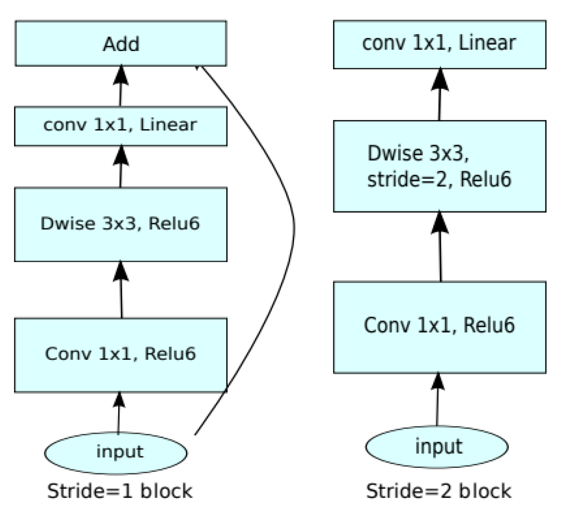
In the architecture of SSD MobileNetV2 FPN-Lite, MobileNetV2 is used as a base network, SSD as a detection network, and FPN-Lite as a feature extractor. Figure 1 shows that MobileNet V2 has three layers with two kinds of a block. The first block is a residue block with stride 1 while the second block is a stride 2 layer that is used to reduce the size. The first layer of MobileNet V2 is a 1 × 1 convolution layer with a Rectified Linear Unit with an upper cut-off at 6 or ReLU6, the second layer is a depth-wise convolution layer, and the third layer is a 1 × 1 convolution layer without non-linearity.

Many studies have already been conducted on object detection utilizing neural network hyperparameter tuning to increase model accuracy. Increasingly, SSD320 Mobilenet V2 FPNLite is being implemented in various applications such as road damage detection [8], traffic density [9], vulnerable road users [10], and real-time road-based object detection [11]. For robotic automation, SSD320 Mobilenet V2 FPNLite is used in various industries such as agriculture [12,13] and hospitality [14,15].

Many machine learning models previously developed had very large datasets that are not suitable for devices in the edge running real-time applications.

So far, not much research has been conducted on SSD MobileNet V2 FPN320-Lite on pick-and-place application in Raspberry Pi, especially on the hyperparameter and image enhancement optimisation, and thus our research aims to fill this gap. In addition, we investigate the effect of real-time inference of Raspberry Pi with an Edge Tensor Processing Unit (TPU) and validate with the other state-of-the-art lightweight models. Similar to Chen et al. [16], we adopt MS COCO 2017 as the primary benchmark for all experiments since it is more challenging and widely used. For SSD320 Mobilenet V2 FPNLite, the object detection’s mAP is 22.2%, according to TensorHub [17].

In this paper, we propose a new technique for object detection on an embedded system using SSD Mobilenet V2 FPN Lite with hyperparameter tuning and enhancing image properties to improve the mAP and detection scores of the deep learning models. The main contributions of the paper lie in the following:

• In comparison with the control group, we increase the mean Average Precision by 7% with an RGB saturation level of 3.5.
• We improve mean Average Precision to 46.63% and detection scores to 97% using a 416 × 416 aspect ratio, Learning Rate of 0.08, and quantized model for Edge TPU Standard.
• We achieve a detection rate of nearly 91% using RGB saturation and a robot approach distance of 45 cm.

2. Materials and Methods

This study is a continuation of our published works [18,19]. Figure 2 depicts the project setup for a smart and lean pick-and-place operation. Universal Robot 3 (UR3) is chosen to carry out the pick-and-place application as it has a payload of 3 kg, which is adequate for our small objects of cubes and cylinders. Raspberry Pi version 4B is tasked to run the lightweight deep learning model SSD MobileNet V2 FPN320-Lite to recognize objects in real-time. Using a webcam mounted on the robotic arm, a python program uses OpenCV to capture real-time video frames. When an object is detected by the “object detector” in the program, a bounding box with a detection score is drawn. Based on the predetermined threshold value of the object detection, the Raspberry Pi’s General Purpose Input Output (GPIO) pins are activated to control the robot arm to perform a specific pick-and-place operation. In order to increase the inference speed, we use a hardware USB accelerator Coral Edge Tensor Processing Unit (TPU).

The deep learning process flowchart is depicted in Figure 3, with a focus on hyperparameter optimisation for model training. The dataset is annotated using online tool Roboflow [20] and then trained in the cloud using the Google Colab platform [21]. A converter is then used to change the intermediate SavedModel into “.tflite” format for use with other models. The FlatBuffer format in which this model was saved allows for cross-platform serialization without the need for additional software. The Tflite model is then deployed to Raspberry Pi for robot arm control and inference. For our training process, we use Google Colab Professional with Tesla T4 GPU, which is based on Turing architecture. It is a GPU card based on the Turing architecture and targeted at deep learning model inference acceleration.

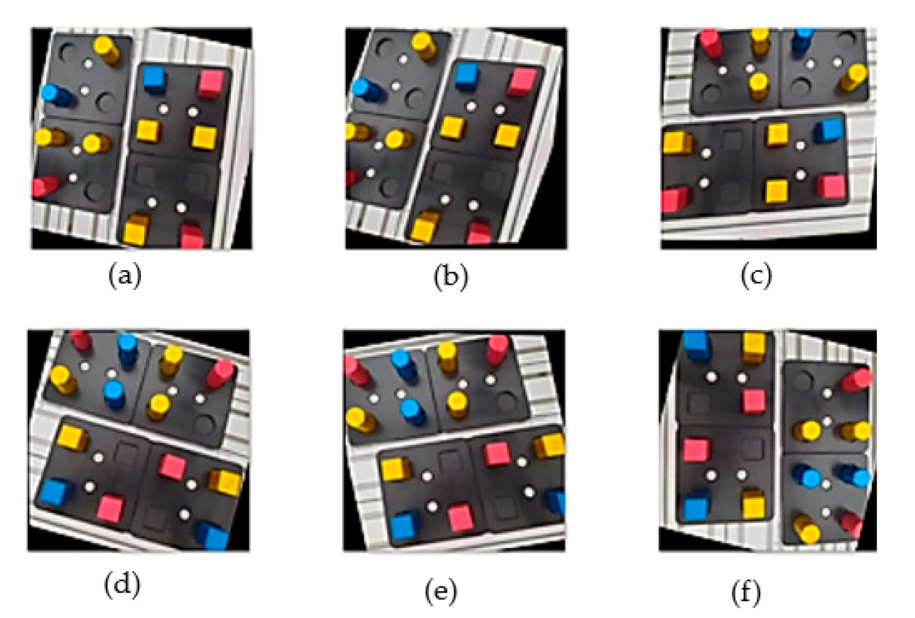
The project uses a custom dataset for the pick-and-place process, as shown in Figure 4. The dataset contains two types of workpieces: the cube and cylinder. The colours of the cube and cylinder are either red, blue, or yellow. To increase the number of images, 2 augmentation processes are executed, which are flip horizontal and vertical, as well as a rotation of ±15 degrees.

In

Table 1. Distribution of classes.

Classes	Number of Annotations	Distribution (%)
Blue cube	2079	14.10
Blue cylinder	2236	15.16
Red cube	2571	17.44
Red cylinder	2294	15.56
Yellow cube	2701	18.32
Yellow cylinder	2864	19.42

, we present the total distribution of the classes for the 6 classes. We observe that the overall distribution is even, as no single class is dominating the dataset. The overall distribution of all classes is 14 to 19%.

According to Google Developer [22], we have a moderate imbalance dataset if the minority class is 1 to 20% of the entire dataset. Since all the classes are within the band of 14% to 19% and there is no minority class, our dataset is considered as balanced.

We adopt the hyperparameter settings as shown in

Table 2. Hyperparameter settings.

Parameter	Setting
Aspect Ratio	320 (default), 416, 512, 640
Learning Rate	0.08 (default), 0.16
Number of Steps	5000, 10,000
Warmup Learning Rate	0.02666
Momentum Optimiser	0.9
Activation Function	Rectified linear unit (ReLU)

. The aspect ratio can be any multiple of 32, with a 320 × 320 set as the default aspect ratio. The number of training steps are set as a multiple of 2500. The maximum number of steps is 10,000. There are 2 Learning Rates used in the training, with a Learning Rate of 0.08 (LR0.08) set as the default. For optimisation, we use a weight decay of 0.001 and momentum of 0.9, similar to [2]. The mean Average Precision (mAP) and detection scores are used as metrics to evaluate performance of this model.

For faster inference, we utilize post-training quantization in which the model converts its weights from 32-bit floating-point values to 8-bit integer values. This allows the quantized model to run faster and occupy less memory without too much reduction in accuracy [23].

For our object detection, the evaluation criteria are the mean Average Precision (mAP) and detection scores. According to the COCO 2017 validation dataset, its mAP is the same as Average Precision in Tensorflow’s object detection.

The mAP metric we are using in this study is mAP_0.5:0.95, which is widely used as a benchmark to gauge the detector’s effectiveness [24]. mAP_0.5 represents the mAP value when the intersection over union (IoU) is 0.5 and mAP_0.5:0.95 represents the average mAP at different IoU thresholds (from 0.5 to 0.95 in steps of 0.05).

For our pick-and-place application, ARmax10 is chosen as the Recall value as we expect to have a maximum of 10 detections per pick-and-place application.

The formula of the mean Average Precision is given below:

$$mAP=\frac{1}{n}{\sum }_{k=1}^{k=n}{AP}_k$$

(1)

where AP_k is the Average Precision of class k, and n is the number of classes.

The standard deviation of the AP is calculated as follows:

$$\sigma =\sqrt{\frac{\sum {\left(x_i-\mu \right)}^2}{N}}$$

(2)

where $\sigma$ is the population standard deviation, N is the size of the population, x_i is the value of an AP, and μ is the population mean of all APs.

2.1. Learning Rate

Many studies attempt to use the largest Learning Rate that still allows for convergence, in order to improve training speed. However, a Learning Rate that is too large can be as slow as a Learning Rate that is too small, and a Learning Rate that is too large or too small can require more training time than one that is in an appropriate range [25].

For this reason, we train for just 2500 steps on the image of 640 × 640 pixels in order to speed up the training and be able to analyse the Learning Rate more quickly. We set the default Learning Rate as 0.08 (LR0.08) and double that to Learning Rate 0.16 (LR0.16) for both the non-quantized and quantized models. The overall Average Precision is calculated by averaging all of the APs from the six classes.

2.2. Aspect Ratio

Table 3. Datasets with different aspect ratios.

Dataset	Aspect Ratio	Training Images	Validation Images	Testing Images	Total Images
1	320 × 320	868	147	74	1089
2	416 × 416	868	147	74	1089
3	512 × 512	868	147	74	1089
4	640 × 640	868	147	74	1089

shows the configuration of 4 datasets with different aspect ratios. These datasets are identical, except for the aspect ratio. They have the same distribution of classes as listed in Table 1.

We use these datasets in order to evaluate which dataset produces the highest mean Average Precision. The default aspect ratio of 320 × 320 pixels is changed to 416 × 416, 512 × 520, and 640 × 640 by modifying the parameter Fixed Shape Resizer in the training configuration file.

We do not include the aspect ratio 640 × 640 as the image size is larger and the processing of large images presents significant computational challenges due to memory usage and computation requirements [26]. We use a commonly used data split ratio of 80:20 [27] where 868 images or 80% of the data are for training. The remaining 13% of images are for validation (147 images) and 7% are for testing (74 images).

2.3. Quantization and Edge TPU

Similar to Hsu et al. [28], we use the Edge Tensor Processing Unit (TPU) [29] to improve the inference speed. Edge TPU is a small Application-Specific Integrated Circuit (ASIC), designed for low-power devices. There are 2 versions of Edge TPU, namely Edge TPU Max and Edge TPU Standard. Both Edge versions are designed to enhance the performance of machine learning at the edge such as Raspberry Pi. It is important to note that both versions require the model to be quantized and the input must be an 8-bit quantized input tensor.

Edge TPU Max is able to accomplish more complicated and computationally demanding AI tasks than Edge TPU Standard with the overclocking of the processor. This increases the inferencing speed but also increases power consumption and causes the USB accelerator to become very hot, as the processor is overclocked.

Table 4. Edge TPU versions.

Edge Versions	Frequency	Power
Edge TPU Standard	4 trillion operations per second	500 mA at 5 V
Edge TPU Max	8 trillion operations per second	900 mA at 5 V

displays the Edge TPU specifications that are taken from the datasheet.

2.4. Image Enhancement

According to Shubham et al. [30], colour spaces such as the RGB model can be used to demarcate the objects against the background before incorporating them into the CNN model, thereby improving detection accuracy.

To study the effect of image enhancement using RGB saturation, we use Python Imaging Library (PIL) to modify the RGB saturation level of the dataset from 5 to 9. As shown in

Table 5. Training, Validation, and Test split.

Dataset Numbering	RGB Saturation	Enhanced Images with RGB Level	Non-Enhanced Images with RGB Level	Test Images	Total Images
5	1 (control)	39	290	74	560
6	1.5	39	290	74	560
7	2.5	39	290	74	560
8	3.5	39	290	74	560

, we add 39 enhancement images (less than 5% of total images) of level 1.5, 2.5, and 3.5 to the small dataset of 560 images.

The 560 images are extracted from Dataset 2, which is listed in Table 3. Dataset 2 is selected because, in comparison to the other datasets in Table 3, it has a higher mAP value. Datasets 5 to 8 are identical except for the different RGB saturation levels.

Our objective is to determine whether there is a visible increase in mAP due to RGB saturation despite the small size of the dataset. This is similar to Charloke [31], who used CNN on Raspberry Pi to monitor a codling moth population and achieve a high accuracy of 99% with a small dataset of 430 images. In addition, a small dataset allows for fast training time and practical data preparation [18].

Figure 5 illustrates the effect of the RGB saturation level on the images. The control group (Enhance 1) is the original image with no saturation added.

2.5. Approach Distance

In this study, we evaluate the effectiveness of RGB saturation with the variation of approach distance on the detection scores. As shown in Figure 6, the approach distance is calculated from the table base to the camera position. Altogether, there are 4 distance variations of 10 cm, from 35 cm to 65 cm. We use images of an aspect ratio of 416 × 416, as we have determined that it provides a higher mAP compared to other aspect ratios.

3. Results

3.1. The Effect of Learning Rate on Mean Average Precision

Table 6. Mean Average Precision with Learning Rate of 0.08.

Classes	Non-Quantized Model (%)	Quantized Model (%)
Blue cube	54.17	54.82
Blue cylinder	62.62	62.44
Red cube	28.13	28.69
Red cylinder	51.19	48.17
Yellow cube	36.33	37.80
Yellow cylinder	54.95	47.67
Overall	47.90	46.63
Standard deviation	11.84	10.96

shows the mAP for the model trained with LR0.08 while

Table 7. Mean Average Precision with Learning Rate of 0.16.

Classes	Non-Quantized Model (%)	Quantized Model (%)
Blue cube	44.65	34.16
Blue cylinder	73.39	74.98
Red cube	27.44	33.11
Red cylinder	34.30	45.30
Yellow cube	36.30	32.94
Yellow cylinder	63.71	61.72
Overall	46.63	47.00
Standard deviation	16.52	16.11

presents the mAP of the model trained with LR0.16. We observe that the mAP of the model trained with LR0.08 has a slight drop due to quantization but with a lower standard deviation. On the other hand, the mAP for LR0.16 has a slight increase due to quantization but with a higher standard deviation. Therefore, considering both mAP and standard deviation, we choose LR0.08 for our smart and lean pick-and-place system for better consistent model performance.

Figure 7 shows that the blue cylinder and yellow cylinder have higher mAP. This is expected for the yellow cylinder as it has more instances than the other classes. On the other hand, the blue cylinder has the highest mAP despite possessing one of the lowest number of instances. Strong-coloured objects, such as blue cylinders, have higher mAP due to their greater contrast to the background, providing more features for machine learning. This is consistent with our previous study [19].

3.2. The Effect of Aspect Ratio on Mean Average Precision

The default aspect ratio of 320 × 320 is set as the control dataset while 416 × 416 and 512 × 512 are set as test groups.

Table 8. Mean Average Precision with different aspect ratios (5000 training steps).

Classes	320 × 320	416 × 416	512 × 512
Blue cube	24.32	25.63	23.36
Blue cylinder	26.21	29.61	26.86
Red cube	46.36	53.62	38.22
Red cylinder	39.42	48.30	39.77
Yellow cube	44.30	54.81	38.93
Yellow cylinder	44.30	34.07	36.62
Overall	37.48	41.01	33.96
Comparison with default	-	+3.53	−3.52

shows the mean Average Precision of the respective aspect ratio with 5000 steps and

Table 9. Mean Average Precision with different aspect ratios (10000 training steps).

Classes	320 × 320	416 × 416	512 × 512
Blue cube	29.98	36.91	31.61
Blue cylinder	37.80	30.76	31.00
Red cube	27.90	47.36	47.19
Red cylinder	29.06	31.35	37.95
Yellow cube	44.16	45.57	41.05
Yellow cylinder	40.94	48.73	32.05
Overall	34.97	40.11	36.81
Comparison with default	-	+5.14	+1.84

is with 10,000 steps. The aspect ratio of 416 × 416 is used for the subsequent detection scores test as it has the highest overall mAP for both 5000 steps and 10,000 steps.

As mentioned in [17], the mAP on the COCO 2017 validation set is 22.2%. Because our overall mAP is higher than 22.2%, we can conclude that our detector has achieved good performance. In comparison with other works using SSD Mobilenet V2 such as Narkhede et al. 10 on Nvidia Jetson (another low-powered embedded device), our mAP for a quantized model with a Learning Rate of 0.08 is 46.63%, whereas theirs is 45%. Islam et al. [32] conducted a study on Raspberry Pi and their mAP was only 23.4%. Based on this, our results are better than those of the other two works.

3.3. The Effect of Quantization and Edge TPU on Detection Scores

The detection scores are obtained and presented in

Table 10. Detection scores with Learning Rate 0.08.

Classes	Non-Quantized (%)	Quantized (%)	Edge TPU Standard (%)	Edge TPU Max (%)
Blue cube	98	94	97	97
Blue cylinder	88	88	91	91
Red cube	93	94	94	93
Red cylinder	93	89	88	88
Yellow cube	93	94	92	94
Yellow cylinder	91	89	91	89
Overall	92.67	94	97	97

for Learning Rate 0.08 (LR0.08) and

Table 11. Detection scores with Learning Rate 0.16.

Classes	Non-Quantized (%)	Quantized (%)	Edge TPU Standard (%)	Edge TPU Max (%)
Blue cube	96	94	94	94
Blue cylinder	96	95	96	96
Red cube	97	96	96	97
Red cylinder	95	95	95	94
Yellow cube	97	97	91	97
Yellow cylinder	91	93	91	94
Overall	95.33	95.00	93.83	95.33

for Learning Rate 0.16 (LR0.16). We observe that the model trained with LR0.08 has higher detection scores than LR0.16. As mentioned in Zhai et al. [33], when doubling the default Learning Rate, the training diverges. This leads to training instability and, consequently, a reduced level of detection. A further analysis is conducted on Edge TPU Standard and Edge TPU Max for LR0.08, which have similar detection scores. We chose Edge TPU Standard for our future works, as Edge TPU Max overheats the Raspberry Pi over time and may result in performance loss.

3.4. The Effect of RGB Saturation on Mean Average Precision

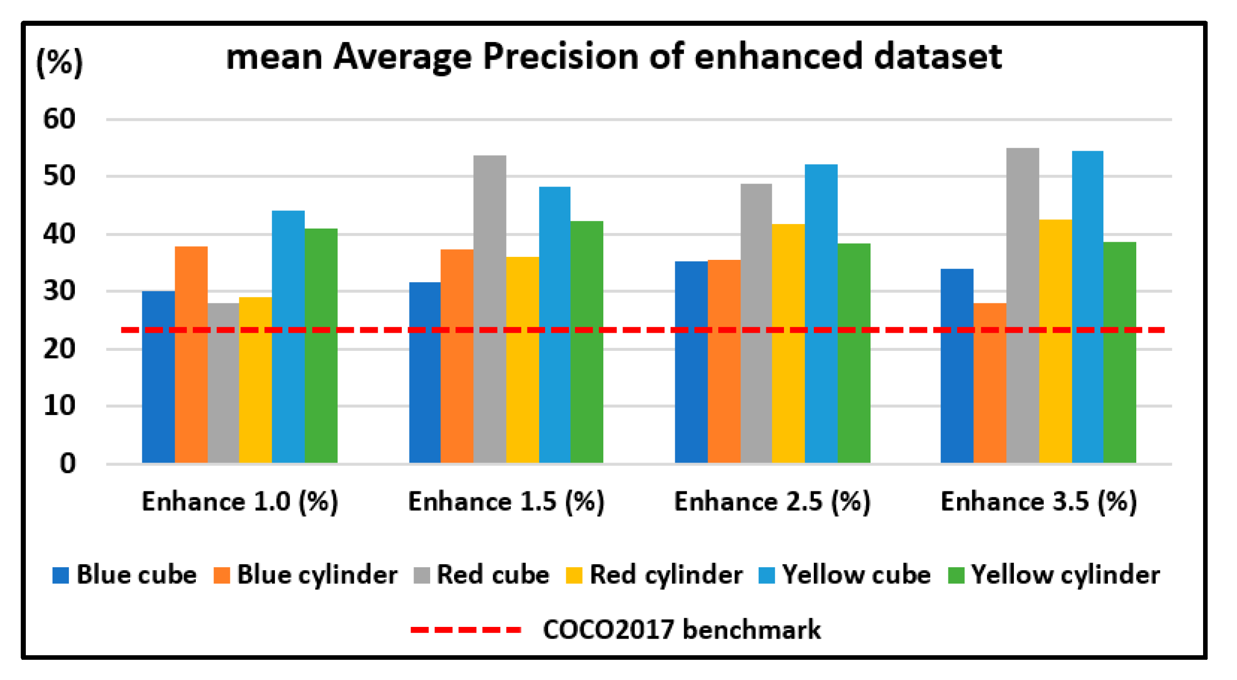
The results in

Table 12. Mean Average Precision with Enhanced Saturation Level.

Classes	Enhance 1.0 (%)	Enhance 1.5 (%)	Enhance 2.5 (%)	Enhance 3.5 (%)
Blue cube	29.98	31.71	35.1	34.02
Blue cylinder	37.8	37.33	35.36	27.9
Red cube	27.9	53.7	48.79	54.95
Red cylinder	29.06	36.07	41.79	42.4
Yellow cube	44.16	48.26	52.05	54.39
Yellow cylinder	40.94	42.28	38.27	38.54
Overall	34.97	41.56	41.89	42.03
Comparison over control group	-	+6.59	+6.92	+7.06
Comparison with COCO2017 validation dataset	+12.77	+19.36	+19.69	+19.83

showed that all the mAPs obtained are higher than the COCO 2017 validation dataset of 22.2% for SSD MobileNet V2. As expected, Enhance 3.5 has the biggest gain in mAP when compared to the control group of Enhance 1.0, as the features are more distinguishable. Enhance 3.5 has the highest increase with +7.06% over the control group and a nearly 20% increase over the COCO 2017 validation dataset.

As shown in Figure 8, all enhanced datasets including the control group have a higher mAP than the COCO 2017 validation dataset of 22.2% as a benchmark, which indicates improved object detection for our pick-and-place system.

3.5. The Effect of Quantization on Inference Speed

The inference speed of LR 0.08 and LR 0.16 is shown as Frame Per Seconds (FPS) in

Table 13. Inference speed of Non-Quantized vs. Quantized model.

Learning Rate	Non-Quantized (FPS)	Quantized (FPS)	Comparison of FPS
0.08	0.51	0.70	+0.19
0.16	0.48	0.58	+0.1

. We observe that the quantized model increases the FPS for both LR0.08 and LR0.16 by 0.1 to 0.19 FPS.

As depicted in

Table 14. Inference speed of Edge TPU Standard vs. Edge TPU Max.

Learning Rate	Edge TPU Standard (FPS)	Edge TPU Max (FPS)	Comparison of FPS
0.08	2.20	2.23	+0.03
0.16	2.16	2.26	+0.10

, compared to the non-quantized model, Edge TPU quadruples the FPS for both Learning Rates. In addition, the results show that Edge TPU Max outperforms Edge TPU Standard by 0.03 to 0.10 FPS. As Edge TPU Max consumes more power, we choose Edge TPU Standard of LR 0.08 for our future works.

To compare the FPS, we present inference speed in Figure 9, which shows that Edge TPU (Standard or Max) has higher inference speed than the normal quantized model.

3.6. The Effect of Approach Distance on Detection Scores

Table 15. Detection scores with variation of approach distance.

Enhancement Level	Classes	35 cm (%)	45 cm (%)	55 cm (%)	65 cm (%)
1.5	Blue-cube	94	98	96	81
	Blue-cyl	97	97	93	56
	Red-cube	95	96	78	-
	Red-cyl	93	97	93	90
	Yellow-cube	58	93	90	93
	Yellow-cyl	99	93	89	97
2.5	Blue-cube	98	97	95	80
	Blue-cyl	93	98	78	-
	Red-cube	95	91	86	-
	Red-cyl	85	92	75	51
	Yellow-cube	64	97	50	51
	Yellow-cyl	94	76	78	65
3.5	Blue-cube	96	96	88	70
	Blue-cyl	89	94	95	-
	Red-cube	96	89	88	-
	Red-cyl	94	96	93	71
	Yellow-cube	76	84	90	79
	Yellow-cyl	97	86	91	85
Average detection scores		89.61	92.78	85.89	74.54
Standard deviation		11.43	5.68	10.78	14.84

shows the result of real-time detection scores based on the distance variation of 10 cm from 35 cm to 65 cm for images with aspect ratio 416 × 416 with Enhance 3.5. The results showed that the system could still detect all the workpieces at a 45 cm approach distance. However, when the distance is at 65 cm, two thirds of the workpieces are undetected and unrecognized, marked as “-”.

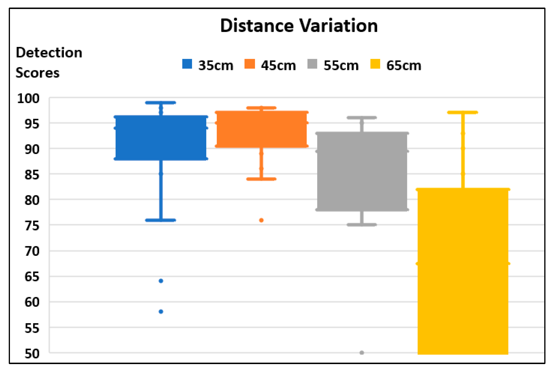
Figure 10 shows a boxplot summarizing the enhanced dataset. The detection scores for a distance of 45 cm have the smallest variation while those of a distance of 65 cm have the largest variation with the undetected workpiece. The figure also shows that distances of 35 cm and 55 cm have few outliers. Therefore, an approach distance of 45 cm is the most suitable approach distance for the robot to obtain the best detection scores.

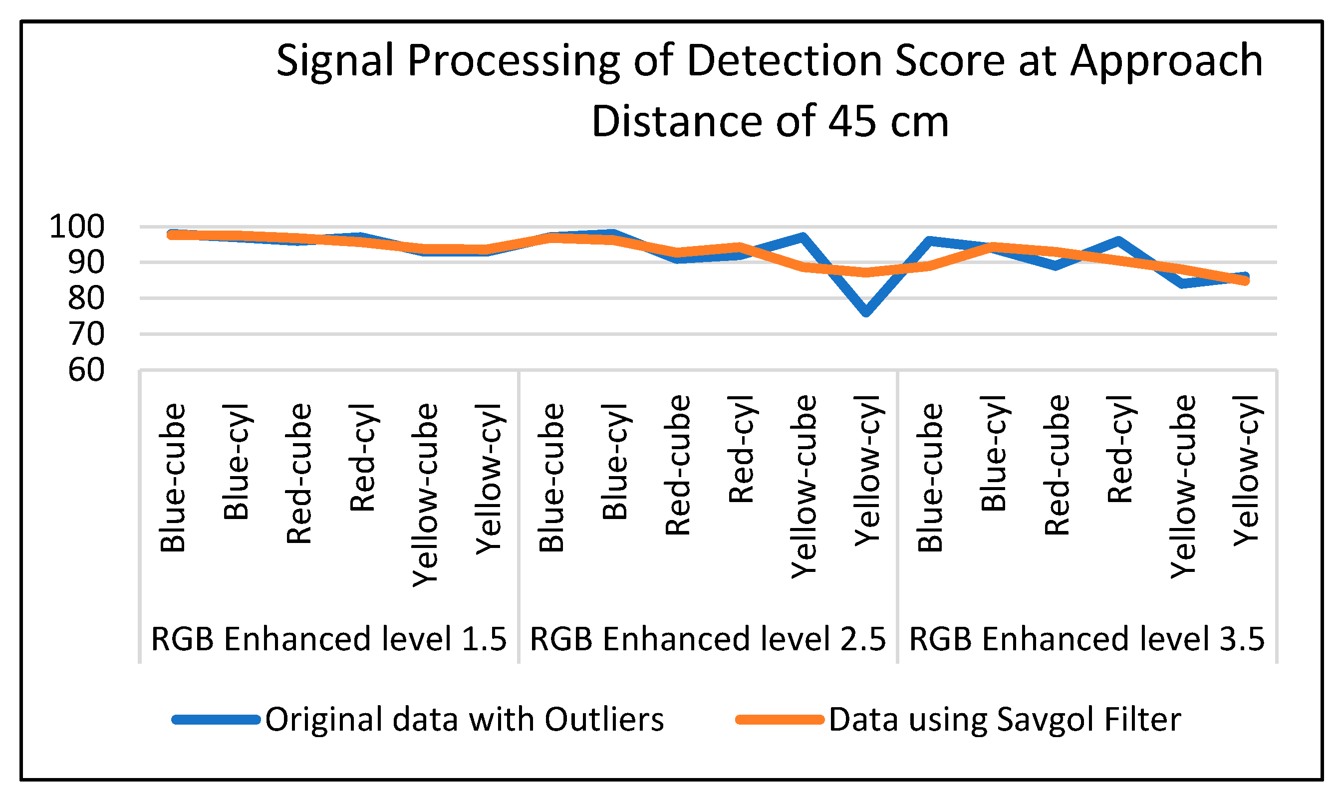
To enhance our results, we have added signal processing for the detection scores of an approach distance of 45 cm, as shown in

Table 16. Detection scores with optimum approach distance of 45 cm.

Enhancement Level	Classes	Original Data Scores with Outliers (%)	Processed Data Using Savgol Filter (%)
1.5	Blue-cube	98	97.63
	Blue-cyl	97	97.49
	Red-cube	96	96.77
	Red-cyl	97	95.63
	Yellow-cube	93	93.77
	Yellow-cyl	93	93.6
2.5	Blue-cube	97	96.83
	Blue-cyl	98	96.2
	Red-cube	91	92.71
	Red-cyl	92	94.23
	Yellow-cube	97	88.69
	Yellow-cyl	76	87.14
3.5	Blue-cube	96	88.97
	Blue-cyl	94	94.34
	Red-cube	89	92.94
	Red-cyl	96	90.51
	Yellow-cube	84	88.06
	Yellow-cyl	86	84.89

. We used the Savgol filter [34] to remove the outliers to the detection scores. According to F. Arzberger et. al. [35], the Savgol filter removes the effect of the outliers but preserves the signal tendency.

We use the basic Savgol filter with a window of 5 and a polynomial degree of 2 from the python SciPy library [36], which is a Python library used for scientific computing and technical computing. As shown in Figure 11, the graph has become smoother after we removed the outliers such as the low detection scores of RGB enhanced level 2.

4. Statistical Analysis

As we observed in Table 15 above, the detection scores of 45 cm and 55 cm are similar. Therefore, a statistical analysis is conducted to see whether there is a significant difference between the two groups of values. We utilize the Mann–Whitney U [37] method as it is one of the most commonly used non-parametric statistical tests. Developed by Mann and Whitney in 1947, this non-parametric test is frequently used for small samples of data that are not normally distributed.

In the Mann–Whitney U test, the null hypothesis states that the medians of the two respective groups are not different. An alternative hypothesis states that one median is larger than the other or that the two medians differ. If the null hypothesis is not rejected, it means that the median of each group of observations is similar. If the null hypothesis is rejected, it means the two medians differ.

We apply the Mann–Whitney U test to our 45 cm and 55 cm as the number of samples are small, less than 30, and the detection scores are not normally distributed. Our null hypothesis (H0) and alternative hypothesis (H1) are as follows:

H0 .

The median of APs is equal between 45 cm and 55 cm detection scores.

H1 .

The median of APs is not equal between 45 cm and 55 cm detection scores.

Using the SciPy function for the Mann–Whitney U test, we obtain a p-value of 0.787. Since the p-value (0.787) is above the 0.05 significance level, we fail to reject the null hypothesis.

We conclude that there is not enough evidence to suggest a significant difference in medians between the two datasets. As the standard deviation differs by 2.23, we recommend using 55 cm instead of 45 cm for more accurate inference.

5. Validation

For validation, we use dataset Enhance 3.5 and compare the mAP with two other state-of-the-art (SOTA) models. The SOTA models that used constrained object detection applications are EfficientDet-Lite0, which is the lightweight version of the EfficientDet family [38], and the Mobilenet Single Shot Multibox Detector or Mobilenet-SSD [39]. Mobilenet-SSD is the simpler version of SSD Mobilenet without the Feature Pyramid Network.

Table 17. Mean Average Precision of lightweight detectors.

Classes	SSD Mobilenet V2 FPNLite (%)	EfficientDet-Lite0 (%)	Mobilenet-SSD (%)
Blue cube	34.02	22.85	8.12
Blue cylinder	27.9	6.83	18.81
Red cube	54.95	13.27	28.52
Red cylinder	42.4	36.48	36.63
Yellow cube	54.39	4.70	22.64
Yellow cylinder	38.54	23.66	29.41
Overall mAP	42.03	17.96	24.02
Comparison	Nil	−24.07	−18.01

shows that the SSD Mobilenet V2 FPNLite model has much higher mAP compared to the other two detectors. This demonstrates that our detector is able to perform in accordance with the required specifications as well as meet the project objectives as a smart and lean pick-and-place system.

6. Discussion

Our project aims to develop a smart and lean pick-and-place system for a lightweight embedded microcontroller such as Raspberry Pi. The improvement in the Average Precision and detection scores depends on many factors and features; this study focused on the Learning Rate, model quantization, and use of a hardware accelerator to improve the mAP and inference speed. With the release of Raspberry Pi version 5 with faster inference speed, we should be able to use it to improve the inference speed. This is important for the pick-and-place operation in that the robot should react fast enough to pick up the objects.

Although our deep learning-based object detection model has demonstrated its ability to detect objects accurately, the computational requirements and real-time performance capabilities vary depending on the actual number of steps and other hyperparameter settings.

In addition, the results of the detection score are subject to ambient lighting and noise, which may vary significantly if the workplace is located in a poorly illuminated area or dusty area such as logistics and a warehouse. This is due to the fact that dust will obstruct the camera sensor, making it impossible for the model to accurately detect the features of the objects.

Our smart and lean pick-and-place robot can be deployed in agriculture and used to identify ripe fruit for harvesting. However, the colour characteristics of fruits change greatly under different lighting conditions and different growth stages. The shape characteristics are also impacted by different shooting angles of the camera. Therefore, the method of detecting fruits based on colour and shape features has certain limitations.

Furthermore, we should take note of the robot approach distance depending on the type of robot. For example, Universal Robot 3 has the arm reach of 50 cm and if the approach distance from the arm to the table base is bigger than 50 cm, the robot arm is not long enough to reach the objects. This would also affect the detection scores as our control algorithm utilizes high and consistent detection scores to establish the location of the workpiece and control the arm movement.

Our application can be extended to an edge computing environment as the Raspberry Pi is a low-power and low-computation computer that is close to a sensor. The smart-and-lean robot solution can be used for multi-object tracking for city surveillance in an edge computing environment with a flying robot or drone. In addition, our application can be used by a domestic autonomous robot as an IoT edge signal processing sensor, monitoring the condition of patients in a healthcare facility.

7. Conclusions

We presented a systematic method to determine the optimum aspect ratio and showed that an aspect ratio of 416 × 416 has higher mAP for both 5000 and 10,000 steps. By increasing the RGB saturation level of the images, we gain a 7% increase in mean Average Precision (mAP) when compared to the control group and a 20% increase in mAP when compared to the COCO2017 validation dataset of 22.2%. We showed that Learning Rate 0.08 with Edge TPU Standard provided a high detection score of 97%, as compared to Learning Rate 0.16 with Edge TPU Max. By combining the enhancement level and variation of distance, we proved that the optimum approach distance of 45 cm was able to obtain the maximum detection scores. The results are validated by comparing the performance with other SOTA embedded controllers—EfficientDet-Lite0 and Mobilenet-SSD.

Furthermore, our mAP for SSD Mobilenet V2 is 46.63%, whereas the mAPs of previous studies such as Narkhede et al. [10] and Islam et al. [32] are 45% and 23.4%, respectively. This demonstrates how our research has led to improved object detectors.

In the future, we plan to continue to develop a machine learning model with practical data preparation for embedded devices. Our goal is to further improve the inference time and Average Precision so that it can be used in applications such as the tightening of bolts and holes and the alignment of shipping containers. The use of machine learning models for pick-and-place applications on Raspberry Pi using SSD MobileNet V2 FPN320-Lite is relatively new and will provide useful insights toward developing vision systems that can perform reliably on real-world images.

References

- Singapore Busineess Review. Available online: https://sbr.com.sg/information-technology/news/time-saving-top-benefit-ai-singaporean-businesses-zoom (accessed on 3 January 2024).
- Lin, T.Y.; Goyal, P.; Girshick, R.; He, K.; Dollár, P. Focal loss for dense object detection. In Proceedings of the IEEE International Conference on Computer Vision, Venice, Italy, 22–29 October 2017. [Google Scholar]
- Aamir, S.M.; Ma, H.; Khan MA, A.; Aaqib, M. Real-Time Object Detection in Occluded Environment with Background Cluttering Effects Using Deep Learning. arXiv 2024, arXiv:2401.00986. [Google Scholar]
- Nurfirdausi, A.F.; Soekirno, S.; Aminah, S. Implementation of Single Shot Detector (SSD) MobileNet V2 on Disabled Patient’s Hand Gesture Recognition as a Notification System. In Proceedings of the 2021 International Conference on Advanced Computer Science and Information Systems (ICACSIS), Depok, Indonesia, 23–25 October 2021; pp. 1–6. [Google Scholar] [CrossRef]
- Ren, S.; He, K.; Girshick, R.; Sun, J. Faster r-cnn: Towards real-time object detection with region proposal networks. Adv. Neural Inf. Process. Syst. 2015, 28, 91–99. [Google Scholar] [CrossRef] [PubMed]
- Redmon, J.; Divvala, S.; Girshick, R.; Farhadi, A. You Only Look Once: Unified, Real-Time Object Detection. Available online: http://pjreddie.com/yolo/ (accessed on 20 January 2023).
- Sandler, M.; Howard, A.; Zhu, M.; Zhmoginov, A.; Chen, L.C. Mobilenetv2: Inverted residuals and linear bottlenecks. In Proceedings of the IEEE Conference on Computer Vision and Pattern Recognition, Salt Lake City, UT, USA, 18–22 June 2018. [Google Scholar]
- Aqsa, A.C.; Mahmudah, H.; Sudibyo, R.W. Detection and Classification of Road Damage Using CNN with Hyperparameter Optimization. In Proceedings of the 2022 6th International Conference on Informatics and Computational Sciences (ICICoS), Semarang, Indonesia, 28–29 September 2022. [Google Scholar]
- Biswas, D.; Su, H.; Wang, C.; Stevanovic, A.; Wang, W. An automatic traffic density estimation using Single Shot Detection (SSD) and MobileNet-SSD. Phys. Chem. Earth Parts A/B/C 2019, 110, 176–184. [Google Scholar] [CrossRef]
- Narkhede, M.; Chopade, N. Real-Time Detection of Vulnerable Road Users Using a Lightweight Object Detection Model. Int. J. Intell. Syst. Appl. Eng. 2024, 12, 129–135. [Google Scholar]
- Kumar, S.; Kumar, R. Real-Time Detection of Road-Based Objects using SSD MobileNet-v2 FPNlite with a new Benchmark Dataset. In Proceedings of the 2023 4th International Conference on Computing, Mathematics and Engineering Technologies (iCoMET), Sukkur, Pakistan, 17–18 March 2023; pp. 1–5. [Google Scholar]
- Yuan, T.; Lv, L.; Zhang, F.; Fu, J.; Gao, J.; Zhang, J.; Li, W.; Zhang, C.; Zhang, W. Robust Cherry Tomatoes Detection Algorithm in Greenhouse Scene Based on SSD. Agriculture 2020, 10, 160. [Google Scholar] [CrossRef]
- Magalhães, S.A.; Castro, L.; Moreira, G.; dos Santos, F.N.; Cunha, M.; Dias, J.; Moreira, A.P. Evaluating the Single-Shot MultiBox Detector and YOLO Deep Learning Models for the Detection of Tomatoes in a Greenhouse. Sensors 2021, 21, 3569. [Google Scholar] [CrossRef] [PubMed]
- Ramalingam, B.; Elara Mohan, R.; Balakrishnan, S.; Elangovan, K.; Félix Gómez, B.; Pathmakumar, T.; Devarassu, M.; Mohan Rayaguru, M.; Baskar, C. sTetro-Deep Learning Powered Staircase Cleaning and Maintenance Reconfigurable Robot. Sensors 2021, 21, 6279. [Google Scholar] [CrossRef] [PubMed]
- Teng, T.W.; Veerajagadheswar, P.; Ramalingam, B.; Yin, J.; Elara Mohan, R.; Gómez, B.F. Vision Based Wall Following Framework: A Case Study With HSR Robot for Cleaning Application. Sensors 2020, 20, 3298. [Google Scholar] [CrossRef] [PubMed]
- Chen, K.; Wang, J.; Pang, J.; Cao, Y.; Xiong, Y.; Li, X.; Sun, S.; Feng, W.; Liu, Z.; Xu, J.; et al. MMDetection: Open mmlab detection toolbox and benchmark. arXiv 2019, arXiv:1906.07155. [Google Scholar]
- Tensorflow Hub. Available online: https://tfhub.dev/tensorflow/ssd_mobilenet_v2/fpnlite_320x320/1 (accessed on 6 January 2024).
- Kee, E.; Chong, J.J.; Choong, Z.J.; Lau, M. A Comparative Analysis of Cross-Validation Techniques for a Smart and Lean Pick-and-Place Solution with Deep Learning. Electronics 2023, 12, 2371. [Google Scholar] [CrossRef]
- Kee, E.; Chong, J.J.; Choong, Z.J.; Lau, M. Development of Smart and Lean Pick-and-Place System Using EfficientDet-Lite for Custom Dataset. Appl. Sci. 2023, 13, 11131. [Google Scholar] [CrossRef]
- Roboflow. Available online: https://roboflow.com/ (accessed on 2 January 2024).
- Google Colab. Available online: https://colab.research.google.com/ (accessed on 2 January 2024).
- Google Developer. Available online: https://developers.google.com/machine-learning/data-prep/construct/sampling-splitting/imbalanced-data (accessed on 27 January 2024).
- Quantization. Available online: https://www.tensorflow.org/lite/performance/post_training_quantization (accessed on 26 December 2023).
- Padilla, R.; Passos, W.L.; Dias, T.L.B.; Netto, S.L.; da Silva, E.A.B. A Comparative Analysis of Object Detection Metrics with a Companion Open-Source Toolkit. Electronics 2021, 10, 279. [Google Scholar] [CrossRef]
- Wilson, D.; Martinez, T. The need for small learning rates on large problems. In Proceedings of the IJCNN’01. International Joint Conference on Neural Networks. Proceedings (Cat. No.01CH37222), Washington, DC, USA, 15–19 July 2001; Volume 1, pp. 115–119. [Google Scholar]
- Toma, A.C.; Panica, S.; Zaharie, D.; Petcu, D. Computational challenges in processing large hyperspectral images. In Proceedings of the 2012 5th Romania Tier 2 Federation Grid, Cloud & High Performance Computing Science (RQLCG), Cluj-Napoca, Romania, 25–27 October 2012. [Google Scholar]
- Joseph, V.R. Optimal ratio for data splitting. Stat. Anal. Data Min. ASA Data Sci. J. 2022, 15, 531–538. [Google Scholar] [CrossRef]
- Hsu, K.C.; Tseng, H.W. Accelerating applications using edge tensor processing units. In Proceedings of the International Conference for High Performance Computing, Networking, Storage and Analysis, St. Louis, MO, USA, 14–19 November 2021. [Google Scholar]
- Edge TPU. Available online: https://coral.ai/docs/ (accessed on 2 January 2024).
- Nain, S.; Mittal, N.; Hanmandlu, M. CNN-based plant disease recognition using colour space models. Int. J. Image Data Fusion 2024, 1–14. [Google Scholar] [CrossRef]
- Chakole, S.; Ukani, N. Low-Cost Vision System for Pick and Place application using camera and ABB Industrial Robot. In Proceedings of the 2020 11th International Conference on Computing, Communication and Networking Technologies (ICCCNT), Kharagpur, India, 1–3 July 2020. [Google Scholar]
- Bin Islam, R.; Akhter, S.; Iqbal, F.; Rahman, S.U.; Khan, R. Deep learning based object detection and surrounding environment description for visually impaired people. Heliyon 2023, 9, e16924. [Google Scholar] [CrossRef] [PubMed]
- Zhai, S.; Likhomanenko, T.; Littwin, E.; Busbridge, D.; Ramapuram, J.; Zhang, Y.; Gu, J.; Susskind, J.M. Stabilizing transformer training by preventing attention entropy collapse. In Proceedings of the International Conference on Machine Learning, PMLR, Honolulu, HI, USA, 23–29 July 2023. [Google Scholar]
- Savitzky, A.; Golay, M.J.E. Smoothing and differentiation of data by simplified least squares procedures. Anal. Chem. 1964, 36, 1627–1639. [Google Scholar] [CrossRef]
- Arzberger, F.; Wiecha, F.; Zevering, J.; Rothe, J.; Borrmann, D.; Montenegro, S.; Nüchter, A. Delta Filter-Robust Visual-Inertial Pose Estimation in Real-Time: A Multi-Trajectory Filter on a Spherical Mobile Mapping System. In Proceedings of the 2023 European Conference on Mobile Robots (ECMR), Coimbra, Portugal, 4–7 September 2023. [Google Scholar]
- Scipy Library. Available online: https://docs.scipy.org/doc/scipy/reference/generated/scipy.signal.savgol_filter.html (accessed on 6 February 2024).
- Mann, H.B.; Whitney, D.R. On a test of whether one of two random variables is stochastically larger than the other. Ann. Math. Stat. 1947, 18, 50–60. [Google Scholar] [CrossRef]
- Kamath, V.; Renuka, A. Performance Analysis of the Pretrained EfficientDet for Real-time Object Detection on Raspberry Pi. In Proceedings of the 2021 International Conference on Circuits, Controls and Communications (CCUBE), Bangalore, India, 23–24 December 2021; pp. 1–6. [Google Scholar] [CrossRef]
- Li, Y.; Huang, H.; Xie, Q.; Yao, L.; Chen, Q. Research on a Surface Defect Detection Algorithm Based on MobileNet-SSD. Appl. Sci. 2018, 8, 1678. [Google Scholar] [CrossRef]
Figure 1.
MobileNetV2 convolution blocks.
Figure 2.
Project setup of machine-vision-assisted pick-and-place solution: (a) webcam; (b) laptop running Colab; (c) Raspberry Pi; (d) collaborative robot; (e) Coral Edge TPU.
Figure 3.
CNN model building and training workflow.
Figure 4.
Augmentation of dataset with 2 to 16 instances: (a) flip vertical; (b) rotate clockwise +15 degrees; (c) flip horizontal; (d) rotate −15 degrees; (e) flip horizontal and rotate −15 degrees; (f) flip vertical and rotate +15 degrees.
Figure 5.
Variation of RGB saturation: (a) Level 1 (control group); (b) Level 1.5; (c) Level 2.5; (d) Level 3.5.
Figure 6.
Variation of approach distance.
Figure 7.
Comparison of Learning Rate and quantization.
Figure 8.
Mean Average Precision of enhanced dataset.
Figure 9.
Comparison of inference with quantization.
Figure 10.
Boxplot of detection scores.
Figure 11.
Signal processing of detection scores at approach distance of 45cm.