Digital Signal Processing (DSP)-Oriented Reduced-Complexity Algorithms for Calculating Matrix–Vector Products with Small-Order Toeplitz Matrices

Abstract

Toeplitz matrix–vector products are used in many digital signal processing applications. Direct methods for calculating such products require $N^2$ multiplications and $N(N-1)$ additions, where N denotes the order of the Toeplitz matrix. In the case of large matrices, this operation becomes especially time intensive. However, matrix–vector products with small-order Toeplitz matrices are of particular interest because small matrices often serve as kernels in modern digital signal processing algorithms. Perhaps reducing the number of arithmetic operations when calculating matrix–vector products in the case of small Toeplitz matrices gives less effect than of large ones, but this problem exists, and it needs to be solved. The traditional way to calculate such products is to use the fast Fourier transform algorithm. However, in the case of small-order matrices, it is advisable to use direct factorization of Toeplitz matrices, which leads to a reduction in arithmetic complexity. In this paper, we propose a set of reduced-complexity algorithms for calculating matrix–vector products with Toeplitz matrices of order $N=3,4,5,6,7,8,9$. The main emphasis will be on reducing multiplicative complexity since multiplication in most cases is more time-consuming than addition. This paper also provides assessments of the implementation of the developed algorithms on FPGAs.

1. Introduction

Structured matrices possess some inherent structure or pattern, which can be exploited to develop faster and more efficient algorithms for computing with them. Computing with structured matrices typically involves developing specialized algorithms that take advantage of the underlying structure of the matrix to reduce the computational complexity of matrix operations. Many fast algorithms have been developed for computing with structured matrices [1,2,3,4,5]. These algorithms can significantly reduce the computation complexity when implementing operations with such matrices. The Toeplitz matrix occupies a special place among structured matrices. This is due to the widespread use of matrix–vector transforms associated with these matrices when solving various applied problems. They appear in many areas, like in approximation theory [6], compressive sensing [7], image processing [8,9,10], filtering and estimating [11,12], signal processing [7,13,14,15], statistics [16,17], time series analysis [18], acoustic echo cancellation and active noise control [19,20,21], cryptography [22,23,24], deep neural networks [25,26,27,28,29,30,31], and many other areas [32,33,34,35,36,37,38]. As for the operations of matrix–vector multiplication with small-order Toeplitz matrices, they are, among other things, used in organizing the structures and computational processes of high-performance binary multipliers [22,39].

At present, a sufficient number of publications describe efficient methods for fast calculation of Toeplitz matrix–vector products [40,41,42]. Known fast algorithms are based on embedding such a matrix in a $2N\times 2N$ circulant matrix and calculating the matrix–vector product with the resulting matrix. Therefore, Toeplitz matrix–vector multiplication can be calculated as the product of a circulant matrix by a vector. This product can be computed using fast Fourier transform (FFT) algorithms [43]. These algorithms lead to data redundancy and require $O\left(NlogN\right)$ operations [44]. However, this approach involves rather complicated housekeeping and a relatively large number of multiplications and additions. What is more, these operations are performed on complex numbers.

Alternative efficient algorithms for multiplying a Toeplitz/Hankel matrix by a vector not based on FFT were discussed in [45,46]. Both of these methods, based on the Karatsuba multiplication method [47], have a computational complexity of $O\left(N^{lo{g}_{2}3}\right)$ multiplications and use only real arithmetic. One way or another, well-known publications mainly describe general approaches to rationalizing the computations of Toeplitz matrix–vector products and practically do not consider examples of constructing such algorithms for specific N. At the same time, developing such algorithms for specific N is of independent interest since such algorithms can be used as building blocks, contributing to unification in designing more complex algorithms.

In this article, we propose and describe in detail new rationalized algorithms for matrix–vector multiplication for Toeplitz matrices of orders $N=3,4,5,6,7,8,9$, which minimize the multiplication complexity compared to the conventional direct method, at the cost of some increase in additions. We emphasize that the reduced-complexity algorithm for the product of a matrix and a vector with a Toeplitz matrix for $N=2$ is well-known in the literature and therefore is not considered here.

The remainder of this paper is organized as follows. Section 2 explains the preliminary information about Toeplitz matrices. Section 3 describes the proposed algorithms for orders from $N=3$ to $N=9$. Section 4 evaluates our algorithms in terms of computational cost. Section 5 concludes this paper.

2. Preliminary Remarks

The Toeplitz matrix is a structural one and has the same values on each diagonal:

$${\mathbf{T}}_N=\left[\begin{array}{cccc}{t}_{N-1}& \dots & t_1& t_0\\ t_N& \cdots & t_2& t_1\\ ⋮& \ddots & \ddots & ⋮\\ t_{2N-2}& \cdots & t_N& t_{N-1}\end{array}\right].$$

(1)

The Toeplitz matrix–vector product can be represented as follows:

$${\mathbf{Y}}_{N\times 1}={\mathbf{T}}_N{\mathbf{X}}_{N\times 1},$$

(2)

where ${\mathbf{X}}_{N\times 1}={[x_0,x_1,\dots ,x_{N-1}]}^T$, ${\mathbf{Y}}_{N\times 1}={[y_0,y_1,\dots ,y_{N-1}]}^T$.

A direct application of the mathematical definition of matrix–vector multiplication (2), based on the multiplication of a dense matrix by a vector, yields an algorithm that, for real values, requires $N^2$ multiplications and $N(N-1)$ additions. In the remainder of this article, such an algorithm will be referred to as the direct method, and the designated number of arithmetic operations will refer to the case where real values are used. In the general case of complex value calculations, the corresponding quantities correspond to complex multiplications and additions. The problem is to find a way to factorize the matrix that will lead to a reduction in computation, which has been undertaken using the relationships presented in the paper ([48]).

3. Algorithms for Toeplitz Matrix–Vector Multiplication

3.1. Algorithm for $N=3$

Let it be necessary to calculate the matrix–vector product of the following form:

$$\left[\begin{array}{c}{y}_0\\ y_1\\ y_2\end{array}\right]=\left[\begin{array}{ccc}{t}_2& t_1& t_0\\ t_3& t_2& t_1\\ t_4& t_3& t_2\end{array}\right]\left[\begin{array}{c}{x}_0\\ x_1\\ x_2\end{array}\right].$$

(3)

The direct method of calculating the base matrix–vector product (3) requires 9 multiplications and 6 additions.

Proposition 1. 

To calculate the product (3), no more than 6 multiplications are required.

Proof. 

Let us introduce auxiliary matrices: the matrix ${\mathbf{P}}_{3\times 6}^{\left(3\right)}$ with the final summation operations performed to obtain the ${\mathbf{Y}}_{3\times 1}$ signals and the matrix ${\mathbf{T}}_{6\times 3}^{\left(3\right)}$ with the initial summation operations to prepare the corresponding signals to be multiplied by the diagonal matrix ${\mathbf{D}}_6^{\left(3\right)}$, in which the entries are the algebraic sums of entries of the Toeplitz matrix ${\mathbf{T}}_3$. In this paper, in matrices containing summation, such as ${\mathbf{P}}_{3\times 6}^{\left(3\right)}$ and ${\mathbf{T}}_{6\times 3}^{\left(3\right)}$, all zeros are omitted to improve readability.

$${\mathbf{P}}_{3\times 6}^{\left(3\right)}=\left[\begin{array}{cccccc}1& & & & 1& 1\\ & & 1& 1& 1& \\ 1& 1& 1& & & \end{array}\right],$$

$${\mathbf{T}}_{6\times 3}^{\left(3\right)}=\left[\begin{array}{ccc}1& & 1\\ 1& & \\ 1& 1& \\ & 1& \\ & 1& 1\\ & & 1\end{array}\right],$$

and

$${\mathbf{D}}_6^{\left(3\right)}=\mathrm{diag}\left(\begin{array}{cccc}{s}_0^{\left(3\right)},& s_1^{\left(3\right)},& \cdots ,& s_5^{\left(3\right)}\end{array}\right),$$

(4)

$$s_0^{\left(3\right)}=t_2,s_1^{\left(3\right)}=-t_2-t_3+t_4,$$

$$s_2^{\left(3\right)}=t_3,s_3^{\left(3\right)}=-t_1+t_2-t_3,$$

$$s_4^{\left(3\right)}=t_1,s_5^{\left(3\right)}=t_0-t_1-t_2.$$

Taking into account the introduced matrix constructions, expression (2) can be written in the following form:

$${\mathbf{Y}}_{3\times 1}={\mathbf{P}}_{3\times 6}^{\left(3\right)}{\mathbf{D}}_6^{\left(3\right)}{\mathbf{T}}_{6\times 3}^{\left(3\right)}{\mathbf{X}}_{3\times 1},$$

(5)

where

$$\begin{array}{cc}{\mathbf{X}}_{3\times 1}={[x_0,x_1,x_2]}^T,& {\mathbf{Y}}_{3\times 1}={[y_0,y_1,y_2]}^T.\end{array}$$

It is easy to see that the multiplicative complexity of calculating expression (5) is 6.

The correctness of expression (5) is confirmed by the truth of the expression

$${\mathbf{T}}_3={\mathbf{P}}_{3\times 6}^{\left(3\right)}{\mathbf{D}}_6^{\left(3\right)}{\mathbf{T}}_{6\times 3}^{\left(3\right)},$$

where ${\mathbf{T}}_3$ is a $3\times 3$ Toeplitz matrix (1). Expression (5) defines a reduced multiplicative complexity algorithm for calculating the matrix–vector product with a third-order Toeplitz matrix. □

Remark 1. 

The proposed algorithm (5) requires only 6 multiplications and 15 additions. In a number of practical applications, the entries of the Toeplitz matrix, i.e., $t_0,t_1,\dots ,t_4$, are constant numbers. Then, the entries of the matrix ${\mathbf{D}}_6^{\left(3\right)}$ (4) can be calculated in advance and stored in the calculator’s memory. For this case, the number of additions in the algorithm is reduced to 9. Thus, the proposed algorithm (5) applied to the calculation of the matrix–vector product (3) reduces 3 multiplication at the expense of 3 extra additions compared to the direct method.

Figure 1 shows the data flow diagram of the proposed algorithm (5). The initial and final additions follow from the matrices ${\mathbf{P}}_{3\times 6}^{\left(3\right)}$ and ${\mathbf{T}}_{3\times 6}^{\left(3\right)}$. The coefficients $s_i$ are derived from the entries $s_i^{\left(3\right)}$ of the matrix ${\mathbf{D}}_6^{\left(3\right)}$. For simplicity, superscripts on variables are omitted in all figures, as it is self-evident which variable is referenced in each case. This paper presents data flow diagrams in a left-to-right orientation, where straightforward lines within the illustrations represent data transfer operations. Circles in these diagrams represent multiplication operations, with the respective numerical factors inscribed inside. Points of convergence, marked with a bold dot, indicate summation. Additionally, dashed lines indicate data transfer operations with a simultaneous sign change. To maintain visual clarity, standard lines without arrows are employed.

3.2. Algorithm for $N=4$

Let it be necessary to calculate the matrix–vector product of the following form:

$$\left[\begin{array}{c}{y}_0\\ y_1\\ y_2\\ y_3\end{array}\right]=\left[\begin{array}{cccc}{t}_3& t_2& t_1& t_0\\ t_4& t_3& t_2& t_1\\ t_5& t_4& t_3& t_2\\ t_6& t_5& t_4& t_3\end{array}\right]\left[\begin{array}{c}{x}_0\\ x_1\\ x_2\\ x_3\end{array}\right].$$

(6)

The direct method of calculating this product requires 16 multiplications and 12 additions.

Proposition 2. 

To calculate the product (6), no more than 9 multiplications are required.

Proof. 

Let us introduce some auxiliary matrices, pre- and postaddition matrices:

$${\mathbf{P}}_{4\times 6}^{\left(4\right)}=\left[\begin{array}{cccccc}& 1& 1& & & \\ 1& & & 1& & \\ & & 1& & & 1\\ & & & 1& 1& \end{array}\right],$$

$$\begin{array}{cc}{\mathbf{P}}_{6\times 9}^{\left(4\right)}={\mathbf{I}}_3\otimes {\mathbf{P}}_{2\times 3}^{\left(4\right)},& {\mathbf{P}}_{2\times 3}^{\left(4\right)}=\left[\begin{array}{ccc}1& 1& \\ & 1& 1\end{array}\right],\end{array}$$

$$\begin{array}{cc}{\mathbf{T}}_{9\times 6}^{\left(4\right)}={\mathbf{I}}_3\otimes {\mathbf{T}}_{3\times 2}^{\left(4\right)},& {\mathbf{T}}_{3\times 2}^{\left(4\right)}=\left[\begin{array}{cc}1& \\ 1& 1\\ & 1\end{array}\right],\end{array}$$

$${\mathbf{T}}_{6\times 4}^{\left(4\right)}=\left[\begin{array}{cccc}& & 1& \\ & & & 1\\ & 1& & 1\\ 1& & 1& \\ 1& & & \\ & 1& & \end{array}\right],$$

and a diagonal matrix of multiplication factors ${\mathbf{D}}_9^{\left(4\right)}$, in which the entries are the algebraic sums of entries of the Toeplitz matrix ${\mathbf{T}}_4$:

$${\mathbf{D}}_9^{\left(4\right)}=\mathrm{diag}\left(\begin{array}{cccc}{s}_0^{\left(4\right)},& s_1^{\left(4\right)},& \cdots & s_8^{\left(4\right)}\end{array}\right),$$

(7)

$$s_0^{\left(4\right)}=w_0^{\left(4\right)}+w_1^{\left(4\right)},s_1^{\left(4\right)}=-w_0^{\left(4\right)},$$

$$s_2^{\left(4\right)}=t_0-t_2+w_0^{\left(4\right)},s_3^{\left(4\right)}=t_2-t_3,s_4^{\left(4\right)}=t_3,$$

$$s_5^{\left(4\right)}=t_4-t_3,s_6^{\left(4\right)}=-t_4+t_6+w_2^{\left(4\right)},s_7^{\left(4\right)}=-w_2^{\left(4\right)},$$

$$s_8^{\left(4\right)}=-w_1^{\left(4\right)}+w_2^{\left(4\right)},$$

where

$$w_0^{\left(4\right)}=-t_1+t_3,w_1^{\left(4\right)}=t_2-t_4,w_2^{\left(4\right)}=t_3-t_5,$$

and the sign ⊗″ denotes the Kronecker product [49].

Considering the matrices that have been introduced, expression (6) can be represented as follows:

$${\mathbf{Y}}_{4\times 1}={\mathbf{P}}_{4\times 6}^{\left(4\right)}{\mathbf{P}}_{6\times 9}^{\left(4\right)}{\mathbf{D}}_9^{\left(4\right)}{\mathbf{T}}_{9\times 6}^{\left(4\right)}{\mathbf{T}}_{6\times 4}^{\left(4\right)}{\mathbf{X}}_{4\times 1},$$

(8)

where

$$\begin{array}{c}{\mathbf{X}}_{4\times 1}={[x_0,x_1,x_2,x_3]}^T,\\ {\mathbf{Y}}_{4\times 1}={[y_0,y_1,y_2,y_3]}^T.\end{array}$$

It is easy to see that the multiplicative complexity of expression (8) is 9.

The correctness of expression (8) is confirmed by the truth of the following expression:

$${\mathbf{T}}_4={\mathbf{P}}_{4\times 6}^{\left(4\right)}{\mathbf{P}}_{6\times 9}^{\left(4\right)}{\mathbf{D}}_9^{\left(4\right)}{\mathbf{T}}_{9\times 6}^{\left(4\right)}{\mathbf{T}}_{6\times 4}^{\left(4\right)},$$

where ${\mathbf{T}}_4$ is a $4\times 4$ Toeplitz matrix (1). Expression (8) defines a reduced multiplicative complexity algorithm for calculating the matrix–vector product with a fourth-order Toeplitz matrix. □

Remark 2. 

The proposed algorithm requires only 9 multiplications and 26 additions. This gives, relative to the direct method, a reduction of 7 multiplications at the cost of an additional 14 additions. Suppose the entries of the matrix ${\mathbf{D}}_9^{\left(4\right)}$ (7) are constant values that can be precomputed and stored in the memory of a calculator. In that case, the implementation of the algorithm can be accomplished with only 15 additions, significantly reducing the computational requirements. Finally, we obtain a reduction in multiplications by 7 at the cost of 3 extra additions.

Figure 2 shows a data flow diagram of the proposed algorithm.

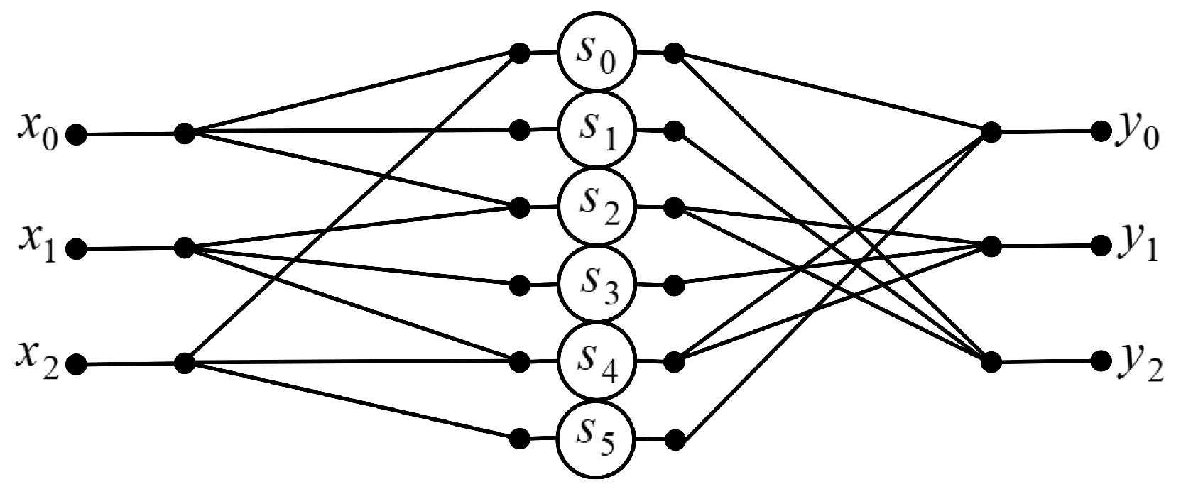
3.3. Algorithm for $N=5$

Let it be necessary to calculate the matrix–vector product of the following form:

$$\left[\begin{array}{c}{y}_0\\ y_1\\ y_2\\ y_3\\ y_4\end{array}\right]=\left[\begin{array}{ccccc}{t}_4& t_3& t_2& t_1& t_0\\ t_5& t_4& t_3& t_2& t_1\\ t_6& t_5& t_4& t_3& t_2\\ t_7& t_6& t_5& t_4& t_3\\ t_8& t_7& t_6& t_5& t_4\end{array}\right]\left[\begin{array}{c}{x}_0\\ x_1\\ x_2\\ x_3\\ x_4\end{array}\right].$$

(9)

The direct method of calculating this product requires 25 multiplications and 20 additions.

Proposition 3. 

To calculate the product (9), no more than 14 multiplications are required.

Proof. 

Let us introduce some auxiliary matrices, pre- and postaddition matrices:

$$\begin{array}{c}{\mathbf{P}}_{11\times 14}^{\left(5\right)}={\mathbf{I}}_4\oplus {\mathbf{I}}_3\otimes {\mathbf{P}}_{2\times 3}^{\left(4\right)}\oplus 1,\end{array}$$

$${\mathbf{T}}_{14\times 11}^{\left(5\right)}={\mathbf{I}}_4\oplus {\mathbf{I}}_3\otimes {\mathbf{T}}_{3\times 2}^{\left(4\right)}\oplus 1,$$

$$\begin{array}{c}{\mathbf{T}}_{11\times 5}^{\left(5\right)}=\left[\begin{array}{ccccc}1& & & & \\ 1& & & & 1\\ 1& & 1& & \\ 1& 1& & & \\ & 1& & 1& \\ & & 1& & 1\\ & 1& & & \\ & & 1& & \\ & & & 1& \\ & & & & 1\\ 1& & & 1& \end{array}\right],\end{array}$$

and a diagonal matrix of multiplication factors:

$${\mathbf{D}}_{14}^{\left(5\right)}=\mathrm{diag}\left(\begin{array}{cccc}{s}_0^{\left(5\right)},& s_1^{\left(5\right)},& \cdots ,& s_{13}^{\left(5\right)}\end{array}\right),$$

(10)

$$s_0^{\left(5\right)}=-t_4-t_7+t_8+w_3^{\left(5\right)},s_1^{\left(5\right)}=t_4,s_2^{\left(5\right)}=t_6,$$

$$s_3^{\left(5\right)}=t_7,s_4^{\left(5\right)}=w_0^{\left(5\right)},s_5^{\left(5\right)}=t_3,s_6^{\left(5\right)}=w_2^{\left(5\right)},$$

$$s_7^{\left(5\right)}=t_6-t_5-t_4+t_3-t_7,s_8^{\left(5\right)}=t_5-t_3,$$

$$s_9^{\left(5\right)}=t_4-w_2^{\left(5\right)}+w_3^{\left(5\right)},s_{10}^{\left(5\right)}=t_2-t_5+w_1^{\left(5\right)},$$

$$s_{11}^{\left(5\right)}=t_1-t_3,s_{12}^{\left(5\right)}=t_0-t_2+w_1^{\left(5\right)},s_{13}^{\left(5\right)}=t_5,$$

where

$$w_0^{\left(5\right)}=-t_3+t_4,w_1^{\left(5\right)}=-t_1-w_0^{\left(5\right)},w_2^{\left(5\right)}=t_2-t_3,$$

$$w_3^{\left(5\right)}=-t_5-t_6,$$

and the sign ⊕″ denotes the direct sum of matrices [50].

Considering the matrix constructions introduced earlier, expression (9) can be reformulated as follows:

$${\mathbf{Y}}_{5\times 1}={\mathbf{P}}_{5\times 11}^{\left(5\right)}{\mathbf{P}}_{11\times 14}^{\left(5\right)}{\mathbf{D}}_{14}^{\left(5\right)}{\mathbf{T}}_{14\times 11}^{\left(5\right)}{\mathbf{T}}_{11\times 5}^{\left(5\right)}{\mathbf{X}}_{5\times 1},$$

(11)

where

$$\begin{array}{c}{\mathbf{X}}_{5\times 1}={[x_0,x_1,x_2,x_3,x_4]}^T,\\ {\mathbf{Y}}_{5\times 1}={[y_0,y_2,y_3,y_3,y_4]}^T.\end{array}$$

It is easy to see that the multiplicative complexity of computing expression (11) is 14.

The correctness of expression (11) is confirmed by the truth of the following expression:

$${\mathbf{T}}_5={\mathbf{P}}_{5\times 11}^{\left(5\right)}{\mathbf{P}}_{11\times 14}^{\left(5\right)}{\mathbf{D}}_{14}^{\left(5\right)}{\mathbf{T}}_{14\times 11}^{\left(5\right)}{\mathbf{T}}_{11\times 5}^{\left(5\right)},$$

where ${\mathbf{T}}_5$ is a $5\times 5$ Toeplitz matrix. Expression (11) defines a reduced multiplicative complexity algorithm for calculating the matrix–vector product with a fifth-order Toeplitz matrix. □

Remark 3. 

The proposed algorithm requires only 14 multiplications and 45 additions. This gives, relative to the direct method, a reduction of 11 multiplications at the cost of an additional 25 additions. When the entries of the matrix ${\mathbf{D}}_{14}^{\left(5\right)}$ (10) are constant numbers that can be precalculated and stored in the calculator’s memory, the implementation of the algorithm (11) requires only 27 additions, effectively reducing the computational complexity. Finally, we obtain a reduction in multiplications by 11 at the cost of 7 extra additions.

Figure 3 shows a data flow diagram of the proposed algorithm.

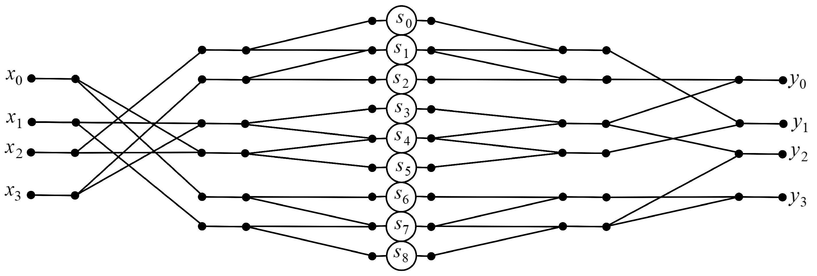
3.4. Algorithm for $N=6$

Let it be necessary to calculate the matrix–vector product of the following form:

$$\left[\begin{array}{c}{y}_0\\ y_1\\ y_2\\ y_3\\ y_4\\ y_5\end{array}\right]=\left[\begin{array}{cccccc}{t}_5& t_4& t_3& t_2& t_1& t_0\\ t_6& t_5& t_4& t_3& t_2& t_1\\ t_7& t_6& t_5& t_4& t_3& t_2\\ t_8& t_7& t_6& t_5& t_4& t_3\\ t_9& t_8& t_7& t_6& t_5& t_4\\ t_{10}& t_9& t_8& t_7& t_6& t_5\end{array}\right]\left[\begin{array}{c}{x}_0\\ x_1\\ x_2\\ x_3\\ x_4\\ x_5\end{array}\right].$$

(12)

The direct method of calculating this product requires 36 multiplications and 30 additions.

Proposition 4. 

To calculate the product (12), no more than 18 multiplications are required.

Proof. 

Let us introduce auxiliary matrices:

$$\begin{array}{cc}{\mathbf{P}}_{6\times 9}^{\left(6\right)}=\left[\begin{array}{ccc}{\mathbf{0}}_3& {\mathbf{I}}_3& {\mathbf{I}}_3\\ {\mathbf{I}}_3& {\mathbf{I}}_3& {\mathbf{0}}_3\end{array}\right],& {\mathbf{P}}_{9\times 18}^{\left(6\right)}={\mathbf{I}}_3\otimes {\mathbf{P}}_{3\times 6}^{\left(3\right)}\end{array},$$

and

$${\mathbf{T}}_{18\times 9}^{\left(6\right)}={\mathbf{I}}_3\otimes {\mathbf{T}}_{6\times 3}^{\left(3\right)},$$

$${\mathbf{T}}_{9\times 6}^{\left(6\right)}\left[\begin{array}{cccccc}1& & & & & \\ & 1& & & & \\ & & 1& & & \\ 1& & & 1& & \\ & 1& & & 1& \\ & & 1& & & 1\\ & & & 1& & \\ & & & & 1& \\ & & & & & 1\end{array}\right],$$

$${\mathbf{D}}_{18}^{\left(6\right)}=\mathrm{diag}\left(\begin{array}{cccc}{s}_0^{\left(6\right)},& s_1^{\left(6\right)},& \cdots ,& s_{17}^{\left(6\right)}\end{array}\right),$$

(13)

$$s_0^{\left(6\right)}=w_0^{\left(6\right)},s_1^{\left(6\right)}=t_{10}-w_0^{\left(6\right)}+w_2^{\left(6\right)},$$

$$s_2^{\left(6\right)}=-t_6+t_9,s_3^{\left(6\right)}=t_4+w_0^{\left(6\right)}+w_2^{\left(6\right)},$$

$$s_4^{\left(6\right)}=-t_4+t_7,s_5^{\left(6\right)}=-t_8+w_3^{\left(6\right)}-w_4^{\left(6\right)},s_6^{\left(6\right)}=t_5,$$

$$s_7^{\left(6\right)}=-w_3^{\left(6\right)},s_8^{\left(6\right)}=t_6,s_9^{\left(6\right)}=-t_4+t_5-t_6,$$

$$s_{10}^{\left(6\right)}=t_4,s_{11}^{\left(6\right)}=-w_5^{\left(6\right)},s_{12}^{\left(6\right)}=w_6^{\left(6\right)},$$

$$s_{13}^{\left(6\right)}=-t_2-w_4^{\left(6\right)}+w_3^{\left(6\right)},s_{14}^{\left(6\right)}=t_3-t_6,$$

$$s_{15}^{\left(6\right)}=-t_1+t_6-w_4^{\left(6\right)}+w_6^{\left(6\right)},s_{16}^{\left(6\right)}=t_1-t_4,$$

$$s_{17}^{\left(6\right)}=t_0-t_1-t_2+w_5^{\left(6\right)},$$

where

$$w_0^{\left(6\right)}=-t_5+t_8,w_1^{\left(6\right)}=t_6-t_7,$$

$$w_2^{\left(6\right)}=-t_9+w_1^{\left(6\right)},w_3^{\left(6\right)}=t_5+w_1^{\left(6\right)},w_4^{\left(6\right)}=t_3-t_4,$$

$$w_5^{\left(6\right)}=t_5+w_4^{\left(6\right)},w_6^{\left(6\right)}=t_2-t_5.$$

Taking into account the introduced matrix constructions, expression (12) can be written in the following form:

$${\mathbf{Y}}_{6\times 1}={\mathbf{P}}_{6\times 9}^{\left(6\right)}{\mathbf{P}}_{9\times 18}^{\left(6\right)}{\mathbf{D}}_{18}^{\left(6\right)}{\mathbf{T}}_{18\times 9}^{\left(6\right)}{\mathbf{T}}_{9\times 6}^{\left(6\right)}{\mathbf{X}}_{6\times 1},$$

(14)

where

$$\begin{array}{c}{\mathbf{X}}_{6\times 1}={[x_0,x_1,x_2,x_3,x_4,x_5]}^T,\\ {\mathbf{Y}}_{6\times 1}={[y_0,y_2,y_3,y_3,y_4,y_5]}^T.\end{array}$$

It is easy to see that the multiplicative complexity of calculating expression (14) is 18.

The correctness of expression (14) can be checked by a simple substitution:

$${\mathbf{T}}_6={\mathbf{P}}_{6\times 9}^{\left(6\right)}{\mathbf{P}}_{9\times 18}^{\left(6\right)}{\mathbf{D}}_{18}^{\left(6\right)}{\mathbf{T}}_{18\times 9}^{\left(6\right)}{\mathbf{T}}_{9\times 6}^{\left(6\right)},$$

where ${\mathbf{T}}_6$ is a $6\times 6$ Toeplitz matrix. Expression (14) defines a reduced multiplicative complexity algorithm for calculating the matrix–vector product with a sixth-order Toeplitz matrix. □

Remark 4. 

The proposed algorithm (14) requires only 18 multiplications and 75 additions. Suppose the entries of the matrix ${\mathbf{D}}_{18}^{\left(6\right)}$ (13) are constant values that can be precomputed and stored in the memory of a calculator. In that case, the implementation of the algorithm can be accomplished with only 33 additions, significantly reducing the computational requirements. Thus, the proposed algorithm (14) applied to the calculation of the matrix–vector product (12) reduces 18 multiplications at the expense of 3 extra additions compared to the direct method.

Figure 4 shows a data flow diagram of the proposed algorithm.

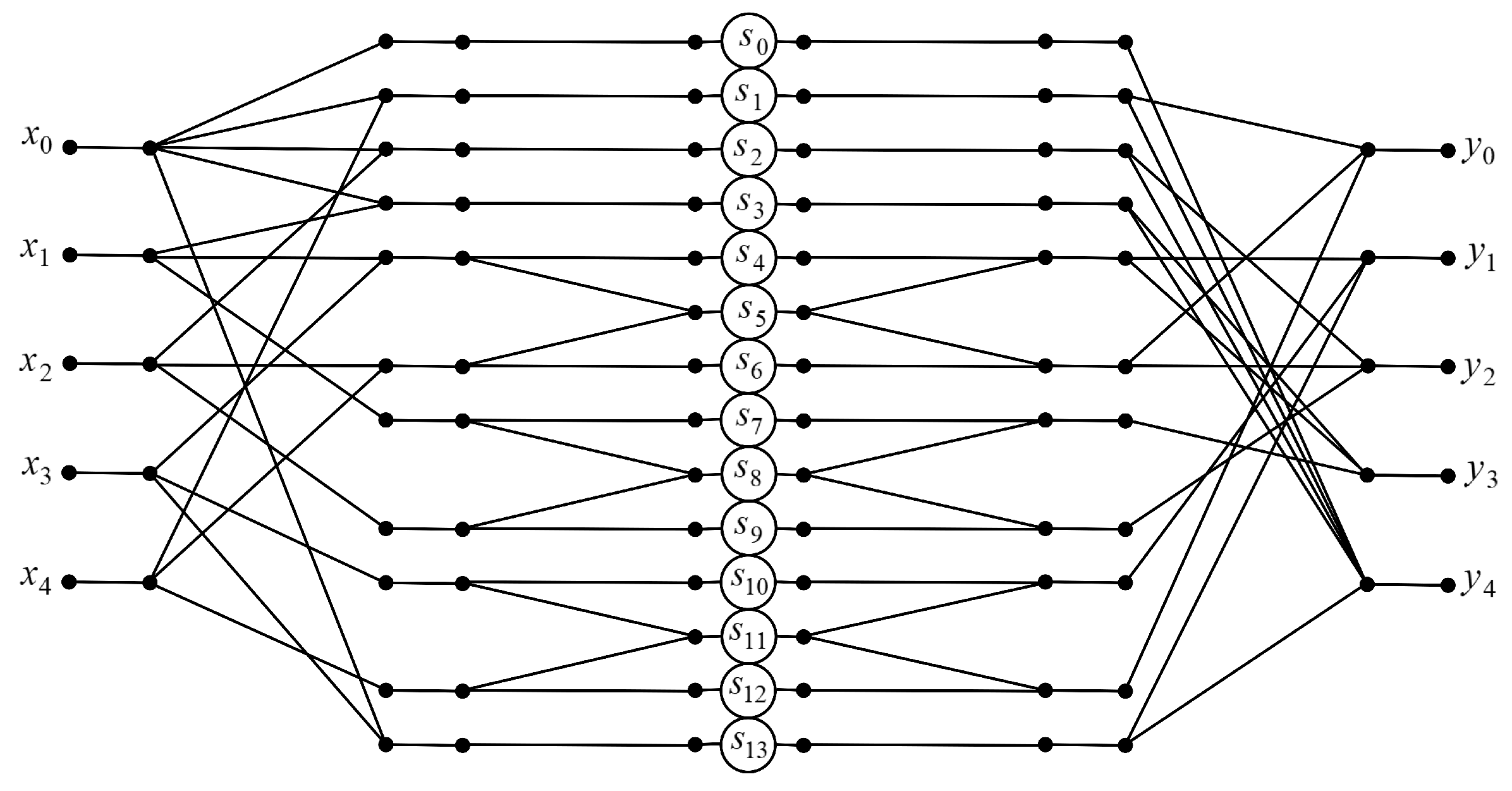
3.5. Algorithm for $N=7$

Let it be necessary to calculate the matrix–vector product of the following form:

$$\left[\begin{array}{c}{y}_0\\ y_1\\ y_2\\ y_3\\ y_4\\ y_5\\ y_6\end{array}\right]=\left[\begin{array}{ccccccc}{t}_6& t_5& t_4& t_3& t_2& t_1& t_0\\ t_7& t_6& t_5& t_4& t_3& t_2& t_1\\ t_8& t_7& t_6& t_5& t_4& t_3& t_2\\ t_9& t_8& t_7& t_6& t_5& t_4& t_3\\ t_{10}& t_9& t_8& t_7& t_6& t_5& t_4\\ t_{11}& t_{10}& t_9& t_8& t_7& t_6& t_5\\ t_{12}& t_{11}& t_{10}& t_9& t_8& t_7& t_6\end{array}\right]\left[\begin{array}{c}{x}_0\\ x_1\\ x_2\\ x_3\\ x_4\\ x_5\\ x_6\end{array}\right].$$

(15)

The direct method of calculating this product requires 49 multiplications and 42 additions.

Proposition 5. 

To calculate the product (15), no more than 25 multiplications are required.

Proof. 

Let us introduce auxiliary matrices:

$${\mathbf{P}}_{16\times 25}^{\left(7\right)}={\mathbf{I}}_4\oplus {\mathbf{P}}_{3\times 6}^{\left(3\right)}\oplus {\mathbf{I}}_2\oplus {\mathbf{P}}_{3\times 6}^{\left(3\right)}\oplus 1\oplus {\mathbf{P}}_{3\times 6}^{\left(3\right)},$$

$$\begin{array}{c}\hfill {\mathbf{P}}_{7\times 16}^{\left(7\right)}=\left[\begin{array}{cccccccccccccccc}& 1& & & 1& & & & & & & & & 1& & \\ & & 1& & & 1& & & & & & & & & 1& \\ & & & & & & 1& & & & & & 1& & & 1\\ & & & & 1& & & & 1& 1& & & & & & \\ & & & & & 1& & 1& & & 1& & & & & \\ & & & 1& & & 1& & & & & 1& & & & \\ 1& 1& 1& 1& & & & 1& 1& & & & 1& & \end{array}\right],\end{array}$$

$$\begin{array}{c}{\mathbf{T}}_{16\times 7}^{\left(7\right)}=\left[\begin{array}{ccccccc}1& & & & & & \\ 1& & & & & & 1\\ 1& & & & & 1& \\ 1& 1& & & & & \\ & 1& & & 1& & \\ & & 1& & & 1& \\ & & & 1& & & 1\\ 1& & 1& & & & \\ 1& & & 1& & & \\ & 1& & & & & \\ & & 1& & & & \\ & & & 1& & & \\ 1& & & & 1& & \\ & & & & 1& & \\ & & & & & 1& \\ & & & & & & 1\end{array}\right]\end{array},$$

$${\mathbf{T}}_{25\times 16}^{\left(7\right)}={\mathbf{I}}_4\oplus {\mathbf{T}}_{6\times 3}^{\left(3\right)}\oplus {\mathbf{I}}_2\oplus {\mathbf{T}}_{6\times 3}^{\left(3\right)}\oplus 1\oplus {\mathbf{T}}_{6\times 3}^{\left(3\right)},$$

and

$${\mathbf{D}}_{25}^{\left(7\right)}=\mathrm{diag}\left(\begin{array}{cccc}{s}_0^{\left(7\right)},& s_1^{\left(7\right)},& \cdots ,& s_{24}^{\left(7\right)}\end{array}\right),$$

(16)

$$s_0^{\left(7\right)}=-t_6-t_{10}+t_{12}+w_0^{\left(7\right)},s_1^{\left(7\right)}=t_6,s_2^{\left(7\right)}=t_7,$$

$$s_3^{\left(7\right)}=t_{11},s_4^{\left(7\right)}=t_5,s_5^{\left(7\right)}=-w_1^{\left(7\right)}+t_7,$$

$$s_6^{\left(7\right)}=t_6,s_7^{\left(7\right)}=-t_4+t_5-t_6,s_8^{\left(7\right)}=t_4,$$

$$s_9^{\left(7\right)}=-t_5-w_2^{\left(7\right)},s_{10}^{\left(7\right)}=t_{10},s_{11}^{\left(7\right)}=t_9,$$

$$s_{12}^{\left(7\right)}=-t_5+t_8,s_{13}^{\left(7\right)}=t_{10}+w_0^{\left(7\right)}+w_1^{\left(7\right)},$$

$$s_{14}^{\left(7\right)}=-t_6+t_9,s_{15}^{\left(7\right)}=-t_7+t_8-t_9-t_{10}-s_7^{\left(7\right)},$$

$$s_{16}^{\left(7\right)}=-t_4+t_7,s_{17}^{\left(7\right)}=-t_9+w_3^{\left(7\right)},s_{18}^{\left(7\right)}=t_8,$$

$$s_{19}^{\left(7\right)}=t_2-t_5,s_{20}^{\left(7\right)}=-t_2+w_3^{\left(7\right)},s_{21}^{\left(7\right)}=t_3-t_6,$$

$$s_{22}^{\left(7\right)}=-t_1+t_2-t_3-t_7-s_7^{\left(7\right)},s_{23}^{\left(7\right)}=t_1-t_4,$$

$$s_{24}^{\left(7\right)}=t_0-t_1-t_2-t_6-s_9^{\left(7\right)},$$

where

$$w_0^{\left(7\right)}=-t_7-t_8-t_9-t_{11},w_1^{\left(7\right)}=t_5+t_6,$$

$$w_2^{\left(7\right)}=-t_3+t_4,w_3^{\left(7\right)}=-t_8-s_5^{\left(7\right)}+w_2^{\left(7\right)}.$$

Taking into account the introduced matrix constructions, expression (3) can be written in the following form:

$${\mathbf{Y}}_{7\times 1}={\mathbf{P}}_{7\times 16}^{\left(7\right)}{\mathbf{P}}_{16\times 25}^{\left(7\right)}{\mathbf{D}}_{25}^{\left(7\right)}{\mathbf{T}}_{25\times 16}^{\left(7\right)}{\mathbf{T}}_{16\times 7}^{\left(7\right)}{\mathbf{X}}_{7\times 1}$$

(17)

where

$$\begin{array}{c}{\mathbf{X}}_{7\times 1}={[x_0,x_1,x_2,x_3,x_4,x_5,x_6]}^T,\\ {\mathbf{Y}}_{7\times 1}={[y_0,y_2,y_3,y_3,y_4,y_5,y_6]}^T.\end{array}$$

It is easy to see that the multiplicative complexity of calculating expression (17) is 25.

The correctness of expression (17) can be checked by a simple substitution:

$${\mathbf{T}}_7={\mathbf{P}}_{7\times 16}^{\left(7\right)}{\mathbf{P}}_{16\times 25}^{\left(7\right)}{\mathbf{D}}_{25}^{\left(7\right)}{\mathbf{T}}_{25\times 16}^{\left(7\right)}{\mathbf{T}}_{16\times 7}^{\left(7\right)},$$

where ${\mathbf{T}}_7$ is a $7\times 7$ Toeplitz matrix. Expression (17) defines a reduced multiplicative complexity algorithm for calculating the matrix–vector product with a seventh-order Toeplitz matrix. □

Remark 5. 

The proposed algorithm (17) requires only 25 multiplications and 87 additions. When the entries of the matrix ${\mathbf{D}}_{25}^{\left(7\right)}$ (16) are constant numbers that can be precalculated and stored in the calculator’s memory, the implementation of the algorithm (17) requires only 51 additions, effectively reducing the computational complexity. Finally, we obtain a reduction in multiplications by 24 at the cost of 9 extra additions.

Figure 5 shows a data flow diagram of the proposed algorithm.

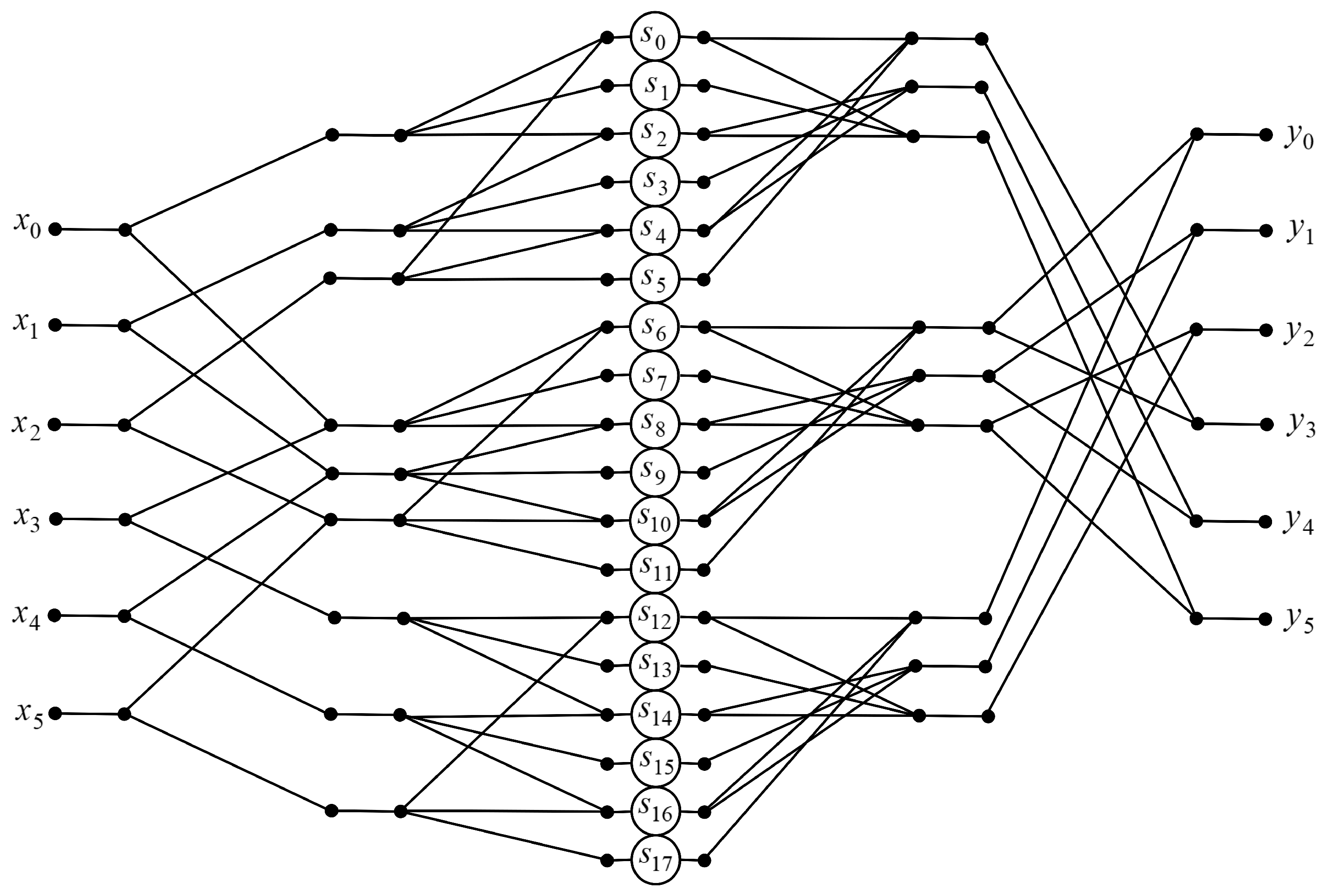
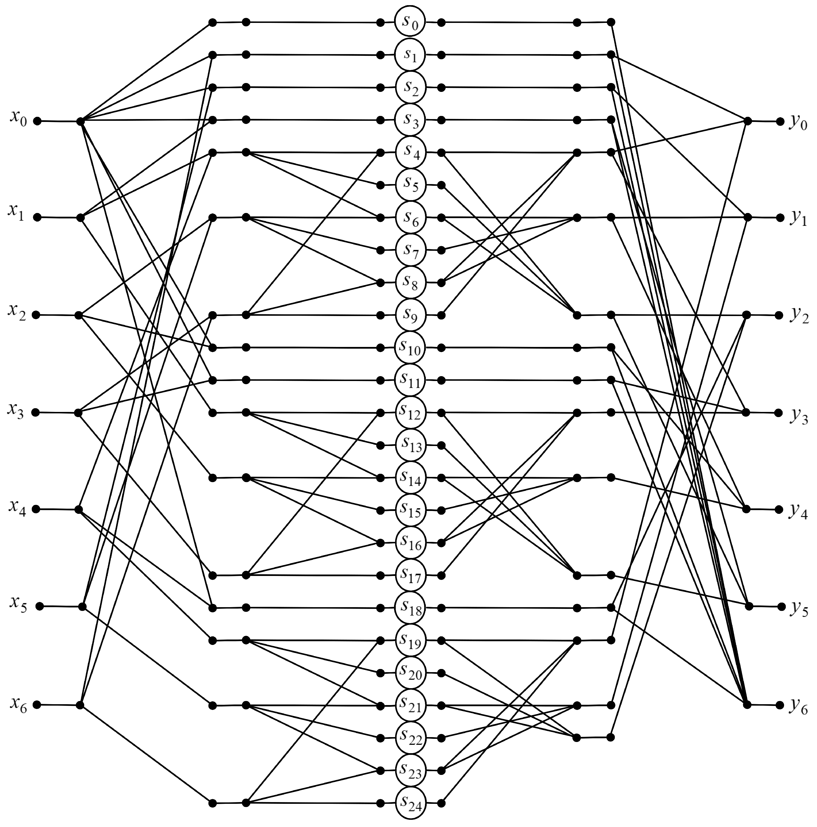
3.6. Algorithm for $N=8$

Let it be necessary to calculate the matrix–vector product of the following form:

$$\left[\begin{array}{c}{y}_0\\ y_1\\ y_2\\ y_3\\ y_4\\ y_5\\ y_6\\ y_7\end{array}\right]=\left[\begin{array}{cccccccc}{t}_7& t_6& t_5& t_4& t_3& t_2& t_1& t_0\\ t_8& t_7& t_6& t_5& t_4& t_3& t_2& t_1\\ t_9& t_8& t_7& t_6& t_5& t_4& t_3& t_2\\ t_{10}& t_9& t_8& t_7& t_6& t_5& t_4& t_3\\ t_{11}& t_{10}& t_9& t_8& t_7& t_6& t_5& t_4\\ t_{12}& t_{11}& t_{10}& t_9& t_8& t_7& t_6& t_5\\ t_{13}& t_{12}& t_{11}& t_{10}& t_9& t_8& t_7& t_6\\ t_{14}& t_{13}& t_{12}& t_{11}& t_{10}& t_9& t_8& t_7\end{array}\right]\left[\begin{array}{c}{x}_0\\ x_1\\ x_2\\ x_3\\ x_4\\ x_5\\ x_6\\ x_7\end{array}\right].$$

(18)

The direct method of calculating this product requires 64 multiplications and 56 additions.

Proposition 6. 

To calculate the product (18), no more than 27 multiplications are required.

Proof. 

Let us introduce auxiliary matrices:

$$\begin{array}{cc}{\mathbf{P}}_{8\times 12}^{\left(8\right)}={\mathbf{P}}_{2\times 3}^{\left(4\right)}\otimes {\mathbf{I}}_4,& {\mathbf{P}}_{12\times 18}^{\left(8\right)}={\mathbf{I}}_3\otimes {\mathbf{P}}_{4\times 6}^{\left(8\right)},\end{array}$$

$$\begin{array}{cc}{\mathbf{P}}_{4\times 6}^{\left(8\right)}={\mathbf{P}}_{2\times 3}^{\left(4\right)}\otimes {\mathbf{I}}_2,& {\mathbf{P}}_{18\times 27}^{\left(8\right)}={\mathbf{I}}_9\otimes {\mathbf{P}}_{2\times 3}^{\left(4\right)},\end{array}$$

and

$$\begin{array}{cc}{\mathbf{T}}_{27\times 18}^{\left(8\right)}={\mathbf{I}}_9\otimes {\mathbf{T}}_{3\times 2}^{\left(4\right)},& {\mathbf{T}}_{18\times 12}^{\left(8\right)}={\mathbf{I}}_3\otimes {\mathbf{T}}_{6\times 4}^{\left(8\right)},\end{array}$$

$${\mathbf{T}}_{6\times 4}^{\left(8\right)}={\mathbf{T}}_{3\times 2}^{\left(4\right)}\otimes {\mathbf{I}}_2,$$

$$\begin{array}{c}{\mathbf{T}}_{12\times 8}^{\left(8\right)}=\left[\begin{array}{cccccccc}& & & & & & & 1\\ & & & & & & 1& \\ & & & & & 1& & \\ & & & & 1& & & \\ & & & 1& & & & 1\\ & & 1& & & & 1& \\ & 1& & & & 1& & \\ 1& & & & 1& & & \\ & & & 1& & & & \\ & & 1& & & & & \\ & 1& & & & & & \\ 1& & & & & & & \end{array}\right],\end{array}$$

$${\mathbf{D}}_{27}^{\left(8\right)}=\mathrm{diag}\left(\begin{array}{cccc}{s}_0^{\left(8\right)},& s_1^{\left(8\right)},& \cdots ,& s_{26}^{\left(8\right)}\end{array}\right),$$

(19)

$$s_0^{\left(8\right)}=t_0+w_0^{\left(8\right)}-w_1^{\left(8\right)},s_1^{\left(8\right)}=t_1-t_3-s_{10}^{\left(8\right)},$$

$$s_2^{\left(8\right)}=t_8+w_0^{\left(8\right)}+w_1^{\left(8\right)},s_3^{\left(8\right)}=w_1^{\left(8\right)}-s_4^{\left(8\right)},$$

$$s_4^{\left(8\right)}=t_3-t_7,s_5^{\left(8\right)}=-s_4^{\left(8\right)}+w_2^{\left(8\right)},$$

$$s_6^{\left(8\right)}=-t_2+s_4^{\left(8\right)}+w_2^{\left(8\right)}+w_4^{\left(8\right)},s_7^{\left(8\right)}=-s_4^{\left(8\right)}-w_3^{\left(8\right)},$$

$$s_8^{\left(8\right)}=-t_{10}-s_5^{\left(8\right)}+w_4^{\left(8\right)},s_9^{\left(8\right)}=t_4-t_5-s_{12}^{\left(8\right)},$$

$$s_{10}^{\left(8\right)}=t_5-t_7,s_{11}^{\left(8\right)}=t_6-t_8-s_{10}^{\left(8\right)},$$

$$s_{12}^{\left(8\right)}=t_6-t_7,s_{13}^{\left(8\right)}=t_7,s_{14}^{\left(8\right)}=t_8-t_7,$$

$$s_{15}^{\left(8\right)}=-s_{12}^{\left(8\right)}+w_5^{\left(8\right)},s_{16}^{\left(8\right)}=t_9-t_7,$$

$$s_{17}^{\left(8\right)}=t_7-t_8+w_6^{\left(8\right)},s_{18}^{\left(8\right)}=-t_4+t_6-t_{10}+w_5^{\left(8\right)}+w_7^{\left(8\right)},$$

$$s_{19}^{\left(8\right)}=t_9-w_7^{\left(8\right)},s_{20}^{\left(8\right)}=-s_{11}^{\left(8\right)}+w_6^{\left(8\right)}+w_8^{\left(8\right)},$$

$$s_{21}^{\left(8\right)}=t_{10}-t_{11}-s_{12}^{\left(8\right)},s_{22}^{\left(8\right)}=t_{11}-t_7,$$

$$s_{23}^{\left(8\right)}=-s_{14}^{\left(8\right)}-w_8^{\left(8\right)},s_{24}^{\left(8\right)}=t_{12}-t_{13}-s_{21}^{\left(8\right)}-w_5^{\left(8\right)},$$

$$s_{25}^{\left(8\right)}=-t_{11}+t_{13}-s_{16}^{\left(8\right)},$$

$$s_{26}^{\left(8\right)}=-t_{13}+t_{14}+s_{14}^{\left(8\right)}-w_6^{\left(8\right)}+w_8^{\left(8\right)},$$

where

$$w_0^{\left(8\right)}=-t_1+t_3-t_4+s_{10}^{\left(8\right)},w_1^{\left(8\right)}=t_2-t_6,$$

$$w_2^{\left(8\right)}=t_4-t_8,w_3^{\left(8\right)}=-t_5+t_9,w_4^{\left(8\right)}=t_6+w_3^{\left(8\right)},$$

$$w_5^{\left(8\right)}=t_8-t_9,w_6^{\left(8\right)}=-t_9+t_{10},w_7^{\left(8\right)}=t_{11}+s_{10}^{\left(8\right)},$$

$$w_8^{\left(8\right)}=t_{11}-t_{12}.$$

Taking into account the introduced matrix constructions, expression (18) can be written in the following form:

$${\mathbf{Y}}_{8\times 1}={\mathbf{P}}_{8\times 12}^{\left(8\right)}{\mathbf{P}}_{12\times 18}^{\left(8\right)}{\mathbf{P}}_{18\times 27}^{\left(8\right)}{\mathbf{D}}_{27}^{\left(8\right)}{\mathbf{T}}_{27\times 18}^{\left(8\right)}{\mathbf{T}}_{18\times 12}^{\left(8\right)}{\mathbf{T}}_{12\times 8}^{\left(8\right)}{\mathbf{X}}_{8\times 1},$$

(20)

where

$$\begin{array}{c}{\mathbf{X}}_{8\times 1}={[x_0,x_1,x_2,x_3,x_4,x_5,x_6,x_7]}^T,\\ {\mathbf{Y}}_{8\times 1}={[y_0,y_2,y_3,y_3,y_4,y_5,y_6,y_7]}^T.\end{array}$$

It is easy to see that the multiplicative complexity of calculating expression (20) is 27.

The correctness of expression (20) can be checked by a simple substitution:

$${\mathbf{T}}_8={\mathbf{P}}_{8\times 12}^{\left(8\right)}{\mathbf{P}}_{12\times 18}^{\left(8\right)}{\mathbf{P}}_{18\times 27}^{\left(8\right)}{\mathbf{D}}_{27}^{\left(8\right)}{\mathbf{T}}_{27\times 18}^{\left(8\right)}{\mathbf{T}}_{18\times 12}^{\left(8\right)}{\mathbf{T}}_{12\times 8}^{\left(8\right)},$$

where ${\mathbf{T}}_8$ is an $8\times 8$ Toeplitz matrix. Expression (20) defines a reduced multiplicative complexity algorithm for calculating the matrix–vector product with an eighth-order Toeplitz matrix. □

Remark 6. 

The proposed algorithm (20) requires only 27 multiplications and 114 additions. Suppose the entries of the matrix ${\mathbf{D}}_{27}^{\left(8\right)}$ (19) are constant values that can be precomputed and stored in the memory of a calculator. In that case, the implementation of the algorithm can be accomplished with only 57 additions, significantly reducing the computational requirements. Finally, we obtain a reduction in multiplications by 37 at the cost of one extra addition compared to the direct method.

Figure 6 shows a data flow diagram of the proposed algorithm.

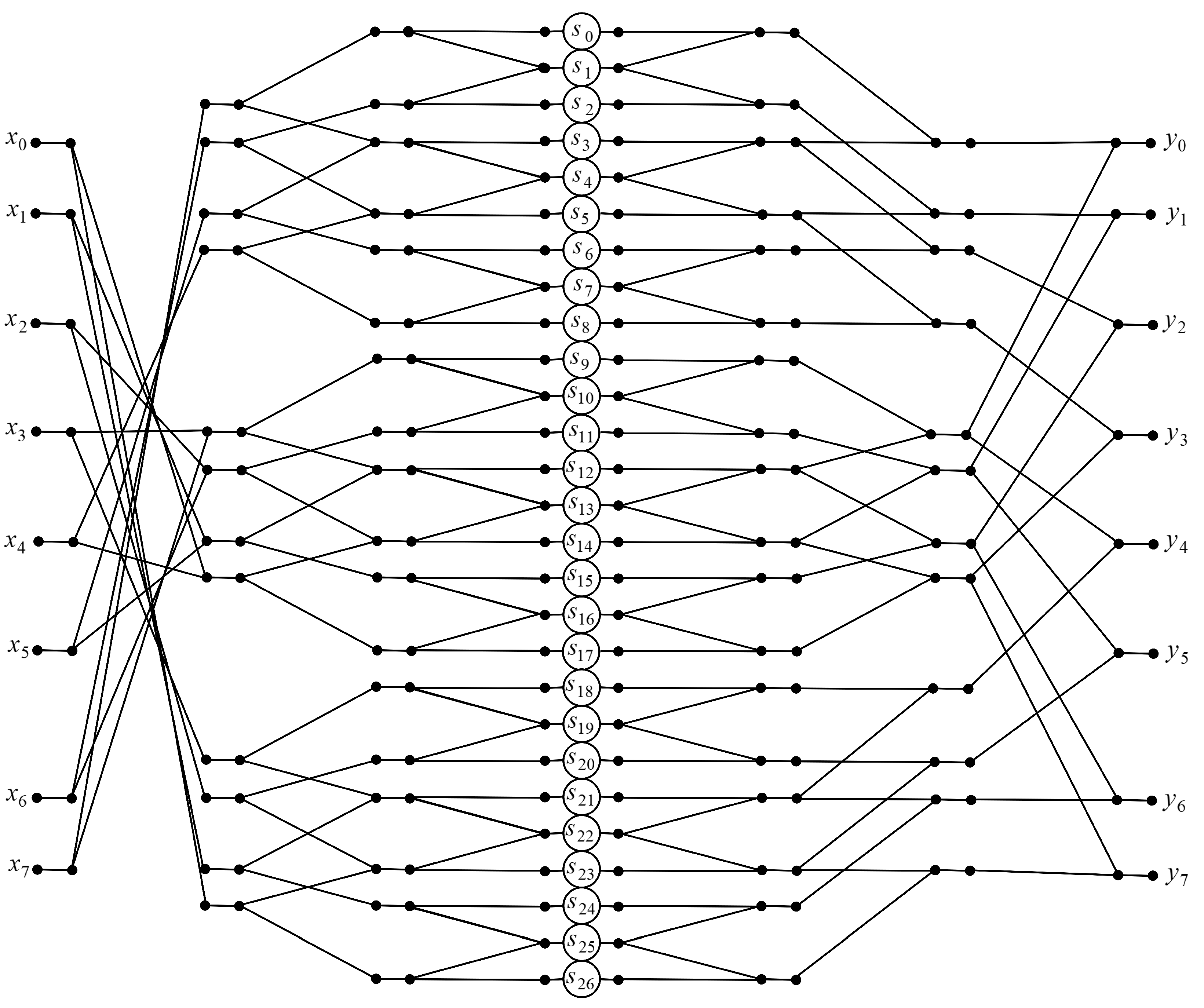
3.7. Algorithm for $N=9$

Let it be necessary to calculate the matrix–vector product of the following form:

$$\begin{array}{c}\hfill \left[\begin{array}{c}{y}_0\\ y_1\\ y_2\\ y_3\\ y_4\\ y_5\\ y_6\\ y_7\\ y_8\end{array}\right]=\left[\begin{array}{ccccccccc}{t}_8& t_7& t_6& t_5& t_4& t_3& t_2& t_1& t_0\\ t_9& t_8& t_7& t_6& t_5& t_4& t_3& t_2& t_1\\ t_{10}& t_9& t_8& t_7& t_6& t_5& t_4& t_3& t_2\\ t_{11}& t_{10}& t_9& t_8& t_7& t_6& t_5& t_4& t_3\\ t_{12}& t_{11}& t_{10}& t_9& t_8& t_7& t_6& t_5& t_4\\ t_{13}& t_{12}& t_{11}& t_{10}& t_9& t_8& t_7& t_6& t_5\\ t_{14}& t_{13}& t_{12}& t_{11}& t_{10}& t_9& t_8& t_7& t_6\\ t_{15}& t_{14}& t_{13}& t_{12}& t_{11}& t_{10}& t_9& t_8& t_7\\ t_{16}& t_{15}& t_{14}& t_{14}& t_{12}& t_{11}& t_{11}& t_9& t_8\end{array}\right]\left[\begin{array}{c}{x}_0\\ x_1\\ x_2\\ x_3\\ x_4\\ x_5\\ x_6\\ x_7\\ x_8\end{array}\right].\end{array}$$

(21)

The direct method of calculating this product requires 81 multiplications and 72 additions.

Proposition 7. 

To calculate the product (21), no more than 36 multiplications are required.

Proof. 

Let us introduce auxiliary matrices:

$${\mathbf{T}}_{18\times 9}^{\left(9\right)}=\left[\begin{array}{ccccccccc}1& & & & & & 1& & \\ & 1& & & & & & 1& \\ & & 1& & & & & & 1\\ 1& & & 1& & & & & \\ & 1& & & 1& & & & \\ & & 1& & & 1& & & \\ 1& & & & & & & & \\ & 1& & & & & & & \\ & & 1& & & & & & \\ & & & 1& & & & & \\ & & & & 1& & & & \\ & & & & & 1& & & \\ & & & 1& & & 1& & \\ & & & & 1& & & 1& \\ & & & & & 1& & & 1\\ & & & & & & 1& & \\ & & & & & & & 1& \\ & & & & & & & & 1\end{array}\right],$$

$$\begin{array}{cc}{\mathbf{T}}_{36\times 18}^{\left(9\right)}={\mathbf{I}}_6\otimes {\mathbf{T}}_{6\times 3}^{\left(3\right)},& {\mathbf{T}}_{6\times 3}^{\left(3\right)}=\left[\begin{array}{ccc}1& & 1\\ 1& & \\ 1& 1& \\ & 1& \\ & 1& 1\\ & & 1\end{array}\right]\end{array},$$

$${\mathbf{P}}_{18\times 36}^{\left(9\right)}={\mathbf{I}}_6\otimes {\mathbf{P}}_{3\times 6}^{\left(9\right)},$$

$${\mathbf{P}}_{3\times 6}^{\left(9\right)}=\left[\begin{array}{cccccc}1& & & & 1& 1\\ & & 1& 1& 1& \\ 1& 1& 1& & & \end{array}\right],$$

$$\begin{array}{c}\hfill \begin{array}{c}{\mathbf{P}}_{9\times 18}^{\left(9\right)}=\left[\begin{array}{cccccccccccccccccc}1& & & & & & & & & & & & 1& & & 1& & \\ & 1& & & & & & & & & & & & 1& & & 1& \\ & & 1& & & & & & & & & & & & 1& & & 1\\ & & & 1& & & & & & 1& & & 1& & & & & \\ & & & & 1& & & & & & 1& & & 1& & & & \\ & & & & & 1& & & & & & 1& & & 1& & & \\ 1& & & 1& & & 1& & & & & & & & & & & & \\ & 1& & & 1& & & 1& & & & & & & & & & & \\ & & 1& & & 1& & & 1& & & & & & & & & \end{array}\right],\hfill \end{array}\end{array}$$

and

$${\mathbf{D}}_{36}^{\left(9\right)}=\mathrm{diag}\left(\begin{array}{cccc}{s}_0^{\left(9\right)},& s_1^{\left(9\right)},& \cdots ,& s_{35}^{\left(9\right)}\end{array}\right),$$

(22)

$$s_0^{\left(9\right)}=t_8,s_1^{\left(9\right)}=-t_8-w_0^{\left(9\right)},s_2^{\left(9\right)}=t_9,$$

$$s_3^{\left(9\right)}=-t_7+t_8-t_9,s_4^{\left(9\right)}=t_7,s_5^{\left(9\right)}=-t_8+w_1^{\left(9\right)},$$

$$s_6^{\left(9\right)}=t_{11},s_7^{\left(9\right)}=-t_{11}-w_2^{\left(9\right)},s_8^{\left(9\right)}=t_{12},$$

$$s_9^{\left(9\right)}=-t_{10}+t_{11}-t_{12},s_{10}^{\left(9\right)}=t_{10},$$

$$s_{11}^{\left(9\right)}=-t_{11}+w_0^{\left(9\right)},s_{12}^{\left(9\right)}=-t_{11}+t_{14}-t_8,$$

$$s_{13}^{\left(9\right)}=-t_{15}+t_{16}-s_1^{\left(9\right)}+w_3^{\left(9\right)},s_{14}^{\left(9\right)}=-t_{12}+t_{15}-t_9,$$

$$s_{15}^{\left(9\right)}=-t_{13}+t_{14}-t_{15}-s_3^{\left(9\right)}-s_9^{\left(9\right)},$$

$$s_{16}^{\left(9\right)}=-t_{10}+t_{13}-t_7,s_{17}^{\left(9\right)}=-w_0^{\left(9\right)}-s_5^{\left(9\right)}+w_3^{\left(9\right)},$$

$$s_{18}^{\left(9\right)}=t_8-w_4^{\left(9\right)},s_{19}^{\left(9\right)}=-w_0^{\left(9\right)}+s_5^{\left(9\right)}+w_2^{\left(9\right)}+w_4^{\left(9\right)},$$

$$s_{20}^{\left(9\right)}=-t_6+t_9-t_{12},s_{27}^{\left(9\right)}=t_5-t_4-t_6,$$

$$s_{21}^{\left(9\right)}=s_3^{\left(9\right)}-s_9^{\left(9\right)}-s_{27}^{\left(9\right)},s_{22}^{\left(9\right)}=-t_4+t_7-t_{10},$$

$$s_{23}^{\left(9\right)}=-w_0^{\left(9\right)}+s_5^{\left(9\right)}+w_4^{\left(9\right)}-w_5^{\left(9\right)},s_{24}^{\left(9\right)}=t_5,$$

$$s_{25}^{\left(9\right)}=-t_5-t_6+t_7,s_{26}^{\left(9\right)}=t_6,s_{28}^{\left(9\right)}=t_4,$$

$$s_{29}^{\left(9\right)}=-t_5+w_5^{\left(9\right)},s_{30}^{\left(9\right)}=-t_8-w_6^{\left(9\right)},$$

$$s_{31}^{\left(9\right)}=-s_1^{\left(9\right)}+w_1^{\left(9\right)}-w_5^{\left(9\right)}+w_6^{\left(9\right)},s_{32}^{\left(9\right)}=t_3-t_6-t_9,$$

$$s_{33}^{\left(9\right)}=t_2-s_3^{\left(9\right)}-s_{27}^{\left(9\right)}+w_7^{\left(9\right)},s_{34}^{\left(9\right)}=t_1-t_4-t_7,$$

$$s_{35}^{\left(9\right)}=t_0+t_4-s_5^{\left(9\right)}+w_6^{\left(9\right)}+w_7^{\left(9\right)},$$

where

$$w_0^{\left(9\right)}=t_9-t_{10},w_1^{\left(9\right)}=t_6-t_7,w_2^{\left(9\right)}=t_{12}-t_{13},$$

$$w_3^{\left(9\right)}=-t_{14}-s_7^{\left(9\right)},w_4^{\left(9\right)}=t_5+t_{11},w_5^{\left(9\right)}=t_3-t_4,$$

$$w_6^{\left(9\right)}=-t_2+t_5,w_7^{\left(9\right)}=-t_1-t_3.$$

Taking into account the introduced matrix constructions, expression (21) can be written in the following form:

$${\mathbf{Y}}_{9\times 1}={\mathbf{P}}_{9\times 18}^{\left(9\right)}{\mathbf{P}}_{18\times 36}^{\left(9\right)}{\mathbf{D}}_{36}^{\left(9\right)}{\mathbf{T}}_{36\times 18}^{\left(9\right)}{\mathbf{T}}_{18\times 9}^{\left(9\right)}{\mathbf{X}}_{9\times 1},$$

(23)

where

$$\begin{array}{c}{\mathbf{X}}_{9\times 1}={[x_0,x_1,x_2,x_3,x_4,x_5,x_6,x_7,x_8]}^T,\\ {\mathbf{Y}}_{9\times 1}={[y_0,y_2,y_3,y_3,y_4,y_5,y_6,y_7,y_8]}^T.\end{array}$$

It is easy to see that the multiplicative complexity of calculating expression (23) is 36.

The correctness of expression (23) can be checked by a simple substitution:

$${\mathbf{T}}_9={\mathbf{P}}_{9\times 18}^{\left(9\right)}{\mathbf{P}}_{18\times 36}^{\left(9\right)}{\mathbf{D}}_{36}^{\left(9\right)}{\mathbf{T}}_{36\times 18}^{\left(9\right)}{\mathbf{T}}_{18\times 9}^{\left(9\right)},$$

where ${\mathbf{T}}_9$ is a Toeplitz matrix (1) of the 9th order. Expression (5) defines a reduced multiplicative complexity algorithm for calculating the matrix–vector product with a ninth-order Toeplitz matrix. □

Remark 7. 

The proposed algorithm (5) requires only 36 multiplications and 144 additions. In a number of practical applications, the entries of the Toeplitz matrix are constant numbers. Then the entries of the matrix ${\mathbf{D}}_{36}^{\left(9\right)}$ (22), i.e., $t_0,t_1,\dots ,t_{16}$, can be calculated in advance and stored in the calculator’s memory. For this case, the number of additions in the algorithm is reduced to 81. Thus, the proposed algorithm (23) applied to the calculation of the matrix–vector product (21) reduces 45 multiplications at the expense of 9 extra additions, compared to the direct method.

Figure 7 shows a data flow diagram of the proposed algorithm.

4. Computational Cost Analysis

Compared to the direct method, the proposed algorithms achieve a notable reduction in the number of multiplications at the expense of an increase in elementary additions.

Table 1. The comparison of the number of multiplications and additions in the direct method and the proposed algorithm in the general case.

Order of	Multiplications			Additions			Arithmetic Operations
Matrix	Direct	Prop.	Reduct.	Direct	Prop.	Incr.	Direct	Prop.	Incr.
3	9	6	3	6	15	9	15	21	6
4	16	9	7	12	26	14	28	35	7
5	25	14	11	20	45	25	45	59	14
6	36	18	18	30	60	30	66	78	12
7	49	25	24	42	87	45	91	112	21
8	64	27	37	56	114	58	120	141	21
9	81	36	45	72	144	72	153	180	27

summarizes this reduction. As multiplication operations typically require more resources than additions, the proposed method offers resource savings in application-specific integrated circuits (ASICs) and enables the use of more straightforward and cheaper field-programmable gate arrays (FPGAs).

The number of additions is reduced when constant coefficient values are present in the Toeplitz matrix. In such a situation, it becomes possible to precalculate the multipliers appearing in matrices ${\mathbf{D}}_6^{\left(3\right)}$ (4), ${\mathbf{D}}_9^{\left(4\right)}$ (7), ${\mathbf{D}}_{14}^{\left(5\right)}$ (10), ${\mathbf{D}}_{18}^{\left(6\right)}$ (13), ${\mathbf{D}}_{25}^{\left(7\right)}$ (16), ${\mathbf{D}}_{27}^{\left(8\right)}\left(\right)$, or ${\mathbf{D}}_{36}^{\left(9\right)}$ (22). As a result, there is a notable reduction in the number of additions, as included in

Table 2. The comparison of the number of multiplications and additions in the direct method and the proposed algorithm, assuming a constant value of the elements of the Toeplitz matrix.

Order of	Multiplications			Additions			Arithmetic Operations
Matrix	Direct	Prop.	Reduct.	Direct	Prop.	Incr.	Direct	Prop.	Reduct.
3	9	6	3	6	9	3	15	15	0
4	16	9	7	12	15	3	28	24	4
5	25	14	11	20	27	7	45	41	4
6	36	18	18	30	33	3	66	51	15
7	49	25	24	42	51	9	91	76	15
8	64	27	37	56	57	1	120	84	36
9	81	36	45	72	81	9	153	117	36

.

The proposed algorithm was exemplified in FPGAs on Xilinx’s Spartan 3, the most straightforward possible device of the Spartan series, containing the number of inputs and outputs required by the algorithm. The 8-bit $x_i$ inputs, 16-bit $y_i$ outputs, and fixed 8-bit coefficients in the Toeplitz matrix were assumed.

Table 3. The number of available multipliers and used slices in implementations of algorithms on Spartan 3 FPGAs.

Order of			Slices
Matrix	Devices	MULT 18 × 18	Direct	Proposed	Reduction
3	xc3s50-4pq208	4	136	76	44.1%
4	xc3s50-4pq208	4	292	210	28.1%
5	xc3s200-4pq208	12	384	249	35.2%
6	xc3s400-4fg456	16	542	332	38.7%
7	xc3s400-4fg456	16	934	634	32.1%
8	xc3s1000-4fg456	24	1011	553	45.3%
9	xc3s1000-4fg676	24	1519	890	41.4%

shows the number of slices and

Table 4. The number of 4-input LUTs used in implementations of algorithms on Spartan 3 FPGAs.

Order of		4 Input LUTs
Matrix	Devices	Direct	Proposed	Reduction
3	xc3s50-4pq208	256	140	45.3%
4	xc3s50-4pq208	549	382	30.4%
5	xc3s200-4pq208	729	467	35.9%
6	xc3s400-4fg456	1031	612	40.6%
7	xc3s400-4fg456	1757	1172	33.3%
8	xc3s1000-4fg456	1871	1042	44.3%
9	xc3s1000-4fg676	2882	1656	42.5%

the four-input LUTs used in the Spartan 3 FPGA implementation. Both algorithms took full advantage of the available multipliers MULT 18 × 18 on each FPGA chip, as shown in Table 3. A significant reduction in the logic blocks used was achieved in the example applications shown.

5. Conclusions

In this paper, we proposed the algorithms for calculating matrix–vector products with Toeplitz matrices with order N equal to 3, 4, 5, 6, 7, 8, and 9. The algorithms we proposed aim to decrease the number of multiplications, albeit at the cost of additional additions compared to the direct algorithm. This trade-off is advantageous due to the additions’ relatively lower resource requirements compared with multiplications.

Further reduction can be achieved when the entries in the Toeplitz matrix are constants. In such instances, a preprocessing step allows certain additions to be performed outside the algorithm. This approach effectively reduces the number of additions required during the algorithm’s execution. Consequently, the overall count of arithmetic operations is lower than the conventional direct method.

References

- Eidelman, Y.; Gohberg, I.; Haimovici, I. Separable type representations of matrices and fast algorithms. In Operator Theory: Advances and Applications; Birkhauser Springer: Basel, Switzerland, 2014; Volume 234. [Google Scholar]
- Neuts, M.F. Structured Stochastic Matrices of M/G/1 Type and Their Applications; CRC Press: New York, NY, USA, 2021. [Google Scholar]
- Olshevsky, V. Fast Algorithms for Structured Matrices: Theory and Applications: AMS-IMS-SIAM Joint Summer Research Conference on Fast Algorithms in Mathematics, Computer Science, and Engineering, 5–9 August 2001, Mount Holyoke College, South Hadley, Massachusetts; Contemporary Mathematics; American Mathematical Soc.: South Hadley, MA, USA, 2003; Volume 323. [Google Scholar]
- Pan, V. Structured Matrices and Polynomials: Unified Superfast Algorithms; Springer Science & Business Media: Boston, MA, USA, 2001. [Google Scholar]
- Yagle, A.E. 22 fast algorithms for structured matrices in signal processing. In Handbook of Statist; Elsevier: Amsterdam, The Netherlands, 1993; Volume 10, pp. 933–972. [Google Scholar] [CrossRef]
- Strang, G. The discrete cosine transform, block Toeplitz matrices, and wavelets. In Advances in Computational Mathematics; CRC Press: Boca Raton, FL, USA, 1999; Volume 202, pp. 517–536. [Google Scholar]
- Haupt, J.; Bajwa, W.U.; Raz, G.; Nowak, R. Toeplitz compressed sensing matrices with applicat ions to sparse channel estimation. IEEE Trans. Inf. Theory 2010, 56, 5862–5875. [Google Scholar] [CrossRef]
- Chen, Z.; Nagy, J.G.; Xi, Y.; Yu, B. Structured FISTA for image restoration. Numer. Linear Algebra Appl. 2020, 27, 2278. [Google Scholar] [CrossRef]
- Hu, Y.; Liu, X.; Jacob, M. A generalized structured low-rank matrix completion algorithm for mr image recovery. IEEE Trans. Med. Imaging 2018, 38, 1841–1851. [Google Scholar] [CrossRef]
- Zhang, X.; Zheng, Y.; Jiang, Z.; Byun, H. Numerical algorithms for corner-modified symmetric Toeplitz linear system with applications to image encryption and decryption. J. Appl. Math. Comput. 2023, 69, 1967–1987. [Google Scholar] [CrossRef]
- Moir, T. Toeplitz matrices for lti systems, an illustration of their application to wiener filters and estimators. Internat. J. Syst. Sci. 2018, 49, 800–817. [Google Scholar] [CrossRef]
- Zhang, Y.; Zhang, Y.; Li, W.; Huang, Y.; Yang, J. Super-resolution surface mapping for scanning radar: Inverse filtering based on the fast iterative adaptive approach. IEEE Trans. Geosci. Remote. Sens. 2017, 56, 127–144. [Google Scholar] [CrossRef]
- Chan, R.H.-F.; Jin, X.-Q. An Introduction to Iterative Toeplitz Solvers; SIAM: Philadelphia, PA, USA, 2007. [Google Scholar]
- Goian, A.; AlHajri, M.I.; Shubair, R.M.; Weruaga, L.; Kulaib, A.R.; AlMemari, R.; Darweesh, M. Fast detection of coherent signals using pre-conditioned root-music based on Toeplitz matrix reconstruction. In Proceedings of the WiMob 2015: IEEE 11th International Conference on Wireless and Mobile Computing, Networking and Communications, Abu Dhabi, United Arab Emirates, 19–21 October 2015; IEEE: Piscataway, NJ, USA, 2015; pp. 168–174. [Google Scholar]
- Laskar, M.R.; Mondal, S.; Dutta, A.K. A low complexity quantum simulation framework for Toeplitz-structured matrix and its application in signal processing. IEEE Trans. Quantum Eng. 2023, 4, 1–23. [Google Scholar] [CrossRef]
- Qiao, H.; Pal, P. Generalized nested sampling for compressing low rank Toeplitz matrices. IEEE Signal Process. Lett. 2015, 22, 1844–1848. [Google Scholar] [CrossRef]
- Steimel, U. Fast computation of Toeplitz forms under narrowband conditions with applications to statistical signal processing. Signal Process. 1979, 1, 141–158. [Google Scholar] [CrossRef]
- Chen, B.; Liu, Y.; Zhang, C.; Wang, Z. Time series data for equipment reliability analysis with deep learning. IEEE Access 2020, 8, 105484–105493. [Google Scholar] [CrossRef]
- Albu, F.; Fagan, A. The Gauss-Seidel pseudo affine projection algorithm and its application for echo cancellation. In Proceedings of the Thrity-Seventh Asilomar Conference on Signals, Systems & Computers, Pacific Grove, CA, USA, 9–12 November 2003; IEEE: Piscataway, NJ, USA, 2003; pp. 1303–1306. [Google Scholar]
- Lu, L.; Yin, K.L.; de Lamare, R.C.; Zheng, Z.; Yu, Y.; Yang, X.; Chen, B. A survey on active noise control in the past decade—Part I: Linear systems. Signal Process. 2021, 183, 108039. [Google Scholar] [CrossRef]
- Wu, L.; Qiu, X.; Guo, Y. A generalized leaky FxLMS algorithm for tuning the waterbed effect of feedback active noise control systems. Mech. Syst. Signal Process. 2018, 106, 13–23. [Google Scholar] [CrossRef]
- Pan, J.S.; Lee, C.Y.; Sghaier, A.; Zeghid, M.; Xie, J. Novel systolization of subquadratic space complexity multipliers based on Toeplitz matrix–vector product approach. IEEE Trans. Very Large Scale Integr. (Vlsi) Syst. 2019, 27, 1614–1622. [Google Scholar] [CrossRef]
- Taşkin, H.K.; Cenk, M. Speeding up curve25519 using Toeplitz matrix-vector multiplication. In Proceedings of the Fifth Workshop on Cryptography and Security in Computing Systems, HiPEAC, Manchester, UK, 22–25 January 2018; pp. 1–6. [Google Scholar] [CrossRef]
- Ye, G. A chaotic image cryptosystem based on Toeplitz and hankel matrices. Imaging Sci. J. 2009, 57, 266–273. [Google Scholar] [CrossRef]
- Araujo, A. Building compact and robust deep neural networks with Toeplitz matrices. arXiv 2021, arXiv:2109.00959. [Google Scholar] [CrossRef]
- Araujo, A.; Negrevergne, B.; Chevaleyre, Y.; Atif, J. On lipschitz regularization of convolutional layers using Toeplitz matrix theory. In Proceedings of the AAAI Conference on Artificial Intelligence, Virtual, 2–9 February 2021; Volume 35, pp. 6661–6669. [Google Scholar]
- Liao, S.; Samiee, A.; Deng, C.; Bai, Y.; Yuan, B. Compressing deep neural networks using Toeplitz matrix: Algorithm design and fpga implementation. In Proceedings of the ICASSP 2019: IEEE International Conference on Acoustics, Speech and Signal Processing (ICASSP), Brighton, UK, 12–17 May 2019; IEEE: Piscataway, NJ, USA, 2019; pp. 1443–1447. [Google Scholar]
- Liu, Y.; Jiao, S.; Lim, L.-H. Lu decomposition and Toeplitz decomposition of a neural network. Appl. Comput. Harmon. Anal. 2024, 68, 101601. [Google Scholar] [CrossRef]
- Lu, Z.; Sindhwani, V.; Sainath, T.N. Learning compact recurrent neural networks. In Proceedings of the ICASSP 2016 IEEE International Conference on Acoustics, Speech and Signal Processing, Shanghai, China, 20–25 March 2016; IEEE: Piscataway, NJ, USA, 2016. [Google Scholar]
- Wang, J.; Chen, Y.; Chakraborty, R.; Yu, S.X. Orthogonal convolutional neural networks. In Proceedings of the IEEE/CVF Conference on Computer Vision and Pattern Recognition, Virtual, 14–19 June 2020; IEEE: Piscataway, NJ, USA, 2020; pp. 11505–11515. [Google Scholar]
- Wu, X.; Yang, X.; Jia, X.; Tian, F. A gridless DOA estimation method based on convolutional neural network with Toeplitz prior. IEEE Signal Process. Lett. 2022, 29, 1247–1251. [Google Scholar] [CrossRef]
- Elvander, F.; Jakobsson, A.; Karlsson, J. Interpolation and extrapolation of Toeplitz matrices via optimal mass transport. IEEE Trans. Signal Process. 2018, 66, 5285–5298. [Google Scholar] [CrossRef]
- Esfandiari, M.; Vorobyov, S.A.; Heath, R.W. Sparsity enforcing with Toeplitz matrix reconstruction method for mmwave ul channel estimation with one-bit adcs. In Proceedings of the 2022 IEEE 12th Sensor Array and Multichannel Signal Processing Workshop (SAM), Trondheim, Norway, 20–23 June 2022; IEEE: Piscataway, NJ, USA, 2022; pp. 141–145. [Google Scholar]
- Liu, Z.; Wu, N.; Qin, X.; Zhang, Y. Trigonometric transform splitting methods for real symmetric Toeplitz systems. Comput. Math. Appl. 2018, 75, 2782–2794. [Google Scholar] [CrossRef]
- Presti, L.L.; La Cascia, M. Boosting hankel matrices for face emotion recognition and pain detection. Comput. Vis. Image Underst. 2017, 156, 19–33. [Google Scholar] [CrossRef]
- Qi, B.; Liu, X.; Dou, D.; Zhang, Y.; Hu, R. An enhanced doa estimation method for coherent sources via Toeplitz matrix reconstruction and Khatri–Rao subspace. Electronics 2023, 20, 4268. [Google Scholar] [CrossRef]
- Saeed, K. Object classification and recognition using Toeplitz matrices. In Artificial Intelligence and Security in Computing Systems; Springer: Boston, MA, USA, 2003; pp. 163–172. [Google Scholar]
- Xu, Z.; Saleh, J.H. Machine learning for reliability engineering and safety applications: Review of current status and future opportunities. Reliab. Eng. Syst. Saf. 2021, 211, 107530. [Google Scholar] [CrossRef]
- Jiafeng, X.; Chiou-Yng, L.; Pramod Kumar, M. Low-complexity systolic multiplier for GF (2 m) using Toeplitz matrix-vector product method. In Proceedings of the 2019 IEEE International Symposium on Circuits and Systems (ISCAS), Sapporo, Japan, 26–29 May 2019; IEEE: Piscataway, NJ, USA, 2019; pp. 1–5. [Google Scholar] [CrossRef]
- Chan, R.H.; Ng, M.K. Conjugate gradient methods for Toeplitz systems. SIAM Rev. 1996, 38, 427–482. [Google Scholar] [CrossRef]
- Heinig, G.; Rost, K. Fast algorithms for Toeplitz and hankel matrices. Linear Algebra Appl. 2011, 435, 1–59. [Google Scholar] [CrossRef]
- Hsue, J.-J.; Yagle, A.E. Fast algorithms for solving Toeplitz systems of equations using number-theoretic transforms. Signal Process. 1995, 44, 89–101. [Google Scholar] [CrossRef]
- Chen, W.W.; Hurvich, C.M.; Lu, Y. On the correlation matrix of the discrete fourier transform and the fast solution of large Toeplitz systems for long-memory time series. J. Amer. Statist. Assoc. 2006, 101, 812–822. [Google Scholar] [CrossRef]
- Dongarra, J.; Koev, P.; Li, X. Matrix-vector and matrix-matrix multiplications. In Templates for the Solution of Algebraic Eigenvalue Problems: A Practical Guide; SIAM: Philadelphia, PA, USA, 2000; Volume 11, pp. 320–326. [Google Scholar]
- Cariow, A.; Gliszczyński, M. Fast algorithms to compute matrix-vector products for Toeplitz and hankel matrices. Electr. Rev. 2012, 88, 166–171. [Google Scholar]
- Beliakov, G. On fast matrix-vector multiplication with a hankel matrix in multiprecision arithmetics. arXiv 2014, arXiv:1402.5287. [Google Scholar] [CrossRef]
- Karatsuba, A.A.; Ofman, Y.P. Multiplication of many-digital numbers by automatic computers. Dokl. Akad. Nauk. Russ. Acad. Sci. 1962, 145, 293–294. [Google Scholar]
- Cariow, A. Strategies for the synthesis of fast algorithms for the computation of the matrix-vector products. J. Signal Process. Theory Appl. 2014, 3, 1–19. [Google Scholar] [CrossRef]
- Van Loan, C.F. The ubiquitous kronecker product. J. Comput. Appl. Math. 2000, 123, 85–100. [Google Scholar] [CrossRef]
- Ayres, F. Theory and Problems of Matrices; McGraw-Hill: New York, NY, USA, 1962. [Google Scholar]