Noncooperative Spectrum Sensing Strategy Based on Recurrence Quantification Analysis in the Context of the Cognitive Radio

Abstract

This paper addresses the problem of noncooperative spectrum sensing in very low signal-to-noise ratio (SNR) conditions. In our approach, detecting an unoccupied bandwidth consists of detecting the presence or absence of a communication signal on this bandwidth. Digital communication signals may contain hidden periodicities, so we use Recurrence Quantification Analysis (RQA) to reveal the hidden periodicities. RQA is very sensitive and offers reliable estimation of the phase space dimension m or the time delay $\tau$. In view of the limitations of the algorithms proposed in the literature, we have proposed a new algorithm to simultaneously estimate the optimal values of m and $\tau$. The new proposed optimal values allow the state reconstruction of the observed signal and then the estimation of the distance matrix. This distance matrix has particular properties that we have exploited to propose a Recurrence-Analysis-based Detector (RAD). The RAD can detect a communication signal in a very low SNR condition. Using Receiver Operating Characteristic curves, our experimental results corroborate the robustness of our proposed algorithm compared with classic widely used algorithms.

1. Introduction

The need to make better use of the radio spectrum is leading to the development of new spectrum access strategies. Among these strategies, the opportunistic spectrum access based on the cognitive radio concepts allows the sharing of a spectral bandwidth between two categories of users: Primary User “PU” and Secondary User “SU”. The PU holds the license to exploit the bandwidth, and the SU is an opportunistic user willing to use the channel when the PU is idle. One of the most crucial challenges for the SU is the identification of a free bandwidth by conducting a spectrum sensing [1,2]. Many reliable spectrum sensing methods have been developed to help the SU limit their interference to the PU’s transmission [3,4,5,6,7,8,9,10,11]. Among the spectrum sensing approaches, we can mention Waveform Detection (WFD) [12], Cyclostationary-Features-based Detection (CFD) [13], and Energy-based Detection (ED) [14,15]. One of the most reliable methods, WFD, requires prior knowledge of the PU’s signal characteristics. Based on the cyclic spectrum estimation, the CFD requires a relatively high computational cost for a high-frequency resolution. ED is the simplest detection method, but it is unable to distinguish a communication signal from an energetic noise when the noise is not a weak-sense stationary stochastic process or the signal-to-noise ratio (SNR) is very low. Recently, spectrum sensing algorithms, based on the promising concept of machine or deep learning, have been proposed [16,17,18,19]. However, these algorithms do not perform well in a noncooperative context or at a low SNR (SNR ≤ −3 dB) and require a huge database to be optimized. To overcome these issues, we developed a blind strategy based on the Recurrence Quantification Analysis (RQA) of the received signal [20]. RQA is a nonlinear data analysis technique applied to various fields to study the dynamics of complex systems. It is particularly useful for analyzing time series data that exhibit nonlinear, nonstationary, or chaotic behavior. It is widely introduced in the financial sector, particularly in the analysis of cryptocurrencies like Bitcoin [21]. In the field of cardiology, RQA has been also employed to understand the nonlinear dynamics of heart rate variability after acutely induced myocardial ischemia by percutaneous transluminal coronary angioplasty [22]. RQA is a versatile tool that has been applied to a wide range of applications, from financial markets and cardiology to atmospheric science, urban management, and neurocognitive research. Its ability to reveal important properties of time series data, such as determinism, laminarity, stability, randomness, regularity, and complexity, makes it a valuable technique for analyzing the dynamics of complex systems across various domains [21,22,23,24,25]. In this paper, we propose to use RQA in digital communications, because it is able to reveal some intrinsic features of digital communication signals, such as hidden periodicities, stationarity features, or linearity properties. Indeed, due to modulation standards, transmitted signals may contain hidden periodicities. Using this fact, we use Recurrence Quantification Analysis (RQA) tools to detect if the bandwidth allocated to the PU is available or not. The main RQA tool used to quantify the recurrence level is the Recurrence Rate (RR), which is considered the probability of having recurring states in a signal. In a recent work, we proposed an RR-based Detector (RRD) [20]. However, the RRD is very sensitive to SNRs and depends on the choice of a recurrence threshold. To overcome the RRD’s limits, in this paper, we propose an efficient algorithm called the Recurrence-Analysis-based Detector (RAD). The RAD exploits the similitude of distances among various states of the signal in a multidimensional space. This similitude of distances is evaluated by a square symmetrical matrix named the distance matrix. Using symmetrical properties, we only exploit the upper triangular part of this matrix in order to considerably reduce the computational cost of the RAD. Then, we show that for a White Gaussian Noise (WGN), the coefficients of the first top diagonal of the distance matrix become a representative sample of all other coefficients. This is not the case for a communication signal even with a small SNR. This new approach can detect a communication signal in a very low SNR. We have analytically established the probabilities of detection $P_d$ and false alarm $P_{fa}$. Through Monte Carlo simulations, we studied the Receiver Operating Characteristic (ROC) curves of the RAD. The theoretical and experimental results show the ability of the RAD to detect the presence of a communication signal as soon as the SNR is greater than −12 dB with a very low probability of a false alarm.

The rest of this paper is organized as follows: Section 2 presents the problem of spectrum sensing and our motivation for RQA. Section 3 deals with the concepts of RQA and the state of the art in the determination of embedding parameters in order to exhibit the hidden recurrences. Section 4 and Section 5 present the Recurrence-Analysis-based detector model and its theoretical and experimental performance. The last section contains the conclusion and perspectives.

2. Spectrum Sensing Problem

The radio spectrum is a limited natural resource. Many techniques, such as cooperative communication systems and heterogeneous networks, have been developed to deal with this scarcity of the radio spectrum [26]. However, none of them can meet the strong demand for radio spectrum. The cognitive radio introduced by Mitola [27,28] is a promising solution allowing dynamic access to the radio spectrum [1]. Dynamic spectrum access (DSA) is defined as a technique by which the operating spectrum of a radio network can be selected dynamically from the available spectrum [26]. The DSA allows the SU to exploit the holes in the spectrum dedicated to the PU. The great challenge of DSA for the SU remains the spectrum sensing stage, during which the SU should detect the presence of the PU on a given bandwidth.

2.1. Spectrum Sensing as a Statistical Decision

The PU’s signal detection by the SU can be modeled as a binary hypothesis testing problem, given as [26]:

• Hypothesis ${\mathcal{H}}_0$: PU’s signal is absent
• Hypothesis ${\mathcal{H}}_1$: PU’s signal is present

Let $y\left(n\right)$ be the signal observed by the Secondary User (SU):

$$y\left(n\right)=hs\left(n\right)+b\left(n\right)$$

(1)

where h is the channel gain and $b\left(n\right)$ is the channel noise. The noise samples $b_k$ are assumed to be independent and identically distributed (i.i.d). The noise $b\left(n\right)$ is a Complex Circular Gaussian variable $\left(E\left[b\left(n\right)\right]=0;E\left[{\left|b\left(n\right)\right|}^2\right]={\sigma }_b^2\right);E\left[.\right]$ denotes the mathematical expectation.

The Test Statistic T should be compared with a predetermined threshold $\lambda$ for decision making. In this case, the probability of false alarm $P_{fa}$ and the probability (Pr) of detection $P_d$ [29] are defined as follows:

$$\begin{array}{c}\hfill P_{fa}\triangleq Pr\{T\ge \lambda |{\mathcal{H}}_0\}\end{array}$$

(2)

$$\begin{array}{c}\hfill P_d\triangleq Pr\{T>\lambda |{\mathcal{H}}_1\}\end{array}$$

(3)

where ≜ stands for equal by definition.

For good performance, $P_d$ should be increased as much as possible while keeping $P_{fa}$ under a small preselected value. In the noncooperative spectrum sensing context, the detection algorithms should be able to find out intrinsic features of the communication signal to enhance a spectrum sensing task. One of the main features can be the recurrence of internal states in the communication signals. Hereinafter, we develop a robust algorithm based on RQA.

2.2. RQA Benefits

The RQA enjoys several specific properties:

• RQA is based on the chaos theory and is normally used to extract the hidden recurring states of a dynamic system. The various parts of a transmission chain, such as modulation, filtering, coding, multiplexing, etc, generate hidden recurring states in the communication signals. Therefore, RQA can help detect the presence of the PU’s signal on a desired bandwidth.
• In a previous work [20], we showed that RQA is a promising tool for the spectrum sensing task. Indeed, in a noncooperative context, we proposed the Recurrence-Rate-based detection model (RRD), and this previous algorithm was able to detect the presence of the PU’s signals with SNR $\ge -5$ dB.
• During the detection procedure, a spectrum sensing algorithm based on RQA does not require the estimation of the noise variance, as required by some spectrum sensing algorithms such as ED, which is a great advantage.
• RQA can help detect a communication signal in a very low SNR; and contrary to ED, Recurrence Analysis can distinguish a noisy communication signal from a high energy noise.
• RQA does not have a high computational cost like CFD. In noncooperative spectrum sensing, RQA is more robust compared with the widely used ED or CFD.

3. Recurrence Quantification Analysis

Recurrence is a fundamental feature of dynamic systems that can be exploited to study the behavior of these systems and to discover their intrinsic properties [20,30,31]. To analyze hidden recurrences in dynamic and nonlinear systems, an important concept in the chaos theory, in which RQA can be used [32,33,34,35]. During the evolution of a dynamic system, some internal states can be quasi-periodically repeated. In the phase space, the successive states of a dynamic system form trajectories that characterize the temporal evolution of the system. Knowing the temporal evolution equation, any state of the system can be precisely determined at any time. Unfortunately in real-world situations, this equation is unknown; instead, we dispose only of a sequence of scalar measurements as time series [36,37]. From these time series, we should reconstruct the phase space. The gold standard method for the phase space reconstruction is delay-coordinate embedding [36]. The objective of a delay-coordinate embedding method is to use the delayed versions of $y\left(n\right)$ to form a multidimensional observable ${\mathbf{x}}_k$ called state vector or state of $y\left(n\right)$. The state vector ${\mathbf{x}}_k$ at moment k is defined as follows:

$${\mathbf{x}}_k={[y_k,y_{k+\tau },\dots ,y_{k+(m-1)\tau }]}^T$$

(4)

where $y_k$ denotes the sample of y at the moment k, $\tau$ is the time delay, and m is the embedding dimension. The main challenge for the delay-coordinate embedding method is the reliable estimation of $\tau$ and m.

3.1. Estimation of the Embedding Parameters

3.1.1. Time Delay

Theoretically, the time delay $\tau$ can be almost arbitrarily chosen if the observation $y\left(n\right)$ is noise-free with an infinite number of samples. However, these conditions cannot be satisfied in real applications because of noise which can generate statistical dependence among the state vectors ${\mathbf{x}}_k$. Therefore, the time delay $\tau$ has to be wisely chosen in order to reduce this statistical dependence [20,36,38]. To determine the optimal time delay ${\tau }_0$, one can use the autocorrelation function, Average Mutual Information (AMI), or phase portrait approach. The most appropriate method is the AMI because it measures the general dependence between two random variables [39]. Therefore, it could provide a better criterion for the optimal time delay ${\tau }_0$. The concept of AMI consists, first of all, in estimating the mutual information $I\left(\tau \right)$ between $y\left(n\right)$ and its delay version $y(n-\tau )$ by varying the value of $\tau$ from 0 to N; N denotes the number of samples contained in $y\left(n\right)$. After that, the optimal ${\tau }_0$ is chosen as the first $\tau$ value that minimizes $I\left(\tau \right)$ [20,40,41]. Based on Equation (1), we can conclude that $I\left(\tau \right)$, and indirectly ${\tau }_0$, depends on three parameters: the SNR value, the sampling rate, and the modulation scheme. Consequently, using the AMI method to determine ${\tau }_0$ is not so suitable in the context of a noncooperative spectrum sensing algorithm.

3.1.2. Phase Space Dimension

The optimal embedding dimension $m_0$ for an observed signal $y\left(n\right)$ is the minimum dimension for the state vectors ${\mathbf{x}}_k$ to give a reliable reconstruction of $y\left(n\right)$ phase space [35,37]. From the literature, many approaches to estimate $m_0$ have been developed [38,42,43]. The most used approach is based on the False Nearest Neighbors (FNNs) method [43]. According to the principle of FNNs, any two true neighboring points in the $m-dimensional$ reconstructed phase space must remain neighbors in the $(m+1)-dimensional$ reconstructed phase space. Otherwise, they are called false neighbors. A perfect embedding means all neighboring points should be true neighbors [20,42,43]. Inspired by the FNN-based algorithm proposed in [42], we identify $m_0$ by using the distance ratio, $a(i,m)$, defined as follows [42]:

$$a(k,m)=\frac{{∥{\mathbf{x}}_k^{(m+1)}-{\mathbf{x}}_l^{(m+1)}∥}_{\infty }}{{∥{\mathbf{x}}_k^{\left(m\right)}-{\mathbf{x}}_l^{\left(m\right)}∥}_{\infty }};$$

(5)

where $k,l=\in \{1,2,\cdots ,N-m\tau \}$; ${\mathbf{x}}_k^{\left(m\right)}$ are the state vectors from the $m-dimensional$ phase space; and ${∥.∥}_{\infty }$ is $L-infinity$ norm. The major drawback of using the distance ratio $a(k,m)$ is its sensitivity to the reference state vector ${\mathbf{x}}_k$. To overcome this drawback, we consider the average value $\overline{a}(m,\tau )$ instead of $a(k,m)$:

$$\overline{a}(m,\tau )=\frac{1}{N-m\tau }\sum _{k=1}^{N-m\tau }a(k,m)$$

(6)

To investigate the dependence of $\overline{a}(m,\tau )$ on m, the coefficient of proximity $r(m,\tau )$ is defined as follows:

$$r(m,\tau )\triangleq \frac{\overline{a}(m+1,\tau )}{\overline{a}(m,\tau )}$$

(7)

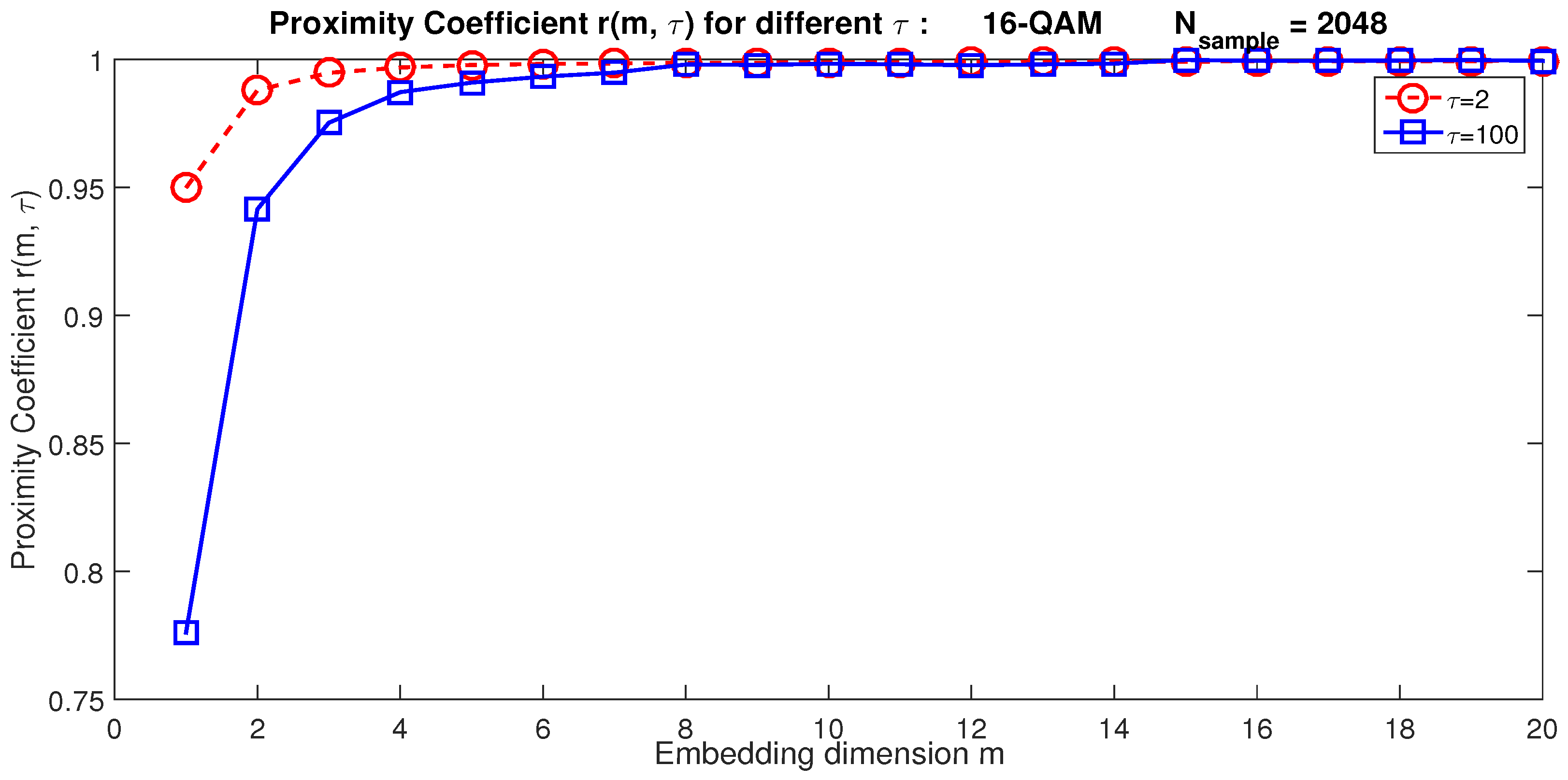
When m becomes greater than a limit value $m_{lim}$, the proximity coefficient $r(m,\tau )$ converges to one. Hence, $m_0=m_{lim}+1$ becomes the minimum embedding dimension [42]. Based on Equation (7), we can observe that $r(m,\tau )$ depends on the time delay value $\tau$. This assertion is corroborated by simulation results. Figure 1 illustrates, for example, the evolution of $r(m,\tau )$ for two extreme values of $\tau$; for $\tau =2$, the optimal value of $m_0=6$; whereas for $\tau =100$, we obtain $m_0=9$. As m depends on the choice of $\tau$, we propose hereinafter an optimization strategy to find simultaneously the optimal values of m and $\tau$.

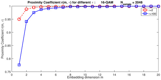
Figure 1. The proximity coefficient $r(m,\tau )$ based on the embedding dimension m for a 16-QAM signal.

3.1.3. Optimal Values of m and $\tau$

$r(m,\tau )$ is a bivariate function whose expression leads to

$$\underset{(m,\tau )\to (m_0,{\tau }_0)}{lim}r(m,\tau )=1$$

(8)

So we define the cost function $f(m,\tau )$:

$$f(m,\tau )=\overline{a}(m,\tau )-\overline{a}(m+1,\tau )$$

(9)

The optimal values $m_0$ and ${\tau }_0$ become

$$(m_0,{\tau }_0)=\underset{(m,\tau )\in {\mathbb{N}}^{*}}{argmin}\left\{f(m,\tau )\right\}$$

(10)

Numerical results show that values of $(m_0,{\tau }_0)$ obtained from (10) become independent from modulation schemes, SNR, and the number of samples per symbol $N_s$. Figure 2 illustrates the cost function f$(m,\tau )$ with respect to $(m,\tau )$ for a noisy 16-QAM signal. We can notice that

$$\begin{array}{c}\hfill \forall \tau \ge 6,m\ge 1,\mathbf{f}(m,\tau )\to 0\end{array}$$

(11)

The number K of state vectors is given by

$$K=N-(m-1)\tau \ge K_{min}$$

(12)

Based on Takens’ theorem (in Taken’s theorem, the phase space of a system can be reliably reconstructed if and only if $m\ge 2D+1$, where $D\ge 1$ is the dimension of the system attractor [36,44]) and the minimum number $K_{min}$ of state vectors for reliable detection, we conclude that $m_0$ and ${\tau }_0$ should be chosen in the following ranges:

$$\begin{array}{c}\hfill \left(m_0,{\tau }_0\right)\in \left[3;\frac{N-K_{min}}{{\tau }_0}\right]\times \left[6;\frac{N-K_{min}}{2}\right]\end{array}$$

(13)

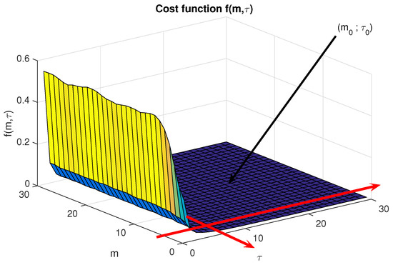
Figure 2. The cost function $\mathbf{f}(m,\tau )$ based on $(m,\tau )$: The flat area of the curve $\mathbf{f}(m,\tau )$ corresponds to a set of optimal values of $\left(m,\tau \right)$. Consequently, the optimal values $\left(m_0,{\tau }_0\right)$ of $\left(m,\tau \right)$ should be chosen as follows $\left(m_0,{\tau }_0\right)\subset \left[3;\frac{N}{{\tau }_0}\right]\times \left[6;\frac{N}{2}\right]$.

However, we notice that in practice $K_{min}\ll N$. Consequently, we can

$$\begin{array}{c}\hfill \left(m_0,{\tau }_0\right)\in \left[3;\frac{N}{{\tau }_0}\right]\times \left[6;\frac{N}{2}\right]\end{array}$$

(14)

The recurring states in the phase space can be highlighted by the Recurrence Plot.

3.2. Recurrence Plot

The Recurrence Plot (RP) illustrates recurrences contained in a signal. The RP is based on the recurrence matrix ${\mathbf{R}}_{i,j}^{(\epsilon ,m)}$ [30,36]:

$${\mathbf{R}}_{i,j}^{(\epsilon ,m)}=\Theta \left\{\epsilon -{∥{\mathbf{x}}_i-{\mathbf{x}}_j∥}_2\right\}$$

(15)

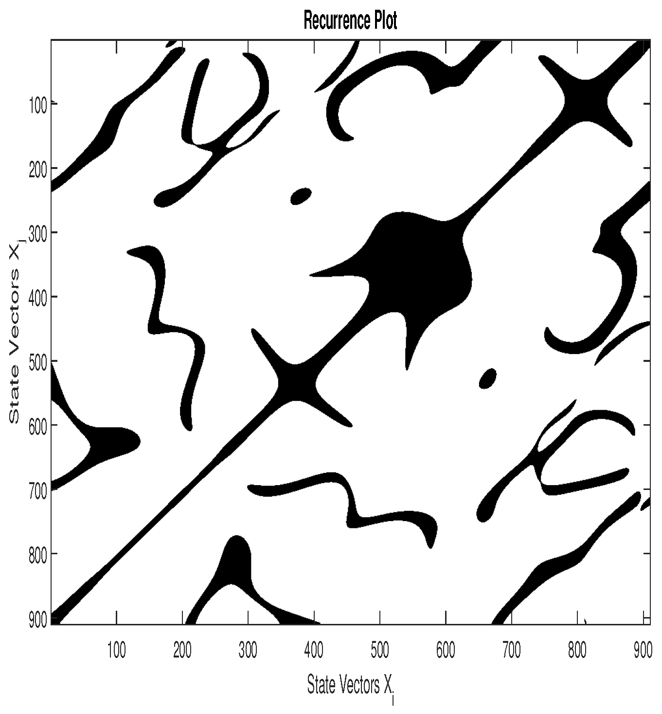
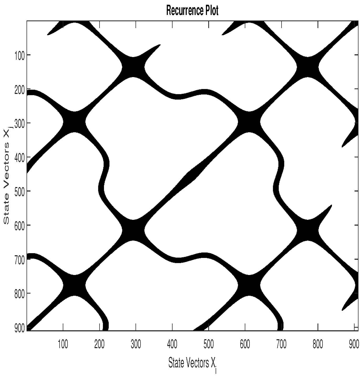
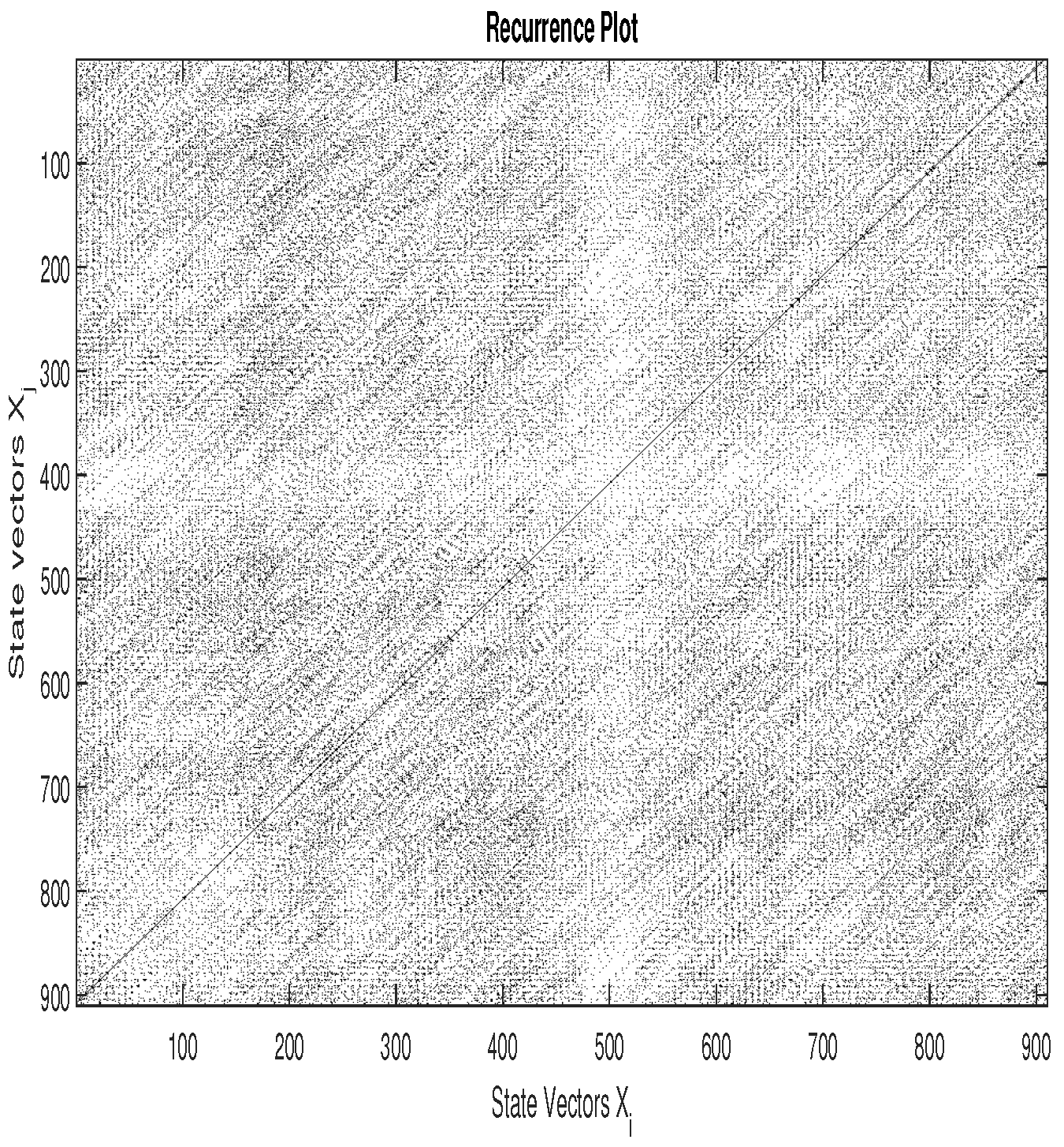
where $i,j\in \{1,\cdots ,K\}$ and $K=N-(m-1)\tau$ denotes the number of reconstructed state vectors ${\mathbf{x}}_k$; $\epsilon$ is the recurrence threshold, $\Theta (.)$ represents Heavisides’ step function, and ${∥.∥}_2$ is the $L_2$ or Frobenius norm. $d_{ij}={∥{\mathbf{x}}_i-{\mathbf{x}}_j∥}_2$ are the coefficients of the distance matrix M. According to Equation (15), the states ${\mathbf{x}}_i$ and ${\mathbf{x}}_j$ are recurring states if $∥{\mathbf{x}}_i-{\mathbf{x}}_j∥<\epsilon$. In the RP, a recurrence is represented by a black dot. If the parameters m, $\tau$, and $\epsilon$ are optimal, the RP presents some intrinsic patterns of the system. For example, Figure 3, Figure 4 and Figure 5 represent, respectively, the RP of 16-QAM signal, GMSK signal, and a random zero mean White Gaussian Noise (WGN) with a variance ${\sigma }_b^2$. We can notice that the patterns in the RP of the 16-QAM signal are different from those of the GMSK signal, whereas the RP of the WGN has no particular pattern. Heuristically, we can set the recurrence threshold as $\epsilon =0.5{\sigma }_y$ where ${\sigma }_y^2$ denotes the variance of the observed signal $y\left(n\right)$; the embedding parameters are established as $m=16$ and $\tau =6$.

Figure 3. RP according to Equation (15) of a 16-QAM signal.

Figure 4. RP of a Gaussian Minimum Shift Keying (GMSK) signal.

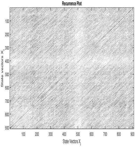
Figure 5. RP of White Gaussian Noise.

As the visual analysis of RP is not objective, Zbilut and Webber introduced a procedure to quantify RP structures [45,46]. In the literature, one has five classical tools to perform the RQA. Some RQA tools are based on the recurrence density, while others use the line structures of the RP [36]. The classical RQA tools are developed and extended in [30,36]. The main challenge with classical or extended RQA tools is the choice of an optimal recurrence threshold $\epsilon$ of Equation (15). A small value of $\epsilon$ does not reveal noticeable occurrences, while a large value of $\epsilon$ may lead to the appearance of neighbors for most of the existing points and cause false occurrences [30,47]. The choice of $\epsilon$ is a delicate issue affecting the reliability of the spectrum sensing based on classical or extended RQA tools [20]. To overcome this issue, we propose in the following sections a new algorithm called the Recurrence-Analysis-based Detector (RAD), which only exploits the distance matrix. This distance matrix does not depend on the recurrence threshold $\epsilon$ and nor does the proposed detection model RAD.

4. Recurrence-Analysis-Based Detector

The Recurrence Rate (RR) is an essential tool of RQA. Our previous works based on the RQA detection model [20] show that an RR-based detection model (RRD) suffers from major shortcomings, as follows:

• It cannot detect the presence of a communication signal when SNR $\le -5$ dB.
• It is very sensitive to the recurrence threshold $\epsilon$.
• The computational cost is relatively high.
• The performance of an RRD is sensitive to the types of modulations of a communication signal.

To overcome the above limitations, we develop hereinafter a new detection model, the Recurrence Analysis Detection model (RAD), which is able to operate in very low SNR conditions. In order to reduce drastically the computational cost and avoid the delicate issue of the recurrence threshold $\epsilon$, the RAD only uses the distances $d_{ij}={∥{\mathbf{x}}_i-{\mathbf{x}}_j∥}_2$ of the upper triangular part of the distance matrix.

4.1. Detection Model

Usually, the RQA is performed on the entire distance matrix $D={\left(d_{ij}\right)}_{1\le i,j\le K}$ of different state vectors. As D is a symmetrical matrix, in order to reduce the computational cost, we use the upper triangular part of D, without the main diagonal defined by its general coefficients:

$$D_{ij}=d_{ij};\forall 1\le i<j\le K$$

(16)

We denote by ${\mathbf{u}}_d$ the coefficients of the first upper diagonal of D and by ${\mathbf{u}}_{\Delta }$ the other coefficients of the upper triangular part of D, without the main diagonal. ${\mathbf{u}}_d$ and ${\mathbf{u}}_{\Delta }$ verify two great properties:

• For a WGN, ${\mathbf{u}}_d$ and ${\mathbf{u}}_{\Delta }$ have the same Probability Density Function (PDF), which is not the case for a noisy communication signal. Hence, to detect the presence of a communication signal, we check if ${\mathbf{u}}_d$ is representative of ${\mathbf{u}}_{\Delta }$. For this purpose, we use a statistical test of conformity to evaluate this representativeness [48].
• The ${\mathbf{u}}_d$ of a WGN or a communication signal has the same PDF. This remark allows us to design a detector free of noise variance estimation.

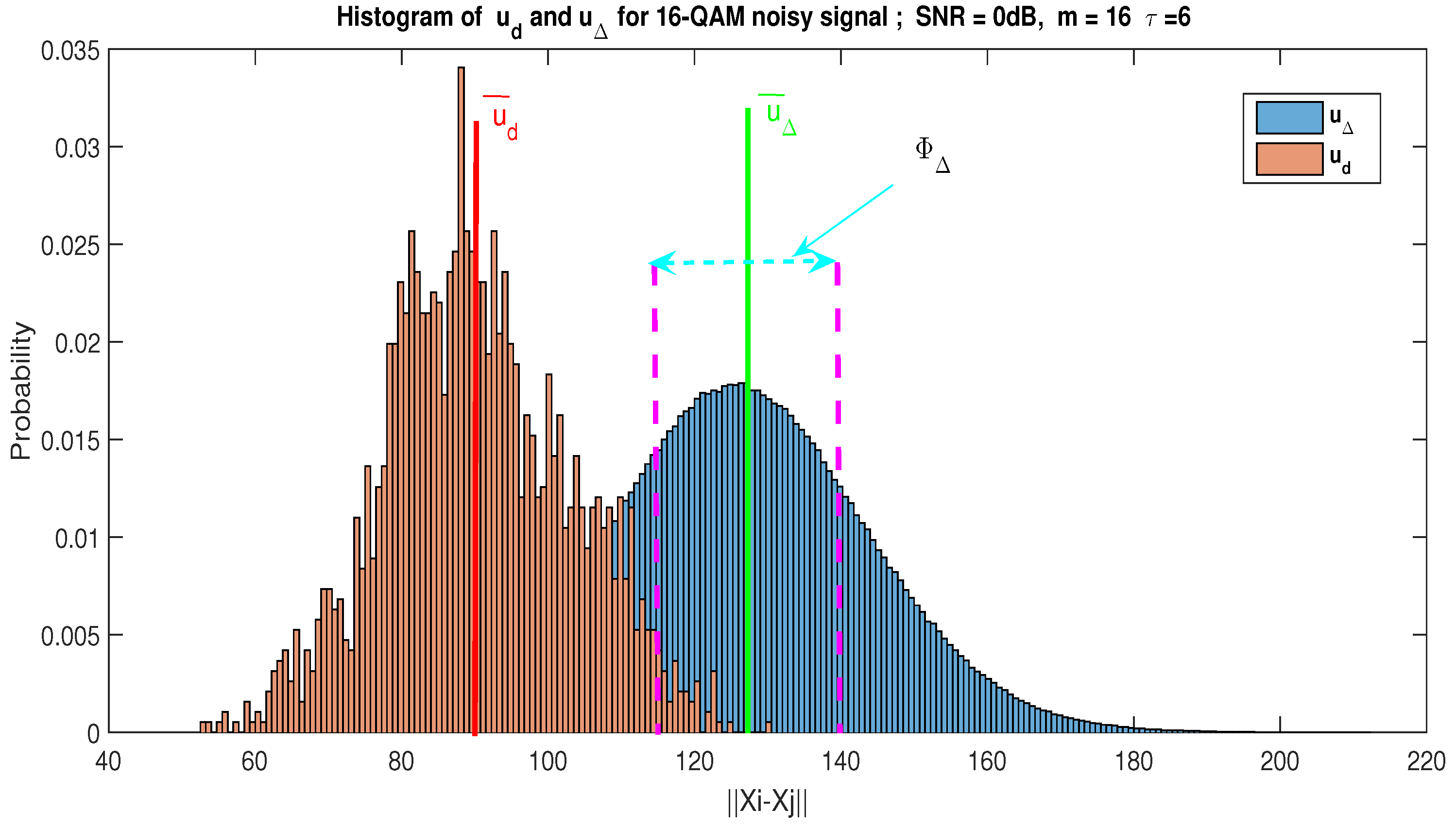
To provide a better understanding of this notion of representativeness, we present the histogram of the ${\mathbf{u}}_d$ and ${\mathbf{u}}_{\Delta }$ of WGN and the communication signal, respectively, in Figure 6 and Figure 7, and we define the confidence interval ${\Phi }_{\Delta }$ as follows:

$${\Phi }_{\Delta }=\left[{\overline{\mathbf{u}}}_{\Delta }-\lambda ;{\overline{\mathbf{u}}}_{\Delta }+\lambda \right]$$

(17)

where ${\overline{\mathbf{u}}}_{\Delta }$ is the average value of ${\mathbf{u}}_{\Delta }$ and $\lambda$ is the predetermined detection threshold for RAD. Further details about $\lambda$ can be found in Section 4.2.4.

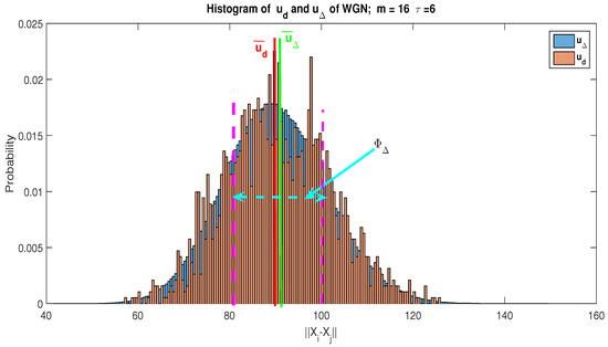
Figure 6. Histogram of ${\mathbf{u}}_d$ and ${\mathbf{u}}_{\Delta }$ for a White Gaussian Noise (WGN): We have ${\overline{u}}_d=90.6$ and ${\overline{u}}_{\Delta }=90$. For $P_{fa}=0.01$, the detection threshold of the RAD becomes $\lambda =12.5$. Based on the ${\overline{u}}_{\Delta }$ value, the confidence interval becomes ${\Phi }_{\Delta }=\left[77.5;102.5\right]$. We notice that ${\overline{u}}_d\in {\Phi }_{\Delta }$. Consequently, using the conformity test, we can conclude that ${\mathbf{u}}_d$ is representative of ${\mathbf{u}}_{\Delta }$.

Figure 7. Histogram of ${\mathbf{u}}_d$ and ${\mathbf{u}}_{\Delta }$ for a noisy 16-QAM signal; SNR = 0 dB. In this example, we have ${\overline{u}}_d=90$ and ${\overline{u}}_{\Delta }=127$. With $P_{fa}=0.01$, we obtain $\lambda =12.5$ and ${\Phi }_{\Delta }=\left[114.5;139.5\right]$. We notice that ${\mathbf{u}}_d$ is not representative of ${\mathbf{u}}_{\Delta }$, because ${\overline{u}}_d\notin {\Phi }_{\Delta }$.

On the basis of the histogram of distance and by using Kolmogorov–Smirnov test [49], for a WGN only, we note that ${\mathbf{u}}_d$ and ${\mathbf{u}}_{\Delta }$ can be approximated by the same PDF (see Figure 6). Consequently, by using the statistical test of conformity based on the estimation average value, we show that ${\mathbf{u}}_d$ is representative of ${\mathbf{u}}_{\Delta }$. Indeed, ${\overline{\mathbf{u}}}_d\in {\Phi }_{\Delta }$; ${\overline{\mathbf{u}}}_d$ denotes the average value of ${\mathbf{u}}_d$. Contrariwise, Figure 7 gives the histogram of distance for a communication signal buried in the WGN with an SNR $=0$ dB; we can notice that ${\overline{\mathbf{u}}}_d\notin {\Phi }_{\Delta }$, so ${\mathbf{u}}_d$ is not representative of ${\mathbf{u}}_{\Delta }$.

Using the statistical test of conformity, we propose the following test statistic T:

$$T=|{\overline{\mathbf{u}}}_{\Delta }-{\overline{\mathbf{u}}}_d|\stackrel{{\mathcal{H}}_1}{\underset{{\mathcal{H}}_0}{\gtrless }}\lambda$$

(18)

In the course of our work, we establish the analytical expressions of the probability of detection $P_d$ and the probability of false alarm $P_{fa}$ in order to compare the theoretical and experimental results.

4.2. Analytical Expression of the Probability of False Alarm

The probability of a false alarm $P_{fa}$ can be expressed from the PDF of T under ${\mathcal{H}}_0$. In order to find this PDF, one should evaluate the PDF of ${\overline{\mathbf{u}}}_{\Delta }$ and ${\overline{\mathbf{u}}}_d$; see Equation (18).

4.2.1. The PDF of ${\overline{\mathbf{u}}}_{\Delta }$ under Hypothesis ${\mathcal{H}}_0$

Under ${\mathcal{H}}_0$, the average value ${\overline{\mathbf{u}}}_{\Delta }$ of ${\mathbf{u}}_{\Delta }$ is defined as follows:

$${\overline{\mathbf{u}}}_{\Delta /{\mathcal{H}}_0}=\frac{1}{K_{\Delta }}\sum _{k=1}^{K_{\Delta }}{u}_{\Delta /{\mathcal{H}}_0}^{\left(k\right)}$$

(19)

where $K_{\Delta }=(K-1)(K/2-1)$ and $u_{\Delta /{\mathcal{H}}_0}^{\left(k\right)}\in \{d_{ij};1\le i\le K-2;i+2\le j\le K\}$.

Based on the central limit theorem for independent random variables and for a large K, ${\overline{\mathbf{u}}}_{\Delta /{\mathcal{H}}_0}$ is asymptotically normally distributed with mean ${\overline{\mathbf{u}}}_{\Delta /{\mathcal{H}}_0}$ and variance ${\sigma }_{\Delta /{\mathcal{H}}_0}^2$:

$${\overline{\mathbf{u}}}_{\Delta /{\mathcal{H}}_0}\mapsto \mathcal{N}\left({\mu }_{\Delta /{\mathcal{H}}_0},{\sigma }_{\Delta /{\mathcal{H}}_0}^2\right)$$

(20)

where

$$\begin{array}{c}\hfill {\mu }_{\Delta /{\mathcal{H}}_0}=\mathbb{E}\left[{\overline{\mathbf{u}}}_{\Delta /{\mathcal{H}}_0}\right]\end{array}$$

(21)

$$\begin{array}{c}\hfill {\sigma }_{\Delta }^2=var\left[{\overline{\mathbf{u}}}_{\Delta /{\mathcal{H}}_0}\right]\end{array}$$

(22)

To calculate ${\mu }_{\Delta /{\mathcal{H}}_0}$ and ${\sigma }_{\Delta /{\mathcal{H}}_0}^2$, we can use the PDF $f_{{\mathbf{u}}_{\Delta /{\mathcal{H}}_0}}$ (u) of ${\mathbf{u}}_{\Delta /{\mathcal{H}}_0}$. An outcome $u_{\Delta /{\mathcal{H}}_0}$ of ${\mathbf{u}}_{\Delta /{\mathcal{H}}_0}$ is given by

$$u_{\Delta /{\mathcal{H}}_0}=d_{ij}=\sqrt{\sum _{k=0}^{m-1}{\left(b_{i+k\tau }-b_{j+k\tau }\right)}^2}$$

(23)

As $b\left(n\right)\mapsto \mathcal{N}\left(0,{\sigma }_b^2\right)$, then $b_{i+k\tau }-b_{j+k\tau }\mapsto \mathcal{N}\left(0,2{\sigma }_b^2\right)$ and $v_k=\left(\frac{b_{i+k\tau }-b_{j+k\tau }}{{\sigma }_b\sqrt{2}}\right)\mapsto \mathcal{N}\left(0,1\right)$.

By setting $Z=\sqrt{{\sum }_{k=0}^{m-1}{v}_k^2}$, we can conclude that Z follows a Chi distribution $\chi \left(m\right)$ with m degrees of freedom [50,51]:

$$Z=\frac{{\mathbf{u}}_{\Delta /{\mathcal{H}}_0}}{{\sigma }_b\sqrt{2}}\mapsto \succ \left(m\right)$$

(24)

The expectation value $\mathbb{E}\left[Z\right]$ and variance $var\left[Z\right]$ of Z are given as follows [50,51]:

$$\begin{array}{c}\hfill \mathbb{E}\left[Z\right]={\mu }_Z=\sqrt{2}\frac{\Gamma \left(\frac{m+1}{2}\right)}{\Gamma \left(\frac{m}{2}\right)}\end{array}$$

(25)

$$\begin{array}{c}\hfill var\left[Z\right]=m-{\mu }_Z^2\end{array}$$

(26)

where $\Gamma \left(m\right)={\int }_0^{+\infty }{x}^{m-1}{e}^{-x}dx$ is the Gamma function.

From Equation (24), we show that the PDF $f_{{\mathbf{u}}_{\Delta /{\mathcal{H}}_0}}$ of ${\mathbf{u}}_{\Delta /{\mathcal{H}}_0}$ is defined as follows: [52]:

$$f_{{\mathbf{u}}_{\Delta /{\mathcal{H}}_0}}\left(u\right)=\frac{u^{m-1}}{2^{m-1}{\sigma }_b^m\Gamma \left(\frac{m}{2}\right)}exp\left[-\frac{u^2}{4{\sigma }_b^2}\right]$$

(27)

The mean ${\mu }_{\Delta /{\mathcal{H}}_0}$ and variance ${\sigma }_{\Delta /{\mathcal{H}}_0}^2$ of ${\overline{X}}_{\Delta /{\mathcal{H}}_0}$ can be determined by using Equation (24) as follows:

$$\begin{array}{c}\hfill {\mu }_{\Delta /{\mathcal{H}}_0}={\sigma }_b\sqrt{2}\mathbb{E}\left[Z\right]\end{array}$$

(28)

$$\begin{array}{c}\hfill {\sigma }_{\Delta /{\mathcal{H}}_0}^2=\frac{2{\sigma }_b^2}{K_{\Delta }}var\left[Z\right]\end{array}$$

(29)

Finally, we have ${\overline{\mathbf{u}}}_{\Delta /{\mathcal{H}}_0}\mapsto \mathcal{N}\left({\mu }_{\Delta /{\mathcal{H}}_0},{\sigma }_{\Delta /{\mathcal{H}}_0}^2\right)$ with

$$\begin{array}{c}\hfill {\mu }_{\Delta /{\mathcal{H}}_0}=2{\sigma }_b\frac{\Gamma \left(\frac{m+1}{2}\right)}{\Gamma \left(\frac{m}{2}\right)}\end{array}$$

(30)

$$\begin{array}{c}\hfill {\sigma }_{\Delta /{\mathcal{H}}_0}^2=\frac{2{\sigma }_b^2}{K_{\Delta }}\left[m-2{\left(\frac{\Gamma \left(\frac{m+1}{2}\right)}{\Gamma \left(\frac{m}{2}\right)}\right)}^2\right]\end{array}$$

(31)

4.2.2. The PDF of ${\overline{\mathbf{u}}}_d$ under Hypothesis ${\mathcal{H}}_0$

Under ${\mathcal{H}}_0$, the average value ${\overline{\mathbf{u}}}_d$ of ${\mathbf{u}}_d$ is defined as follows:

$${\overline{\mathbf{u}}}_{d/{\mathcal{H}}_0}=\frac{1}{K_d}\sum _{k=1}^{K_d}{u}_{d_k/{\mathcal{H}}_0}^{\left(k\right)}$$

(32)

where $u_{d/{\mathcal{H}}_0}^{\left(k\right)}\in \left\{d_{i,i+1}\right\};1\le i\le K_d=K-1$.

Because of the structure of the upper triangular distance matrix, the coefficients of the first top diagonal $u_{d/{\mathcal{H}}_0}^{\left(k\right)}$ are strongly decorrelated. In addition, $K_d$ is a large number. Thus, we can approximate ${\overline{\mathbf{u}}}_d$ by a Gaussian variable by using the central limit theorem:

$${\overline{\mathbf{u}}}_{d/{\mathcal{H}}_0}\mapsto \mathcal{N}\left({\mu }_{d/{\mathcal{H}}_0},{\sigma }_{d/{\mathcal{H}}_0}^2\right)$$

(33)

Using a similar approach to the calculation of the expectation value ${\mu }_{\Delta /{\mathcal{H}}_0}$ and variance ${\sigma }_{\Delta /{\mathcal{H}}_0}^2$ of ${\overline{\mathbf{u}}}_{\Delta /{\mathcal{H}}_0}$, we obtain

$$\begin{array}{c}\hfill {\mu }_{d/{\mathcal{H}}_0}=2{\sigma }_b\frac{\Gamma \left(\frac{m+1}{2}\right)}{\Gamma \left(\frac{m}{2}\right)}\end{array}$$

(34)

$$\begin{array}{c}\hfill {\sigma }_{d/{\mathcal{H}}_0}^2=\frac{2{\sigma }_b^2}{K_d}\left[m-2{\left(\frac{\Gamma \left(\frac{m+1}{2}\right)}{\Gamma \left(\frac{m}{2}\right)}\right)}^2\right]\end{array}$$

(35)

4.2.3. The Probability Density Function of T under hypothesis ${\mathcal{H}}_0$

${\overline{\mathbf{u}}}_{d/{\mathcal{H}}_0}$ and ${\overline{\mathbf{u}}}_{\Delta /{\mathcal{H}}_0}$ are Gaussian random variables. Based on Equations (20), (30), (31) and (33)–(35) we end up with

$$\begin{array}{c}\hfill {\overline{\mathbf{u}}}_{\Delta /{\mathcal{H}}_0}-{\overline{\mathbf{u}}}_{d/{\mathcal{H}}_0}\mapsto \mathcal{N}\left(0,{\sigma }_0^2\right)\end{array}$$

(36)

where

$$\begin{array}{c}\hfill {\sigma }_0^2={\sigma }_{\Delta /{\mathcal{H}}_0}^2+{\sigma }_{d/{\mathcal{H}}_0}^2-2Cov\left({\overline{\mathbf{u}}}_{d/{\mathcal{H}}_0},{\overline{\mathbf{u}}}_{\Delta /{\mathcal{H}}_0}\right)\end{array}$$

(37)

Applying the random variable transformation theorem [52,53] on T from Equation (18), we end up with $t\ge 0$:

$$\begin{array}{c}\hfill f_{T/{\mathcal{H}}_0}\left(t\right)=\frac{2}{{\sigma }_0\sqrt{2\pi }}exp\left[-\frac{t^2}{2{\sigma }_0^2}\right]\end{array}$$

(38)

4.2.4. Probability of False Alarm and Detection Threshold

Based on Equation (38), the $P_{fa}$ is expressed as follows:

$$\begin{array}{c}\hfill P_{fa}={\int }_{\lambda }^{\infty }{f}_{T/{\mathcal{H}}_0}\left(t\right)dt=erfc\left(\frac{\lambda }{{\sigma }_0\sqrt{2}}\right)\end{array}$$

(39)

$erfc\left(x\right)$ denotes the Complementary Error Function—the Complementary Error Function $erfc\left(x\right)$ is defined as follows:

$$erfc\left(x\right)=\frac{2}{\sqrt{\pi }}{\int }_x^{+\infty }{e}^{-{\theta }^2}d\theta$$

—and the detection threshold $\lambda$ is

$$\begin{array}{c}\hfill \lambda ={\sigma }_0\sqrt{2}erf{c}^{-1}\left(P_{fa}\right)\end{array}$$

(40)

4.3. Analytical Expression of the Probability of Detection

Taking into account the presence of the communication signal $s\left(n\right)$ and keeping the same approach as under $H_0$, we demonstrate that

$$\begin{array}{c}\hfill {\overline{\mathbf{u}}}_{\Delta /H_1}\mapsto \mathcal{N}\left({\mu }_{\Delta /H_1},{\sigma }_{\Delta /H_1}^2\right)\end{array}$$

(41)

$$\begin{array}{c}\hfill {\overline{\mathbf{u}}}_{d/H_1}\mapsto \mathcal{N}\left({\mu }_{d/H_1},{\sigma }_{d/H_1}^2\right)\end{array}$$

(42)

where

$$\begin{array}{c}\hfill {\mu }_{\Delta /H_1}=2\sqrt{{\sigma }_s^2+{\sigma }_b^2}\frac{\Gamma \left(\frac{m+1}{2}\right)}{\Gamma \left(\frac{m}{2}\right)}\end{array}$$

(43)

$$\begin{array}{c}\hfill {\sigma }_{\Delta /H_1}^2=\frac{2({\sigma }_s^2+{\sigma }_b^2)}{K_{\Delta }}\left[m-2{\left(\frac{\Gamma \left(\frac{m+1}{2}\right)}{\Gamma \left(\frac{m}{2}\right)}\right)}^2\right]\end{array}$$

(44)

$$\begin{array}{c}\hfill {\mu }_{d/H_1}=2{\sigma }_b\frac{\Gamma \left(\frac{m+1}{2}\right)}{\Gamma \left(\frac{m}{2}\right)}\end{array}$$

(45)

$$\begin{array}{c}\hfill {\sigma }_{d/H_1}^2=\frac{2{\sigma }_b^2}{K_d}\left[m-2{\left(\frac{\Gamma \left(\frac{m+1}{2}\right)}{\Gamma \left(\frac{m}{2}\right)}\right)}^2\right]\end{array}$$

(46)

We deduce the PDF of T under the hypothesis $H_1$ as follows:

$$\begin{array}{c}\hfill f_{T/H_1}\left(t\right)=\frac{1}{{\sigma }_1\sqrt{2\pi }}\left[e^{-{\left(\frac{t-{\mu }_1}{{\sigma }_1\sqrt{2}}\right)}^2}+e^{-{\left(\frac{t+{\mu }_1}{{\sigma }_1\sqrt{2}}\right)}^2}\right]\end{array}$$

(47)

with $t\ge 0$. ${\mu }_1$ and ${\sigma }_1^2$ are given by

$$\begin{array}{c}\hfill {\mu }_1={\mu }_{\Delta /H_1}-{\mu }_{d/H_1},\end{array}$$

(48)

$$\begin{array}{c}\hfill {\sigma }_1^2={\sigma }_{\Delta /H_1}^2+{\sigma }_{d/H_1}^2-2Cov\left({\overline{\mathbf{u}}}_{\Delta /H_1},{\overline{\mathbf{u}}}_{d/H_1}\right)\end{array}$$

(49)

Consequently, the Probability of Detection $P_d$ becomes

$$\begin{array}{c}\hfill \begin{array}{cc}\hfill P_d& ={\int }_{\lambda }^{+\infty }{f}_{T/H_1}\left(t\right)dt\hfill \\ & =1-\frac{1}{2}\left[erfc\left(\frac{-\lambda -{\mu }_1}{{\sigma }_1\sqrt{2}}\right)-erfc\left(\frac{\lambda -{\mu }_1}{{\sigma }_1\sqrt{2}}\right)\right]\hfill \end{array}\end{array}$$

(50)

5. Simulations Results

To evaluate the efficiency and the robustness of the proposed detection method, we generate Receiver Operating Characteristic (ROC) curves using Monte Carlo simulations [54,55]. The parameters defined in Table 1 are used with different kinds of communication signals, such as 64-QAM, 16-QAM, BPSK, and 4-ASK.

Table 1. Simulation parameters.

Entity	Parameters	Value
PU’s signal	Sampling frequency $F_e$	128 kHz
	Symbol rate	16 Bd
	Bandwidth of Interest B	24 kHz
SU’s Detector	Observation time	15.6 ms
	Sampling Frequency	128 KHz
Embedding parameters	Dimension m	16
	time delay $\tau$	6
Transmission Channel	Noise Model	AWGN

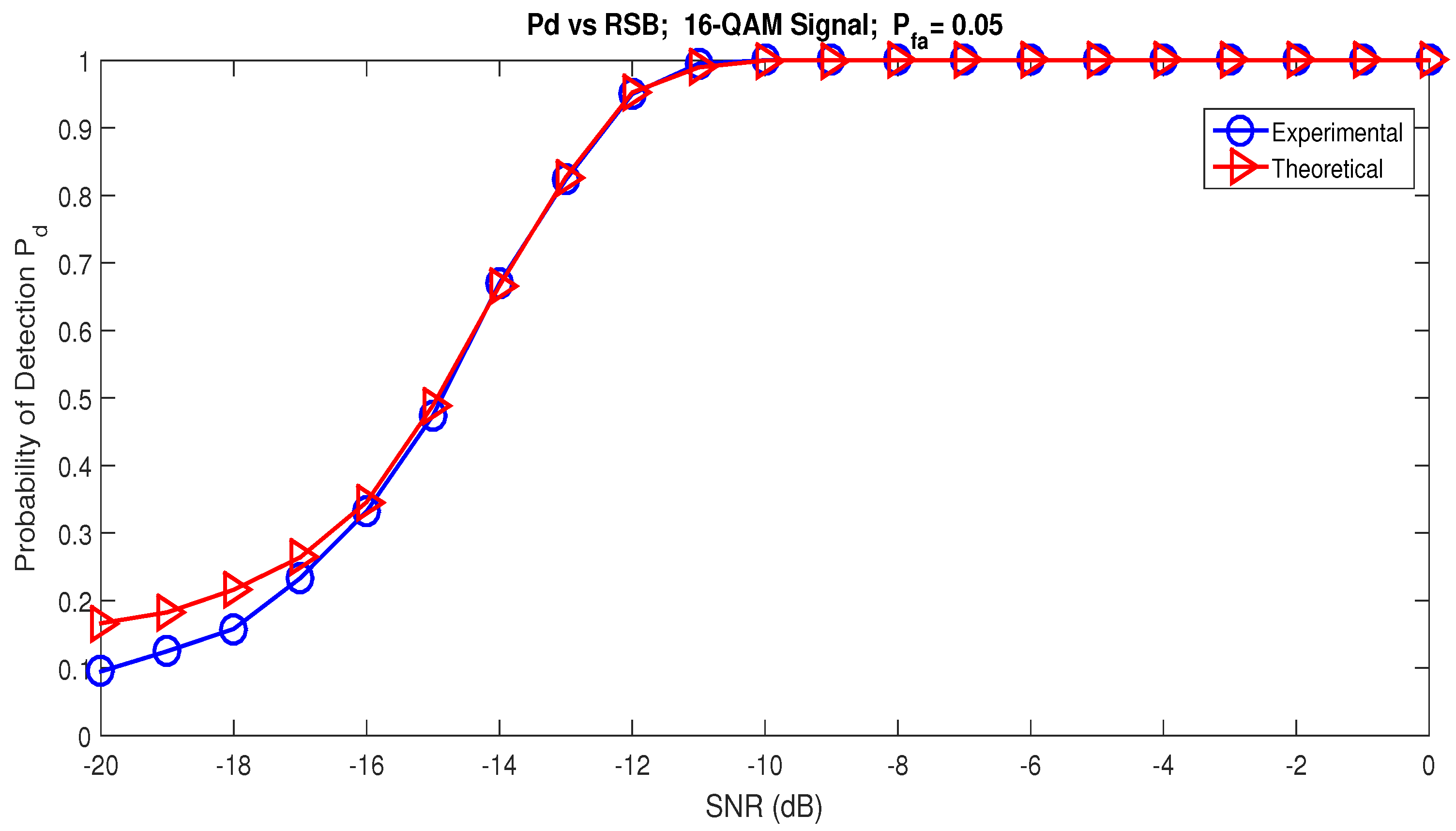
In order to compare the theoretical and experimental performance of the RAD, we generated $P_d$ versus SNR performance curves. Figure 8 shows these performance curves. The theoretical curves were generated by Equation (50) and the experimental curves according to the Monte Carlo simulations. It can be clearly observed that the theoretical results match the simulated ones. From the theoretical and experimental curves, reliable detection is possible as soon as $\mathrm{SNR}\ge -12$ dB with $P_d\ge 0.95$ and $P_{fa}=0.05$.

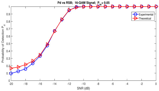
Figure 8. Theoretical and experimental probability of detection for RAD versus SNR.

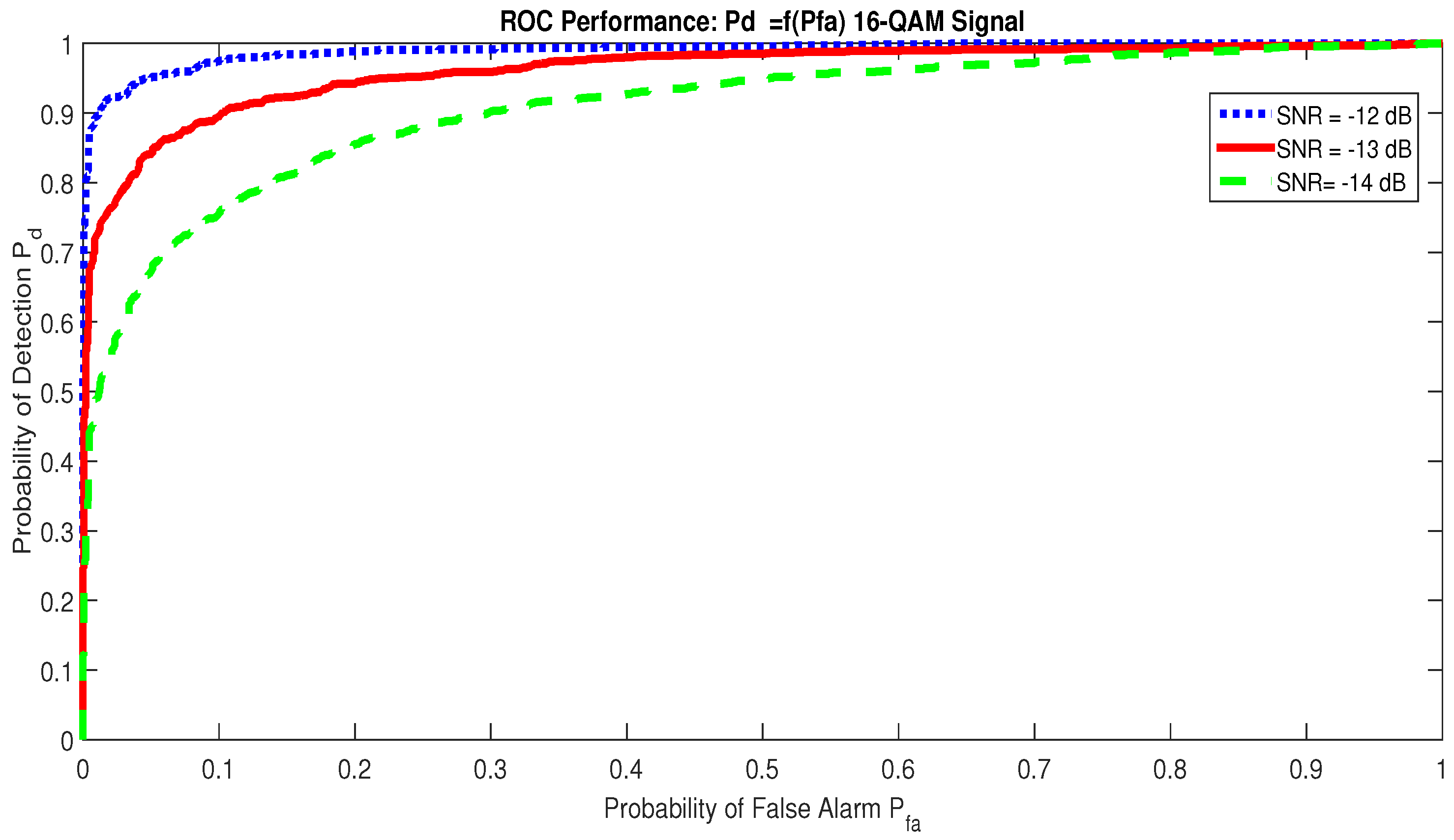
The Receiver Operating Characteristic curves for different $\mathrm{SNR}$ values can be viewed in Figure 9. Here, the RAD is applied on a 16-QAM signal, and the observation time is $31.25$ ms. For SNR $=-14$ dB and $P_{fa}=0.1$, the RAD detects the presence of a communication signal with $P_d=0.76$, but for SNR $=-13$ dB, $P_d=0.9$. The detector proves itself powerful as soon as the SNR $\ge -12$ dB, since the detection probability $P_d=0.95$ with a very low value of $P_{fa}=0.05$; see Figure 9.

Figure 9. Receiver Operating Characteristic for $16-QAM$ signal.

Another advantage of the proposed detector is its robustness against any type of classical modulations, such as QAM, PSK, and ASK; see Figure 10, where the ROC curves for 4-ASK, BPSK, and 64-QAM signal are almost identical.

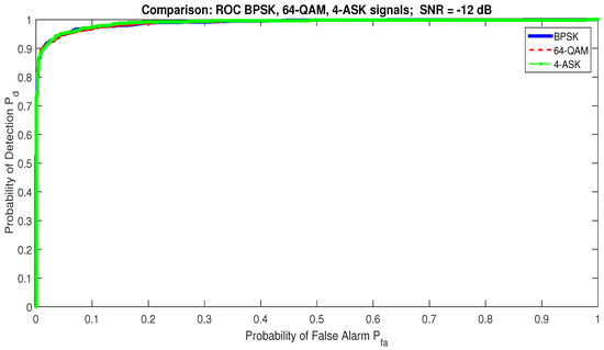
Figure 10. Robust RQA detector insensitivity versus classical modulation techniques.

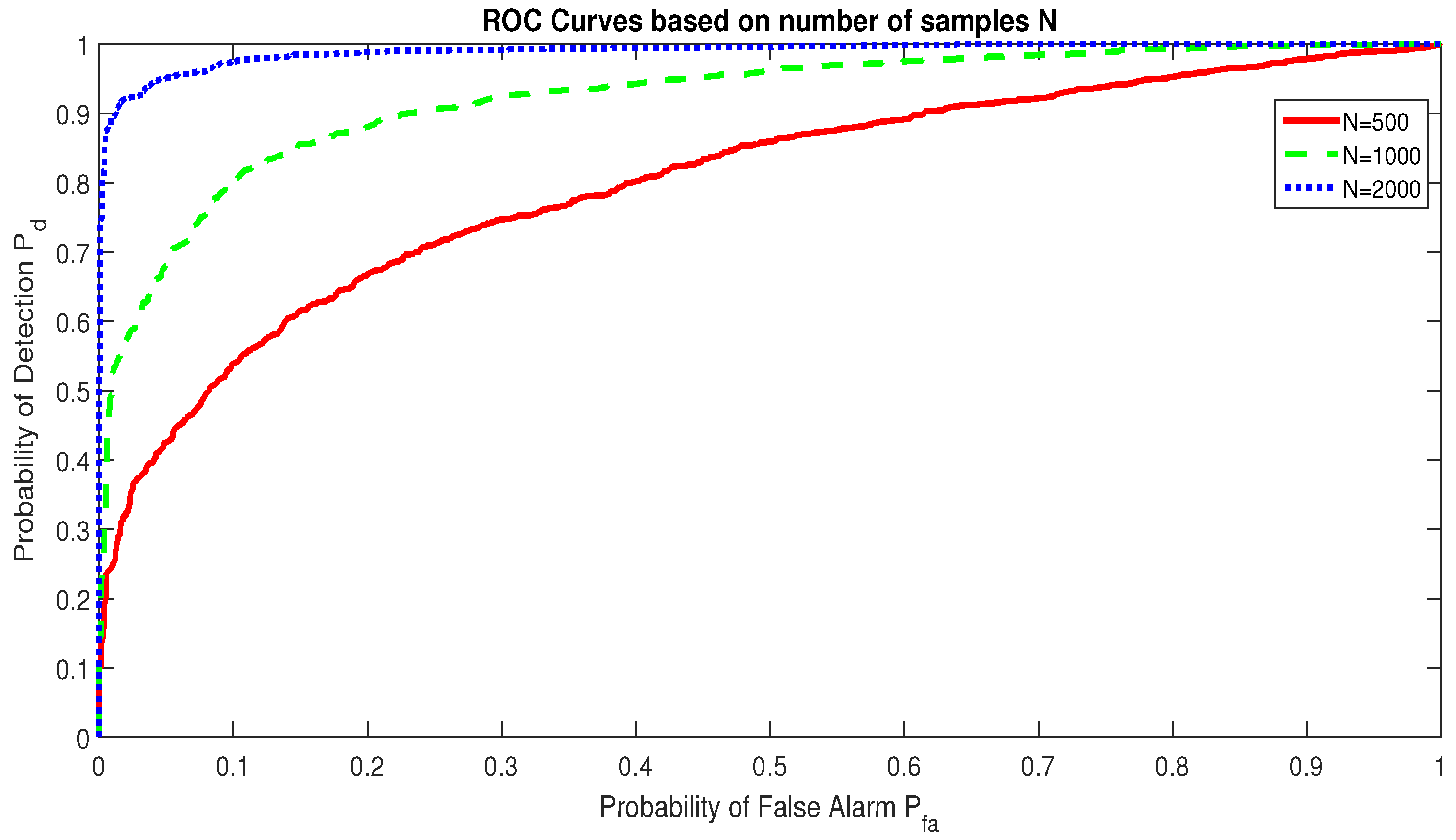
The performance of RAD increases with the number of samples N. Figure 11 depicts this performance evolution based on N in a Gaussian channel where SNR $=-12$ dB. We notice that for $P_{fa}=0.1$, the RAD detects the communication signal with $P_d=0.5$ when $N=500$ samples, with $P_d=0.8$ when $N=1000$ samples, and with $P_d=0.97$ when $N=2000$ samples.

Figure 11. Receiver Operating Characteristic of the RAD model based on the number of observed samples in a Gaussian channel with $\mathrm{SNR}=-12$ dB.

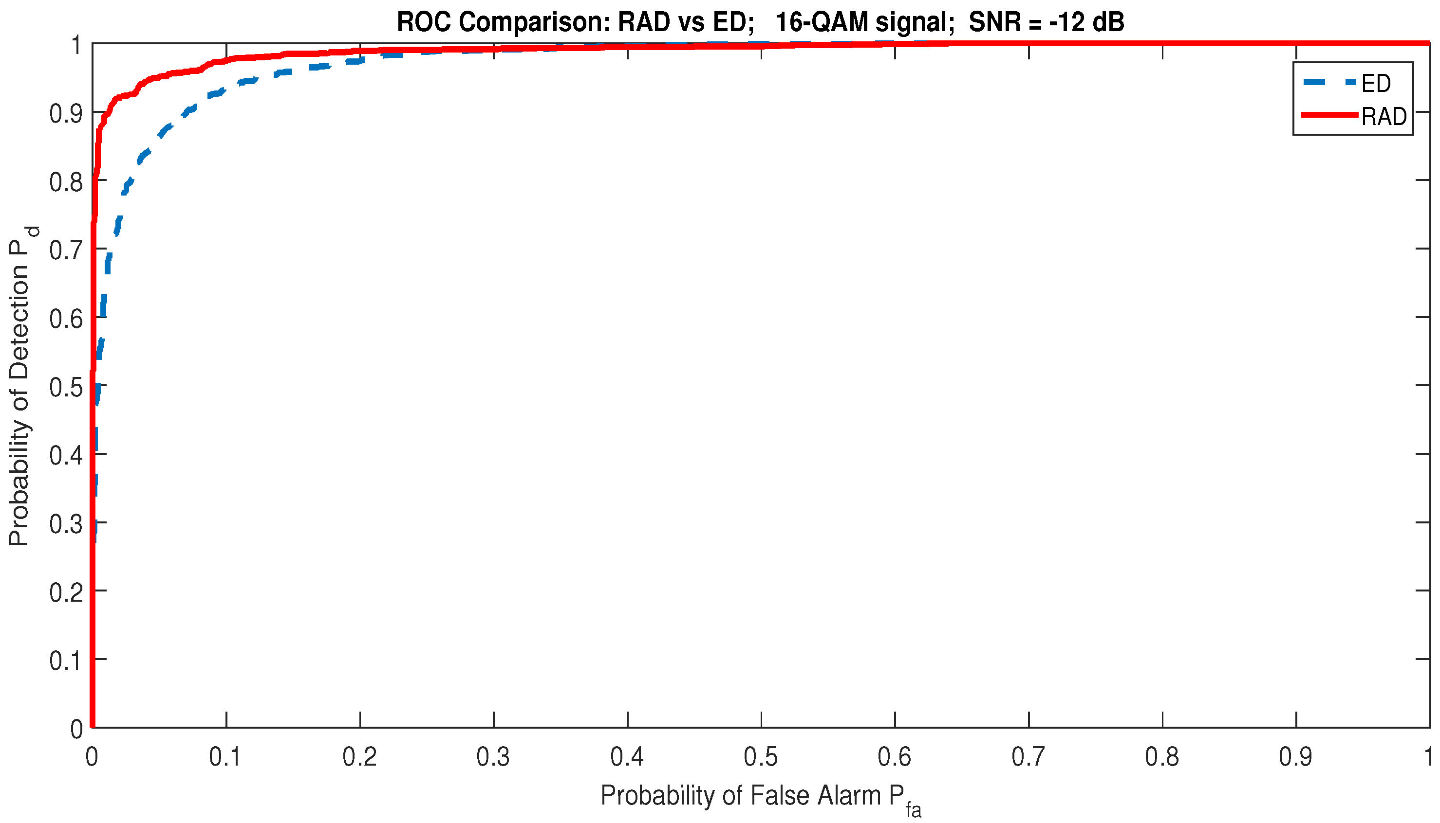
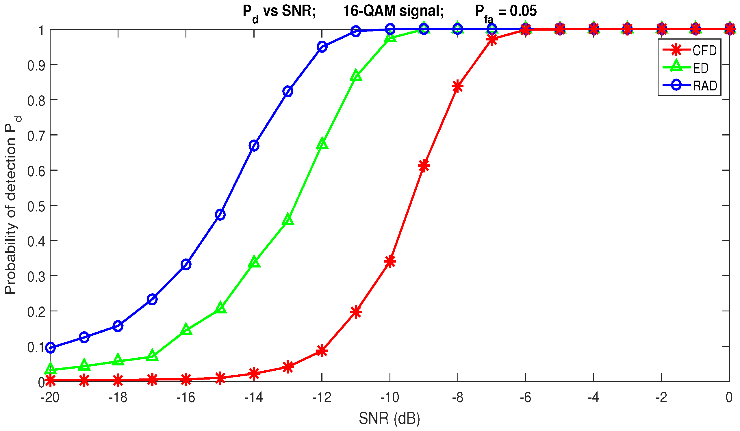
By comparing RAD with two other blind spectrum sensing algorithms, Energy Detection (ED) [56] and Cyclostationary Features Detector (CFD) [57,58], and according to the results presented in Figure 12 and Figure 13, we notice the superiority of the RAD to ED and CFD in a Gaussian channel. For example, for the $\mathrm{SNR}=-12$ dB and $P_{fa}=0.05$, the RAD detects the signal with $P_d=0.95$, whereas the probability of detection for the ED is only $P_d=0.67$ (see Figure 12). Figure 13 shows that the RAD is able to detect the communication signal in very weak low SNR conditions. For $-12$ dB ≤ SNR $\le -10$ dB, the RAD detects the presence of a communication signal with $P_d\ge 0.95$ for $P_{fa}=0.05$. ED achieves RAD performance only when SNR $\ge -10$ dB, and CFD works correctly when SNR $\ge -7$ dB with $P_d\ge 0.97$.

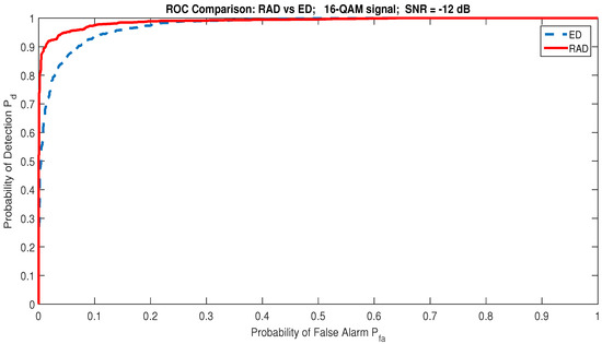
Figure 12. ROC performance: ED vs RAD. The RAD is superior to ED.

Figure 13. Comparison of Energy Detector (ED), Cyclostationary Features Detector (CFD), and Recurrence Analysis Detector (RAD).

After testing the performance of the detector in a Gaussian channel, we are now interested in the behavior of the RAD in a multipath channel. As a model, we use model D of the Rayleigh channel defined in [59] with the following parameters (Table 2 and Table 3):

Table 2. Rayleigh Channel Model Features.

Model D of Rayleigh Channel
Entity	Parameters	Value
Features	Number of Path	6
	Doppler Frequency $f_{d_{max}}$	1.2 kHz

Table 3. Delay and Gain values for 6 paths [59].

Path Number	1	2	3	4	5	6
Delay (ns)	0	300	8900	12,900	17,100	20,000
Gain (dB)	0	−2.5	−12.8	−10.0	−25.2	−16.0

Figure 14 summarizes the performance of the RAD in a noisy Rayleigh channel. The RAD’s performance remains almost unchanged. It detects a communication signal with $P_d\ge 0.92$ with $P_{fa}=0.05$ as soon as SNR $\ge -12$ dB.

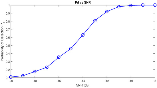
Figure 14. Performance Curve $P_d$ as a function of SNR for 16-QAM signal in a Rayleigh channel.

6. Complexity Analysis of Recurrence-Analysis-Based Detector

Theoretical and experimental analyses show the superiority of the RAD compared with the Energy Detector (ED) and the Cyclostationary Feature Detector (CFD) in a low SNR scenario detection process. The complexity of the algorithms is measured through the number of complex multiplications that the algorithms have to perform for the calculation of the test statistics [60]. In this section, we provide the complexity analyses of the ED, CFD, and RAD.

6.1. Complexity Analysis of Energy-Based Detector

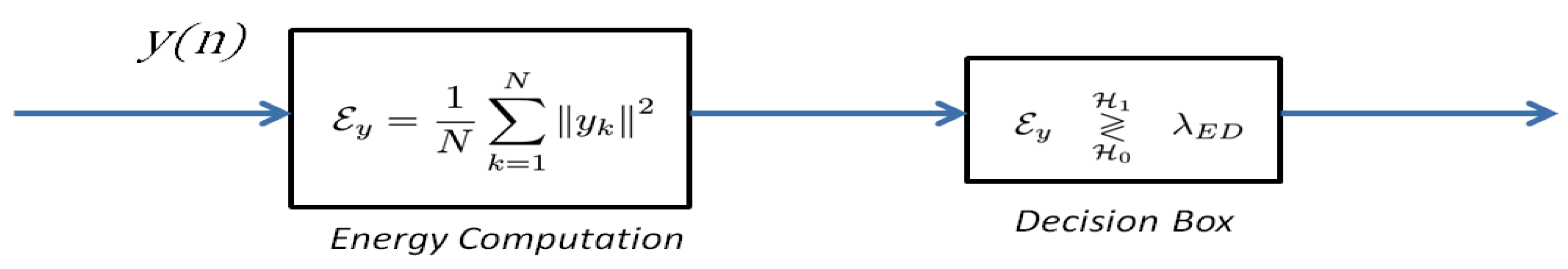
Let $y\left(n\right)$ be the observed signal with N samples $y_k$. The energy ${\mathcal{E}}_y$ of $y\left(n\right)$ is given by

$${\mathcal{E}}_y=\frac{1}{N}\sum _{k=1}^N{y}_k^2$$

(51)

The ED detection process is summarized in Figure 15.

Figure 15. Energy Detector process. ${\lambda }_{ED}$ denotes the detection threshold of the ED.

The complexity of the computation can be evaluated according to Equation (51). N multiplication operations are required to perform $y_k^2$. Consequently, the computation complexity $C_{ED}$ becomes [60]

$$C_{ED}=N$$

(52)

6.2. Complexity Analysis of Cyclostationary-Feature-Based Detector

In a blind context, the CFD is based on the reliable estimation of the cyclic spectrum [13,61,62]. The crest factor $F_c$ of the cyclic spectrum can be used as a decision statistic [13]:

$$F_c\left(\alpha \right)=\frac{{max}_{\alpha }D\left(\alpha \right)}{\sqrt{\frac{1}{2N+1}{\sum }_{k=1}^{2N+1}{D}^2\left(\alpha \right)}}\stackrel{{\mathcal{H}}_1}{\underset{{\mathcal{H}}_0}{\gtrless }}{\lambda }_{CFD}$$

(53)

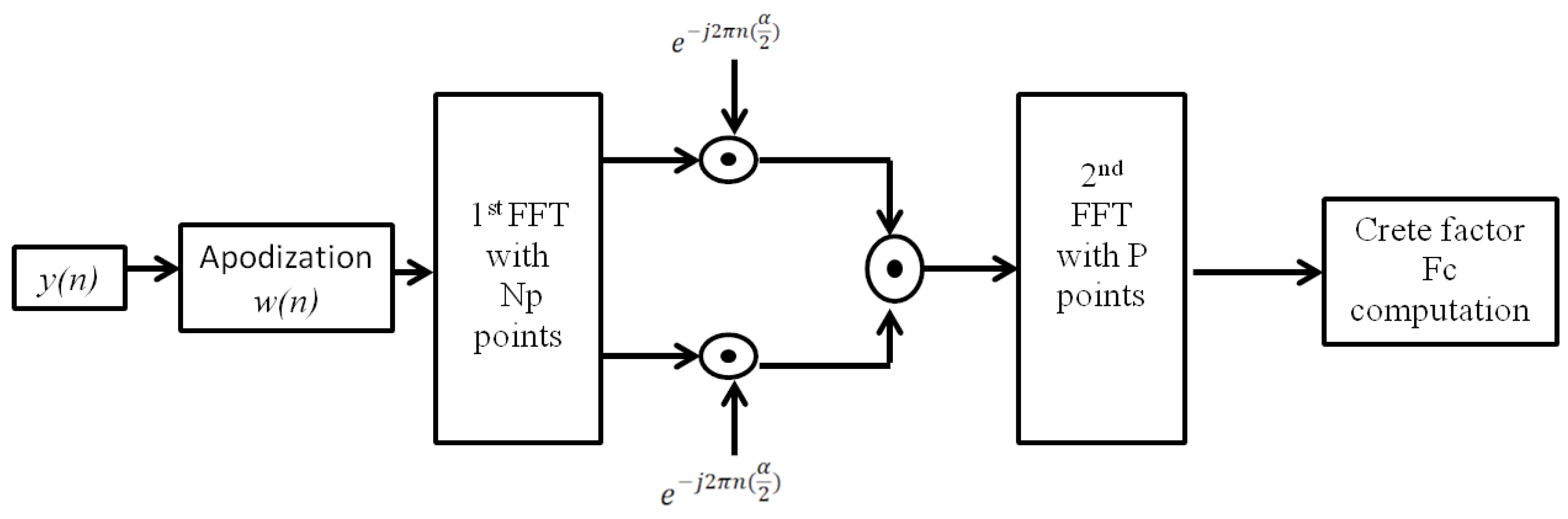
where $\alpha$ stands for the cyclic frequency and $D\left(\alpha \right)$ denotes the Cyclic Domain Profile (CDP). The computation of $F_c$ requires six steps [13]. First, a Hamming sliding window $w\left(n\right)$ is used to apodize the observed signal $y\left(n\right)$. Then, we apply a first Fast Fourier Transform (FFT) and calculate the complex demodulates of the apodized signal. After that, we compute the spectral correlation of the different complex demodulates and apply a second FFT. At the end, we obtain the cyclic spectrum, and we compute the crest factor $F_c$ of the cyclic spectrum.

Let N be the number of samples contained in the observed signal $y\left(n\right)$ and $N_p$ be the number of samples contained in each apodized block of $y\left(n\right)$. $L=\frac{N_p}{4}$ denotes the decimation factor, and $P=\frac{N}{L}$ is the number of apodized blocks from $y\left(n\right)$. The apodization is carried out with a Hamming window [13,61,63]. Figure 16 summarizes the essential steps of $F_c$ computation.

Figure 16. Different steps of the CFD detection process.

The apodization equation is defined as follows:

$$r_k=w_k{y}_k;k=1..N_p$$

(54)

where $w_k$ denotes the Hamming window coefficients, $y_k$ is the samples of the observed signal $y\left(n\right)$, and $r_k$ becomes the coefficients resulting from the apodization.

The apodization step requires $P{N}_p$ multiplication operations. The second step in the CFD detection process is the first FFT applied on apodized blocks. The complexity of FFT computation is known as $N_p{log}_2{N}_p$. Consequently, the P apodized blocks require $P{N}_{p}lo{g}_2{N}_p$ multiplication operations. The complex demodulates computation requires $P{N}_p^2$ multiplication operations, and the step of complex demodulates multiplication requires $P^2{N}_p^2$ multiplication operations.

The second FFT with P data points to obtain the estimation of cyclic spectrum requires $N_p^{2}P{log}_{2}P$ multiplication operation and the calculation of crest factor $F_c$ alone requires $2N+1$ multiplication operations.

Finally, the algorithmic complexity of CFD, $C_{CFD}$, is

$$C_{CFD}=34N^2+64NL+10N+2$$

(55)

6.3. Algorithmic Complexity of Recurrence-Analysis-Based Detector

To make decisions, the RAD uses a statistic test defined in Equation (18). The RAD detection process is summarized in Figure 17.

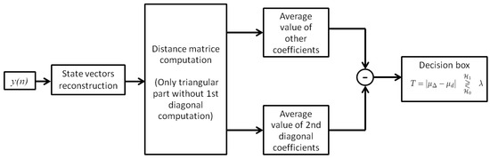
Figure 17. Different steps of the RAD detection process.

The algorithmic complexity of the RAD essentially concerns the distance matrix computation and the calculation of average values of distance matrix coefficients. From the observed signal $y\left(n\right)$ containing N samples, we obtain $K=N-(m-1)\tau$ state vectors. Each state vector contains m coordinates. The distance $d_{ij}=∥{\mathbf{x}}_{-}{\mathbf{x}}_j∥$ from the state vector ${\mathbf{x}}_i$ to other state vectors ${\mathbf{x}}_j$ requires $mK$ addition operations. Because we exploit only the upper triangular part of the distance matrix with the main diagonal coefficients, we use $\frac{m}{2}K(K-2)$ addition operations. The computation of the average value of the first upper diagonal requires K elementary operations, and the average value of other coefficients requires $\frac{{(K-2)}^2}{2}$ elementary operations. The statistic test of the RAD requires one addition operation. Consequently, the computation complexity $C_{RAD}$ of the RAD becomes

$$\begin{array}{c}\hfill C_{RAD}=2N^2+4N(\tau -m\tau -1)+\left[2{\left(m\tau \right)}^2+2{\tau }^2-4m{\tau }^2-4\tau +2m\tau +6\right]\end{array}$$

(56)

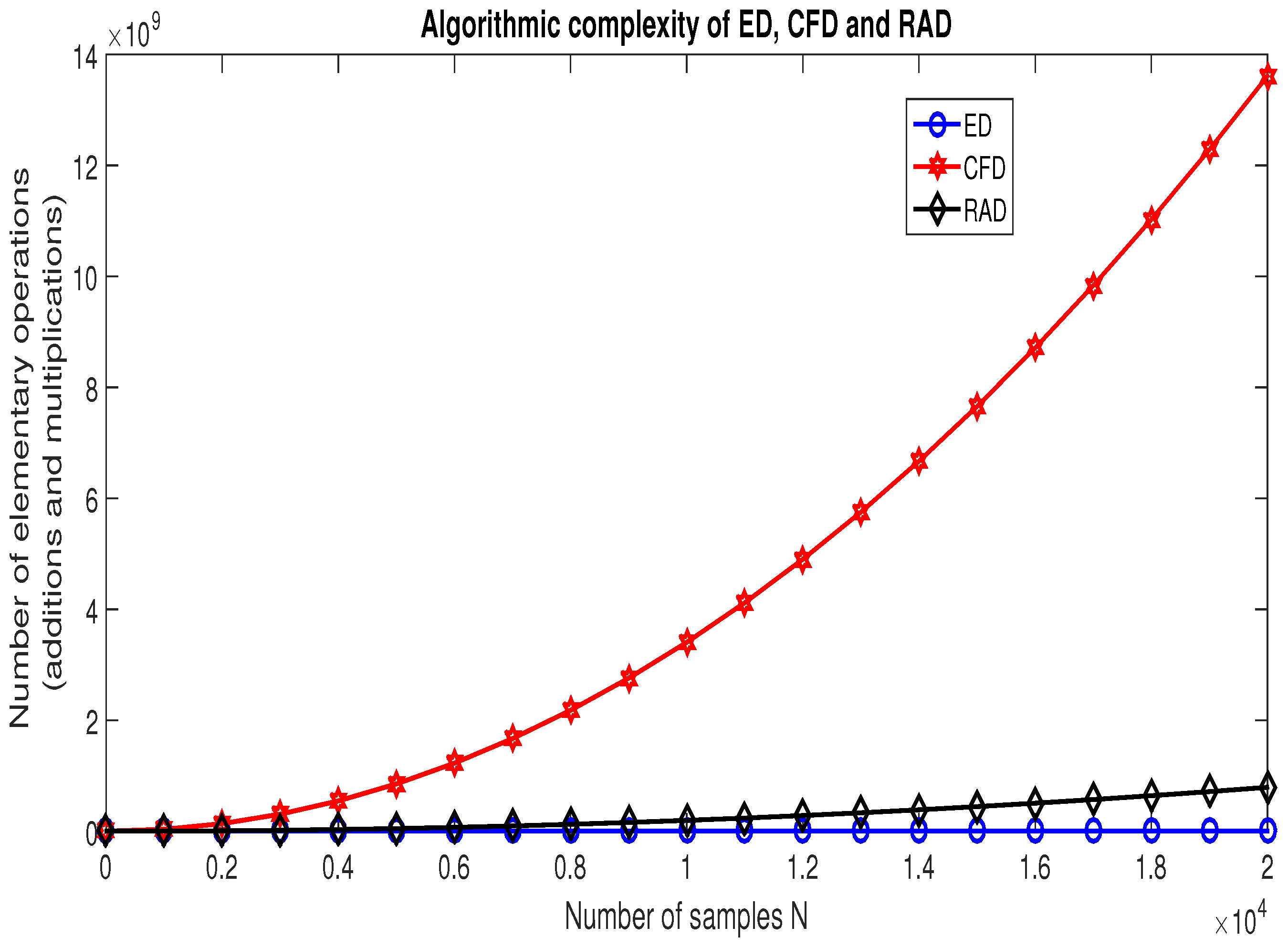
From Equations (52), (55), and (56), in Figure 18, we generated the curves of the evolution of the algorithmic complexity of the ED, CFD, and RAD based on the number of samples contained in the observed signal $y\left(n\right)$. The results in Figure 18 show that ED is the simplest algorithm, whereas CFD is the most complicated one. We also notice that the RAD algorithm is less complicated than the CFD algorithm.

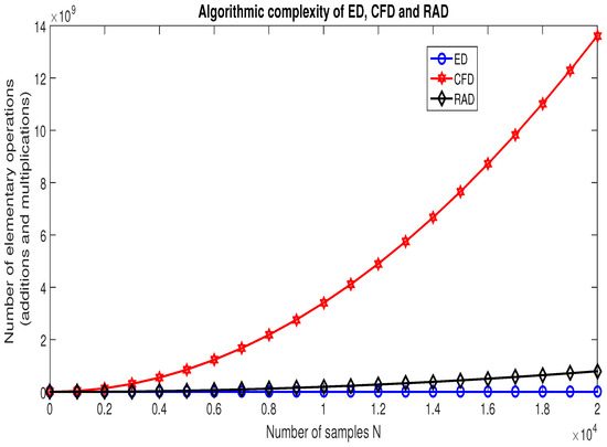
Figure 18. Curves of the algorithmic complexity of ED, CFD, and RAD.

7. Conclusions

This paper deals with the problem of noncooperative spectrum sensing in very low SNR conditions. Many algorithms have recently been developed to overcome the scarcity of radio spectrum. However, most of them suffer from noise uncertainty and do not work correctly in very low SNR conditions. In this paper, we use the promising approach of the Recurrence Quantification Analysis (RQA) to propose a robust detection model, named the Recurrence-Analysis-based Detector (RAD). The RAD benefits from the exploitation of the similitude among the different state vectors. Indeed, our analyses reveal that for a White Gaussian Noise, the coefficients contained on the first upper diagonal are representative of other coefficients of the distance matrix, which is not the case for a communication signal. Thus, by applying a conformity test between the coefficients of the first upper diagonal and other coefficients of the distance matrix, the presence or absence of a communication signal can be revealed. The RAD presents five major advantages: it is more robust than the Energy Detector (ED) and the Cyclostationary Feature Detector (CFD), which are widely used in the noncooperative spectrum sensing context; it does not suffer from noise variance estimation, because the estimation of the noise variance is not required during the spectrum sensing process; it is able to detect the communication signal in a very low SNR condition; contrary to the ED, the RAD is able to distinguish a noisy communication signal and a high energy noise; the RAD does not need a high computational cost like the CFD. Our present work also presents two major contributions. First, we determined, for digital communication signals, the optimal values of the time delay $\tau$ and embedding dimension m needed for the phase space reconstruction. Second, we established the analytical expression of detection threshold $\lambda$, the probability of detection $P_d$, and the probability of false alarm $P_{fa}$ of the detection model based on RQA. From the ROC curves, we can notice without ambiguity that the RAD is more robust than the ED and CFD algorithms. Our current simulations show that the RAD is able to detect the communication signal for SNR ≥ −12 dB. In addition to facilitating the blind detection of communication signals, RQA could be used to accurately estimate the characteristic frequencies of the signal of interest. In our future work, we will optimize the performance of the RAD detector based on this reliable estimation of the characteristic frequencies of the signal of interest.

References

- Haykin, S. Cognitive radio: Brain-empowered wireless communications. IEEE J. Sel. Areas Commun. 2005, 23, 201–220. [Google Scholar] [CrossRef]
- Mansour, A.; Mesleh, R.; Abaza, M. New challenges in wireless and free space optical communications. Opt. Lasers Eng. 2017, 89, 95–108. [Google Scholar] [CrossRef]
- Nasser, A.; Mansour, A.; Yao, K.C.; Chaitou, M.; Charara, H. Spatial and time diversities for canonical correlation significance test in spectrum sensing. In Proceedings of the Signal Processing Conference (EUSIPCO), 2016 24th European, Budapest, Hungary, 29 August–2 September 2016; pp. 1232–1236. [Google Scholar]
- Nasser, A.; Mansour, A.; Yao, K.C.; Charara, H.; Chaitou, M. Spectrum sensing for full-duplex cognitive radio systems. In Proceedings of the International Conference on Cognitive Radio Oriented Wireless Networks (CROWNCOM), Grenoble, France, 30 May–1 June 2016; Springer: Cham, Switzerland, 2016; pp. 363–374. [Google Scholar]
- Nasser, A.; Mansour, A.; Yao, K.; Abdallah, H.; Charara, H. Spectrum sensing based on cumulative power spectral density. EURASIP J. Adv. Signal Process. 2017, 1, 38–56. [Google Scholar] [CrossRef]
- Moawad, A.; Yao, K.; Mansour, A.; Gautier, R. Autocepstrum Approach for Spectrum Sensing in Cognitive Radio. In Proceedings of the 2018 15th International Symposium on Wireless Communication Systems (ISWCS), Lisbon, Portugal, 28–31 August 2018; pp. 1–6. [Google Scholar]
- Ding, G.; Wang, J.; Wu, Q.; Zhang, L.; Zou, Y.; Yao, Y.; Chen, Y. Robust Spectrum Sensing With Crowd Sensors. IEEE Trans. Commun. 2014, 62, 3129–3143. [Google Scholar] [CrossRef]
- Luo, L.; Roy, S. Efficient Spectrum Sensing for Cognitive Radio Networks via Joint Optimization of Sensing Threshold and Duration. IEEE Trans. Commun. 2012, 60, 2851–2860. [Google Scholar] [CrossRef]
- Zeng, Y.; Liang, Y. Eigenvalue-based spectrum sensing algorithms for cognitive radio. IEEE Trans. Commun. 2009, 57, 1784–1793. [Google Scholar] [CrossRef]
- Li, B.; Li, S.; Nallanathan, A.; Nan, Y.; Zhao, C.; Zhou, Z. Deep Sensing for Next-Generation Dynamic Spectrum Sharing: More Than Detecting the Occupancy State of Primary Spectrum. IEEE Trans. Commun. 2015, 63, 2442–2457. [Google Scholar] [CrossRef]
- Burel, G.; Bouder, C.; Berder, O. Detection of direct sequence spread spectrum transmissions without prior knowledge. In Proceedings of the GLOBECOM’01, IEEE Global Telecommunications Conference, San Antonio, TX, USA, 25–29 November 2001; Volume 1, pp. 236–239. [Google Scholar]
- Zhang, X.; Gao, F.; Chai, R.; Jiang, T. Matched filter based spectrum sensing when primary user has multiple power levels. China Commun. 2015, 12, 21–31. [Google Scholar] [CrossRef]
- Kadjo, J.M.; Yao, K.C.; Mansour, A. Blind detection of cyclostationary features in the context of Cognitive Radio. In Proceedings of the IEEE International Symposium on Signal Processing and Information Technology (ISSPIT), Limassol, Cyprus, 12–14 December 2016; pp. 150–155. [Google Scholar]
- Sobron, I.; Diniz, P.S.R.; Martins, W.A.; Velez, M. Energy Detection Technique for Adaptive Spectrum Sensing. IEEE Trans. Commun. 2015, 63, 617–627. [Google Scholar] [CrossRef]
- Lopez-Benitez, M.; Casadevall, F. Signal Uncertainty in Spectrum Sensing for Cognitive Radio. IEEE Trans. Commun. 2013, 61, 1231–1241. [Google Scholar] [CrossRef]
- Yang, K.; Huang, Z.; Wang, X.; Li, X. A Blind Spectrum Sensing Method Based on Deep Learning. Sensors 2019, 19, 2270. [Google Scholar] [CrossRef]
- Xue, H.; Gao, F. A machine learning based spectrum-sensing algorithm using sample covariance matrix. In Proceedings of the 2015 10th International Conference on Communications and Networking in China (ChinaCom), Shanghai, China, 15–17 August 2015; pp. 476–480. [Google Scholar]
- Zhang, K.; Li, J.; Gao, F. Machine learning techniques for spectrum sensing when primary user has multiple transmit powers. In Proceedings of the 2014 IEEE International Conference on Communication Systems, Macau, China, 19–21 November 2014; pp. 137–141. [Google Scholar]
- Xiao, H.; Zhou, X.; Tian, Y. Research on Wireless Spectrum Sensing Technology Based on Machine Learning. In Proceedings of the International Conference on Security, Privacy and Anonymity in Computation, Communication and Storage; Springer: Berlin/Heidelberg, Germany, 2018; pp. 472–479. [Google Scholar]
- Kadjo, J.M.; Yao, K.C.; Mansour, A. Blind Spectrum Sensing Based on Recurrence Quantification Analysis in the Context of Cognitive Radio. In Proceedings of the 26th European Signal Processing Conference (EUSIPCO), Rome, Italy, 3–7 September 2018; pp. 1835–1839. [Google Scholar]
- Ünal, B. Stability Analysis of Bitcoin using Recurrence Quantification Analysis. Chaos Theory Appl. 2022, 4, 104–110. [Google Scholar] [CrossRef]
- Martín, C.J.; Itayetzin, B.C.V.; Gertrudis, H.G.G.; Claudia, L. Nonlinear Dynamics of Heart Rate Variability after Acutely Induced Myocardial Ischemia by Percutaneous Transluminal Coronary Angioplasty. Entropy 2023, 25, 469. [Google Scholar] [CrossRef]
- Costa, D.G.d.B.; Reis, B.M.d.F.; Zou, Y.; Quiles, M.G.; Macau, E.E. Recurrence density enhanced complex networks for nonlinear time series analysis. Int. J. Bifurc. Chaos 2018, 28, 1850008. [Google Scholar] [CrossRef]
- Zhang, Q.; Chen, X.; Yin, F.; Hong, F. Analysis and Research on Chaotic Dynamics of Evaporation Duct Height Time Series with Multiple Time Scales. Atmosphere 2022, 13, 2072. [Google Scholar] [CrossRef]
- Marwan, N.; Kurths, J. Cross recurrence plots and their applications. In Mathematical Physics Research at the Cutting Edge; Nova Science Publishers: Hauppauge, NY, USA, 2004; pp. 101–139. [Google Scholar]
- Atapattu, S.; Tellambura, C.; Jiang, H. Energy Detection for Spectrum Sensing in Cognitive Radio; Springer: New York, NY, USA, 2014. [Google Scholar]
- Mitola, J.; Maguire, G.Q. Cognitive radio: Making software radios more personal. IEEE Pers. Commun. 1999, 6, 13–18. [Google Scholar] [CrossRef]
- Mitola, J. Cognitive Radio Architecture Evolution. Proc. IEEE 2009, 97, 626–641. [Google Scholar] [CrossRef]
- Naraghi-Pour, M.; Ikuma, T. Autocorrelation-Based Spectrum Sensing for Cognitive Radios. IEEE Trans. Veh. Technol. 2010, 59, 718–733. [Google Scholar] [CrossRef]
- Marwan, N.; Romano, M.C.; Thiel, M.; Kurths, J. Recurrence plots for the analysis of complex systems. Phys. Rep. 2007, 438, 237–329. [Google Scholar] [CrossRef]
- Webber, C.L., Jr.; Zbilut, J.P. Recurrence quantification analysis of nonlinear dynamical systems. Tutor. Contemp. Nonlinear Methods Behav. Sci. 2005, 94, 26–94. [Google Scholar]
- Anishchenko, V.S.; Astakhov, V.; Neiman, A.; Vadivasova, T.; Schimansky-Geier, L. Nonlinear Dynamics of Chaotic and Stochastic Systems: Tutorial and Modern Developments; Springer: Berlin/Heidelberg, Germany, 2007. [Google Scholar]
- Williams, G. Chaos Theory Tamed; Routledge: London, UK, 2014. [Google Scholar] [CrossRef]
- Ivancevic, V.G.; Ivancevic, T.T. Complex Nonlinearity: Chaos, Phase Transitions, Topology Change and Path Integrals; Springer: Berlin/Heidelberg, Germany, 2008. [Google Scholar]
- Kantz, H.; Schreiber, T. Nonlinear Time Series Analysis; Cambridge University Press: Cambridge, UK, 2004; Volume 7. [Google Scholar]
- Marwan, C.W.N. Mathematical and Computational Foundations of Recurrence Quantifications. In Recurrence Quantification Analysis. Understanding Complex Systems; Springer: Cham, Switzerland; AIP Publishing: Melville, NY, USA, 2015. Available online: https://ouci.dntb.gov.ua/en/works/leGrnZW7/ (accessed on 17 June 2024).
- Bradley, E.; Kantz, H. Nonlinear time-series analysis revisited. Chaos Interdiscip. J. Nonlinear Sci. 2015, 25, 097610. [Google Scholar] [CrossRef]
- Chelidze, D. Reliable Estimation of Minimum Embedding Dimension Through Statistical Analysis of Nearest Neighbors. J. Comput. Nonlinear Dyn. 2017, 12, 051024. [Google Scholar] [CrossRef]
- Kraskov, A.; Stögbauer, H.; Grassberger, P. Estimating mutual information. Phys. Rev. E 2004, 69, 066138. [Google Scholar] [CrossRef]
- Fraser, A.M.; Swinney, H.L. Independent coordinates for strange attractors from mutual information. Phys. Rev. A 1986, 33, 1134. [Google Scholar] [CrossRef]
- David, C.; Joseph, P.C. Experimental Nonlinear Dynamics Notes for MCE 567; Cambridge University Press: New York, NY, USA, 2000. [Google Scholar]
- Cao, L. Practical method for determining the minimum embedding dimension of a scalar time series. Phys. D Nonlinear Phenom. 1997, 110, 43–50. [Google Scholar] [CrossRef]
- Kennel, M.B.; Brown, R.; Abarbanel, H.D.I. Determining embedding dimension for phase-space reconstruction using a geometrical construction. Phys. Rev. A 1992, 45, 3403–3411. [Google Scholar] [CrossRef]
- Takens, F. Detecting strange attractors in turbulence. In Dynamical Systems and Turbulence, Warwick 1980; Springer: Berlin/Heidelberg, Germany, 1981; pp. 366–381. [Google Scholar]
- Webber, C.L., Jr.; Zbilut, J.P. Dynamical assessment of physiological systems and states using recurrence plot strategies. J. Appl. Physiol. 1994, 76, 965–973. [Google Scholar] [CrossRef]
- Zbilut, J.P.; Webber, C.L., Jr. Recurrence quantification analysis: Introduction and historical context. Int. J. Bifurc. Chaos 2007, 17, 3477–3481. [Google Scholar] [CrossRef]
- Thiel, M.; Romano, M.C.; Kurths, J.; Meucci, R.; Allaria, E.; Arecchi, F.T. Influence of observational noise on the recurrence quantification analysis. Phys. D Nonlinear Phenom. 2002, 171, 138–152. [Google Scholar] [CrossRef]
- Mansour, A. Probabilités et Statistiques pour les Ingénieurs: Cours, Exercices et Programmation; Hermes Science: Paris, France, 2007. [Google Scholar]
- Shorack, G.R.; Wellner, J.A. Empirical Processes with Applications to Statistics; SIAM: University City, PA, USA, 2009. [Google Scholar]
- Gooch, J.W. Encyclopedic Dictionary of Polymers; Springer: New York, NY, USA, 2010. [Google Scholar]
- Abell, M.L.; Braselton, J.P.; Rafter, J.A.; Rafter, J.A. Statistics with Mathematica; Academic Press: San Diego, CA, USA, 1999. [Google Scholar]
- Papoulis, A.; Pillai, S.U. Probability, Random Variables, and Stochastic Processes; McGraw-Hill Education: New York, NY, USA, 2002. [Google Scholar]
- Miller, S.; Childers, D. Probability and Random Processes: With Applications to Signal Processing and Communications; Academic Press: Cambridge, MA, USA, 2012. [Google Scholar]
- Kha, Q.H.; Ho, Q.T.; Le, N.Q.K. Identifying SNARE Proteins Using an Alignment-Free Method Based on Multiscan Convolutional Neural Network and PSSM Profiles. J. Chem. Inf. Model. 2022, 62, 4820–4826. [Google Scholar] [CrossRef]
- Nasser, A. Spectrum Sensing for Half and Full-Duplex Interwave Cognitive Radio System. Ph.D. Thesis, Université de Bretagne Occidentale, Brest, France, 2017. [Google Scholar]
- Chin, W.L.; Li, J.M.; Chen, H.H. Low-complexity energy detection for spectrum sensing with random arrivals of primary users. IEEE Trans. Veh. Technol. 2015, 65, 947–952. [Google Scholar] [CrossRef]
- Cohen, D.; Eldar, Y.C. Sub-Nyquist cyclostationary detection for cognitive radio. IEEE Trans. Signal Process. 2017, 65, 3004–3019. [Google Scholar] [CrossRef]
- Tani, A.; Fantacci, R.; Marabissi, D. A low-complexity cyclostationary spectrum sensing for interference avoidance in femtocell LTE-A-based networks. IEEE Trans. Veh. Technol. 2015, 65, 2747–2753. [Google Scholar] [CrossRef]
- Ahmadi, S.; Srinivasan, R.M.; Cho, H.; Park, J.; Cho, J.; Park, D. Channel Models for IEEE 802.16 m Evaluation Methodology Document; IEEE 802.16 Broadband Wireless Access Working Group, 2007; pp. 3–12. Available online: https://standards.ieee.org/ieee/802.16g/3635/ (accessed on 17 June 2024).
- Zayen, B.; Guibène, W.; Hayar, A. Performance comparison for low complexity blind sensing techniques in cognitive radio systems. In Proceedings of the 2010 2nd International Workshop on Cognitive Information Processing, Elba Island, Italy, 14–16 June 2010; pp. 328–332. [Google Scholar] [CrossRef]
- Gardner, W. Cyclostationarty in Communications and Signal Processing; IEEE PRESS: New York, NY, USA, 1994. [Google Scholar]
- Gardner, W. The spectral correlation theory of Cyclostationary time-series. Signal Process. 1986, 11, 13–36. [Google Scholar] [CrossRef]
- Gardner, W. Exploitation Of Spectral Redundancy In Cyclostationary Signals. IEEE Signal Process. Mag. 1991, 8, 14–36. [Google Scholar] [CrossRef]
Disclaimer/Publisher’s Note: The statements, opinions and data contained in all publications are solely those of the individual author(s) and contributor(s) and not of MDPI and/or the editor(s). MDPI and/or the editor(s) disclaim responsibility for any injury to people or property resulting from any ideas, methods, instructions or products referred to in the content. |
© 2024 by the authors. Licensee MDPI, Basel, Switzerland. This article is an open access article distributed under the terms and conditions of the Creative Commons Attribution (CC BY) license (https://creativecommons.org/licenses/by/4.0/).