Wavelet-Based Estimation of Damping from Multi-Sensor, Multi-Impact Data

Abstract

Accurate damping estimation is crucial for structural health monitoring and machinery diagnostics. This article introduces a novel wavelet-based framework for extracting the damping ratio from multiple impulse responses of vibrating systems. Extracting damping ratios is a numerically sensitive task, further complicated by the common assumption in the literature that impacts are perfectly aligned—a condition rarely met in practice. To address the challenge of non-synchronized recordings, we propose two wavelet-based algorithms that leverage wavelet energy for improved alignment and averaging in the wavelet domain to reduce noise, enhancing the robustness of damping estimation. Our approach provides a fresh perspective on the application of wavelets in damping estimation. We conduct a comprehensive evaluation, comparing the proposed methods with four traditional algorithms. The assessment is strengthened by incorporating both numerical simulations and experimental analysis. Additionally, we apply the analysis of variance (ANOVA) test to assess the significance of algorithm performance across varying numbers of recordings. The results highlight the sensitivity of damping estimation to time shifts, noise levels, and the number of recordings. The proposed wavelet-based approaches demonstrate outstanding adaptability and reliability, offering a promising solution for real-world applications.

1. Introduction

Modal analysis is a technique focused on studying the dynamic properties of structures under vibrational excitation [1]. This technique is essential in various fields, including civil engineering [2], aerospace, automotive [3], mechanical design [4], and bioengineering [5]. Modal analysis plays a vital role in structural health monitoring, vibration control, performance enhancement, and predictive maintenance [6,7,8,9,10,11]. The primary goal of modal analysis is to determine a structure’s modal parameters, including natural frequencies, mode shapes, and damping characteristics. These parameters help in understanding and predicting how structures behave under dynamic loads [12]. Among these parameters, the damping ratio is particularly crucial as it determines the rate at which vibrational energy dissipates in a system [13,14]. Damping can arise from various sources, including atomic and molecular friction, viscous damping, and dry friction. Due to the complexity of these interactions, most vibration analyses simplify the underlying calculations by using the viscous damping model. Accurate estimation of damping is vital for ensuring structural stability, reducing material fatigue, and prolonging the lifespan of mechanical components. In the context of structural health monitoring, reliable damping assessment aids in the early detection of damage, allowing for preventive maintenance and reducing the risk of catastrophic failures. In machinery diagnostics, precise damping estimation enhances predictive maintenance strategies, optimizing operational efficiency and minimizing downtime.

There are several methodologies for conducting modal analysis, including Experimental Modal Analysis (EMA) and Operational Modal Analysis (OMA). EMA involves physically exciting a structure and measuring its response to identify its modal parameters [1]. In contrast, OMA analyzes a structure’s response to ambient or operational loads [15]. Both methods have unique advantages and limitations, making them essential tools for ensuring the safety, durability, and performance of structures. OMA provides a more realistic assessment of a structure’s behavior under actual operating conditions, while EMA offers greater accuracy in determining precise modal parameters [16].

One of the fundamental tasks in EMA is identifying the damping from the observed impulse response of a machine or mechanical structure. The process of extracting damping properties typically requires the measurement and interpretation of the system’s impact response. However, this extraction is significantly more sensitive to noise compared to the determination of stiffness and mass properties, particularly in multi-degree-of-freedom (MDOF) systems [14,17]. This sensitivity arises mainly from the use of noisy sensors, such as inertia measurement units (IMUs), which can result in inaccurate conclusions about the system’s behavior. To address this challenge, various methodologies for damping extraction have been proposed, including time-domain methods, fast Fourier transform (FFT)-based approaches, and wavelet-based techniques. Wavelets have been widely utilized for denoising, compression, and feature extraction in various signal processing applications [18,19,20]. Among these modal analysis methods, the continuous time wavelet transform (CTWT) has shown good resistance to noise [21,22,23]. However, it is also numerically less demanding [24,25].

The current literature, including comparative studies such as [23,26], often assumes perfect alignment of impulse responses, meaning that the impact occurs at a known and synchronized time. However, in practical applications, this assumption rarely holds due to variations in impact timing and signal acquisition, leading to estimation inaccuracies. Most existing methods do not account for misaligned signals, which are common in real-world applications. Without proper synchronization, damping extraction can become highly unreliable, as phase variations and time shifts distort the estimated parameters. Furthermore, recent studies on wavelet-based damping identification methods, such as [22,27,28,29,30], have not sufficiently addressed effective strategies for combining multiple impulse responses in a way that mitigates noise while preserving meaningful damping information.

This research paper investigates the extraction of damping from multiple non-synchronized impulse response measurements in mechanical systems, focusing on the process’s reliability. Despite the availability of various methods, accurately calculating damping characteristics, especially in noisy environments, remains a challenge [17,22]. Additionally, traditional Gaussian noise reduction techniques, such as simple averaging in the time domain, are ineffective when recordings are misaligned and inconsistent. Moreover, damping extraction is inherently nonlinear, meaning that the extracted feature may deviate from the Gaussian distribution, leading to a loss of additive noise cancellation. Furthermore, averaging FFTs directly without considering phase information can lead to misleading results due to phase variations among the signals. This limitation further complicates efforts to extract reliable damping estimates in real-world conditions. Therefore, this paper aims to explore the effects of non-alignment and identify an averaging point within the well-established damping extraction algorithms, while maintaining the nature of additive noise cancellation.

The need for an algorithm that can process non-synchronized or mathematically non-aligned data arises from application limitations and Canadian legislation, which prohibits operators from being physically connected to moving machinery. This situation makes wireless connections essential for conducting machine inspections. Typically, wireless sensors are synchronized using the Network Time Protocol (NTP). Although the NTP can provide clock synchronization with nanosecond precision, the structure of the analog-to-digital (A/D) converter introduces a jitter of one to two samples. At a 1 kHz sampling rate, this jitter causes a phase error in a 15 Hz signal, rendering it unsuitable for many applications. To address this issue, we propose aligning the recordings with a correlatable event, such as a hammer impact. We take into account the speed of a mechanical wave in metal, which is approximately 5900 m per second, resulting in a travel time of 0.0005 s over a distance of 3 m. Previous attempts using known damping algorithms did not yield satisfactory results, which has motivated the research presented in this paper.

In this paper, we identify key limitations of existing damping extraction methods, specifically their dependence on perfect impact alignment and their sensitivity to noise. To address these challenges, we propose two novel wavelet-based algorithms that utilize wavelet energy for improved alignment and averaging. This advancement allows for robust damping estimation from multiple non-synchronized recordings. We evaluate our approach against four traditional algorithms using both numerical simulations and experimental data, taking into account variations in noise levels and time shifts. For a rigorous assessment, we employ statistical validation through an analysis of variance (ANOVA) test, which highlights significant differences in performance across different recording conditions. The results demonstrate that our proposed methods exhibit excellent resilience to misalignment while maintaining accuracy in noisy environments. These findings have broad implications for applications such as structural health monitoring and machinery diagnostics, where accurate damping estimation is crucial for predictive maintenance and early fault detection. Furthermore, this research underscores the need for ongoing efforts to optimize the performance of these methods.

The remainder of this paper is structured as follows. Section 2 presents the problem formulation, including the mathematical model of the mechanical system, the observation model, and the challenges associated with non-aligned impulse responses. Section 3 provides an overview of existing damping extraction methods, discussing both frequency-domain and wavelet-based approaches. Section 4 introduces our proposed wavelet-based algorithms, detailing the methodology used for alignment, averaging, and damping extraction. In Section 5, we evaluate the performance of our methods through numerical simulations and experimental analysis, comparing them with conventional techniques. Finally, Section 6 concludes the paper with key findings and discusses potential directions for future research. The Appendix A provides a detailed flowchart illustrating the steps of the proposed algorithms, including signal acquisition, alignment, and damping extraction.

2. Problem Formulation

In structural dynamics and vibration analysis, accurately modeling and understanding mechanical systems is essential for predicting their behavior under different conditions. This section provides a foundational framework for analyzing MDOF vibrating systems, emphasizing the mathematical modeling involved and the challenges faced in real-world observations.

2.1. Model of Mechanical System

In structural dynamics, modeling an MDOF vibrating system often relies on the assumption of viscous damping [14,31]. This can be mathematically expressed as follows:

$$\mathit{M}\ddot{\mathit{Y}}\left(t\right)+\mathit{C}\dot{\mathit{Y}}\left(t\right)+\mathit{K}\mathit{Y}\left(t\right)=\mathit{F}\left(t\right).$$

(1)

In this equation, $\mathit{Y}={[y_1{y}_2\cdots y_N]}^T$ represents the generalized displacement vector, with $\mathit{M}$, $\mathit{C}$, and $\mathit{K}$ denoting mass, damping, and stiffness matrices, respectively. Meanwhile, $\mathit{F}$ represents the external force vector. To derive the matrices $\mathit{M}$, $\mathit{C}$, $\mathit{K}$, and other related parameters, EMA investigates the system’s response vector $\mathit{Y}$ when it is subjected to a known and controlled excitation vector $\mathit{F}$ [32]. This approach enables the determination of the system’s natural frequencies, damping ratios, and mode shapes, which provide valuable insights into its structural properties and behavior.

It is important to note that Equation (1) represents not just a single equation, but rather a set of N coupled equations, where N corresponds to the degrees of freedom (DOF) of the vibrating system. Although the complexity of this system may appear overwhelming, it can be simplified by expressing the vibrating system in terms of modal coordinates $\mathit{Q}={[q_1{q}_2\cdots q_N]}^T$. This simplification incorporates the Rayleigh damping model, which assumes that damping $\mathit{C}$ is linearly related to both $\mathit{M}$ and $\mathit{K}$ [14,31,33]. As a result, the originally coupled Equation (1) can be decoupled into N individual single-degree-of-freedom (SDOF) systems. Thus, in Equation (2), the impulse response of the system at any time t is defined as the summation of the responses of each mode, given by

$$x\left(t\right)=\sum _{j=1}^N{A}_j{e}^{-{\lambda }_{j}t}sin({\omega }_{d_j}t+{\Phi }_j).$$

(2)

In this context, $A_j$ signifies the amplitudes, ${\lambda }_j={\zeta }_j{\omega }_{n_j}$ the damping coefficients, and ${\Phi }_j$ the phase of the response at the damped frequency ${\omega }_{d_j}=\sqrt{1-{\zeta }_j^2}{\omega }_{n_j}$, each pertaining to a specific mode or DOF [32]. Assuming that ${\lambda }_j$ and ${\omega }_{d_j}$ are known, one can further compute the damping ratio ${\zeta }_j$ and the natural frequency ${\omega }_{n_j}$ using the relationships shown in Equation (3):

$${\omega }_{n_j}=\sqrt{{\lambda }_j^2+{\omega }_{d_j}^2},{\zeta }_j={\displaystyle \frac{{\lambda }_j}{\sqrt{{\lambda }_j^2+{\omega }_{d_j}^2}}}.$$

(3)

These equations demonstrate the link between the damping coefficient, the damped frequency, the natural frequency, and the damping ratio, encapsulating the dynamic behavior of each mode.

2.2. Model of Observation

One of the most commonly used methods for extracting unknown parameters from Equation (2) involves recording the impulse response of vibrating systems. This is typically performed by applying an impact input to the system, such as striking the vibrating structure with a hammer and subsequently recording its response. However, in practical scenarios, determining the unknown parameters $A_j$ can be challenging. The inconsistency in the impact force makes it difficult to obtain reliable measurements, especially since no sensor is available to monitor the impact amplitude. Additionally, the presence of noise in the sensors can further diminish the accuracy of the impulse response measurements. Furthermore, there is also uncertainty regarding the exact timing of the impact, which may vary with each recording.

To address these challenges, for a set of K signal recordings modeled by Equation (2), the measurement model can be expressed as follows:

$${\mathrm{Signal}}^k\left(t\right)=B^{k}x(t-{\tau }_0^k)+{ϵ}^k\left(t\right).$$

(4)

Here, k is an index that ranges from 1 to K, representing each individual signal recording in the set. In this revised model, the additive noise due to observation inaccuracies is represented by a random variable ${ϵ}^k\left(t\right)$, which is assumed to follow a white noise distribution with zero mean and variance ${\sigma }_{ϵ}^2$ (${ϵ}^k\left(t\right)\sim N(0,{\sigma }_{ϵ}^2)$). $B^k$ signifies the amplitude of the impact. The moment of impact is modeled by a time-shift ${\tau }_0^k$, which is considered to be uniformly distributed (${\tau }_0^k\sim U(0,T_f)$), with $T_f$ being the final recording time.

The measurement model presented in Equation (4) is designed to account for the inherent variabilities and uncertainties that are typically encountered in real-world applications. Specifically, the model incorporates impact amplitude variability using $B^k$, imprecision in the time of impact by ${\tau }_0^k$, and a noise component ${ϵ}^k\left(t\right)$. By including these factors, the model provides a more realistic framework for understanding and analyzing impulse response recordings in vibrating systems.

One crucial aspect to consider when discussing real-world applications is the nature of the signal acquired by sensors, particularly when using an IMU. When leveraging an IMU, the recorded signal is that of acceleration rather than position. While this may initially seem like a significant difference, in the frequency domain, its primary effect is on the amplitude. However, this amplitude shift does not affect the frequency or damping components of the signal, which are critical for our analysis. By modeling the system in terms of acceleration, the extraction methodologies will stay consistent. Therefore, while the IMU provides acceleration data, our approaches and analytical strategies remain effective.

2.3. Problem Setting

The main objective of this research is to determine the damping ratio (${\zeta }_j$) using various statistical methodologies based on the observation model from Equation (4). To achieve this, K samples are collected at a frequency of $\mathrm{Fs}$. This requires an energy input into the system, such as with a hammer, as well as a sufficiently lengthy recording duration to allow for the complete dissipation of the energy. From a statistical standpoint, as discussed in Section 1, the optimal approach for averaging the extracted features remains unresolved [34]. This issue is further complicated by the varying averaging methods employed by different algorithms, which are predominantly due to their mathematical variations. As a result, this article will perform a comparative analysis of the results derived from these different approaches. An additional, yet often overlooked, query in this field relates to the impact of signal non-alignment, represented as ${\tau }_0^k$ in Equation (4). This study extends its analysis to investigate the effects of non-alignment on the performance of well-established damping extraction methods, thereby contributing to a more comprehensive understanding of the underlying dynamics. It is essential to note that, in real-world scenarios, analysis is typically centered on the sampled (discrete) version of the measurement model, as shown in Equation (5).

$${\mathrm{Signal}}^k\left[n\right]={\mathrm{Signal}}^k(n\Delta t).$$

(5)

3. Damping Extraction Methods

Damping extraction methods are crucial in determining the energy dissipation characteristics of structures. These methods help in understanding how structures respond to various dynamic loads by quantifying the rate at which they dissipate energy. The extraction of damping characteristics can be achieved through various techniques, including time-domain, frequency-domain, and time-frequency (wavelet-based) methods, each offering unique advantages and levels of accuracy. This section provides an overview of some of the most popular and well-known damping extraction methods, focusing on frequency-domain and wavelet-based approaches.

3.1. Frequency-Domain Damping Extraction Methods

Frequency-domain damping extraction methods are techniques used to determine the damping characteristics of a structure by analyzing its response in the frequency domain. These methods convert time-domain signals into the frequency domain using techniques such as the Fourier transform. This transformation allows for a detailed analysis of the system’s resonant frequencies and their associated damping characteristics. A variety of methodologies have been developed for this purpose, ranging from simple curve-fitting strategies to more sophisticated algorithms that leverage discrete Fourier. These methods are highly effective in handling complex signals and provide clear insights into the damping behavior of different modes. This section delves into the mathematical formulations and practical applications of these well-established methods, highlighting their importance in the accurate assessment of damping properties in various structural systems.

3.1.1. Peak-Picking

From Equation (2), the frequency response of an MDOF vibrating system represented in [35] can be expressed as

$$H\left(\omega \right)=\sum _{j=1}^N{\displaystyle \frac{1/m_j}{-{\omega }^2+i2{\zeta }_j{\omega }_{n_j}\omega +{\omega }_{n_j}^2}}.$$

(6)

As shown in Equation (6), the frequency response of an MDOF system, which can be found by the Fourier transform of the impact response, can be expressed as the summation of j SDOF systems, where each has a peak at the damped frequency $\omega ={\omega }_d=\sqrt{1-{\zeta }^2}{\omega }_n$. The peak-picking (PP) method, represented in [36], presumes that each significant peak illustrates one mode, and the system behaves similarly to SDOF systems close to these peaks. Therefore, given the first significant peak at $\omega ={\omega }_{p_1}$, one is able to fit a curve on k samples on either side of the peak by using Linear Least Square (LLS) on the following equation:

$$\left[\begin{array}{ccc}H\left({\omega }_{p_1-k}\right)& i2{\omega }_{p_1-k}H\left({\omega }_{p_1-k}\right)& -1\\ ⋮& ⋮& ⋮\\ H\left({\omega }_{p_1}\right)& i2{\omega }_{p_1}H\left({\omega }_{p_1}\right)& -1\\ ⋮& ⋮& ⋮\\ H\left({\omega }_{p_1+k}\right)& i2{\omega }_{p_1+k}H\left({\omega }_{p_1+k}\right)& -1\end{array}\right]\left[\begin{array}{c}{\omega }_{n_1}^2\\ {\zeta }_1{\omega }_{n_1}\\ 1/m_1\end{array}\right]=\left[\begin{array}{c}{\omega }_{p_1-k}^{2}H\left({\omega }_{p_1-k}\right)\\ ⋮\\ {\omega }_{p_1}^{2}H\left({\omega }_{p_1}\right)\\ ⋮\\ {\omega }_{p_1+k}^{2}H\left({\omega }_{p_1+k}\right)\end{array}\right].$$

(7)

3.1.2. Least-Square Rational Function Estimation

The least-square rational function (LSRF), presented in [37], estimates the transfer function of a multi-input multi-output (MIMO) system by a rational function that consists of a numerator ($\mathrm{Num}\left(s\right)$) divided by a denominator ($\mathrm{Den}\left(s\right)$). Given the frequency response of a system, $H\left(\omega \right)$, the LSRF tries to choose $\mathrm{Num}\left(i\omega \right)$ and $\mathrm{Den}\left(i\omega \right)$ such that minimizes the difference between the frequency response and the estimated one. Hence, the cost function J is introduced as

$$J=\int {\displaystyle \frac{{\left|W\left(i\omega \right)\right|}^2}{{\left|\mathrm{Den}\left(i\omega \right)\right|}^2}}{\left|\left|\left(\mathrm{Num}\left(i\omega \right)-\mathrm{Den}\left(i\omega \right)H\left(\omega \right)\right)\right|\right|}^{2}d\omega ,$$

(8)

where $W\left(i\omega \right)$ is a frequency-dependent weight. To solve this nonlinear least-square problem, the Sanathanan and Koerner (SK) iteration is utilized. This approach estimates the $\mathrm{Num}\left(i\omega \right)$ and $\mathrm{Den}\left(i\omega \right)$ iteratively by fixing the denominator [37,38]. Then iterate:

$$J^k=\int {\displaystyle \frac{{\left|W\left(i\omega \right)\right|}^2}{|{\mathrm{Den}}^{k-1}{\left(i\omega \right)|}^2}}{\left|\left|\left({\mathrm{Num}}^k\left(i\omega \right)-{\mathrm{Den}}^k\left(i\omega \right)H\left(\omega \right)\right)\right|\right|}^{2}d\omega ,$$

(9)

where k is the iteration step and ${\mathrm{Den}}^{k-1}\left(i\omega \right)$ is the denominator found from the previous iteration. By utilizing this method, calculating ${\mathrm{Num}}^k\left(i\omega \right)$ and ${\mathrm{Den}}^k\left(i\omega \right)$ is a linear least-square problem. It should be noted that the initial denominator is chosen as ${\mathrm{Den}}^0\left(s\right)=1$.

3.1.3. Poly-Reference Least Squares Complex Frequency

Similarly to LSRF and PP, the poly-reference least squares complex frequency (pLSCF) method uses measured frequency responses as primary data. This method, combined with maximum likelihood, is used to identify system poles with higher certainty [39,40]. It should be noted that, while LSRF applies least squares to the real-valued model, pLSCF applies least squares to the complex-valued model. This method, also commercially known as PolyMAX, is commonly applied to operational data due to its fast computation. In this method, the following right matrix-fraction model is used to represent the measured data:

$$\widehat{H}({\Omega }_f,\theta )=B({\Omega }_f,\theta )A{({\Omega }_f,\theta )}^{-1},$$

(10)

where $\widehat{H}({\Omega }_f,\theta )\in {\mathbb{C}}^{N_o\times N_i}$ is the frequency response function (FRF) matrix, $B({\Omega }_f,\theta )\in {\mathbb{C}}^{N_o\times N_i}$ is the numerator matrix polynomial, and $A({\Omega }_f,\theta )\in {\mathbb{C}}^{N_i\times N_i}$ is the denominator matrix polynomial. The polynomial basis function ${\Omega }_f=e^{-j{\omega }_f{T}_s}$ accounts for the discrete-time nature of the estimation process.

The stabilization chart is used to distinguish between physical modes and spurious numerical modes. It is constructed using the pLSCF estimator, which employs measured FRFs as primary data and can also be applied to operational data. By examining the stability of identified poles across various model orders, the physical modes are selected. After determining the poles and the participation factors from the stabilization diagram, the mode shapes, denoted as ${\psi }_r$, along with the upper and lower residual terms, can be estimated using the least squares frequency domain (LSFD) method [41]. The modal model in the frequency domain is then expressed as follows:

$$H\left(s_f\right)=\sum _{r=1}^{N_m}\left({\displaystyle \frac{{\psi }_r{L}_r}{s_f-{\lambda }_r}}+{\displaystyle \frac{{\psi }_r^{*}{L}_r^{*}}{s_f-{\lambda }_r^{*}}}\right)+{\displaystyle \frac{\left[LR\right]}{s_f^2}}+\left[UR\right],$$

(11)

where $H\left(s_f\right)\in {\mathbb{C}}^{N_o\times N_i}$ is the FRF matrix, $N_m$ is the number of identified modes, ${\psi }_r\in {\mathbb{C}}^{N_o\times 1}$ is the r-th mode shape, ${\lambda }_r$ is the pole, and $L_r\in {\mathbb{C}}^{1\times N_i}$ is the participation factor. The terms $\left[LR\right]$ and $\left[UR\right]$ represent the lower and upper residual terms, modeling the influence of out-of-band modes in the considered frequency band. The interpretation of the stabilization diagram provides a set of physical poles and their corresponding participation factors. Since the mode shapes and residual terms are the only unknowns, they are estimated by solving Equation (11) in a linear least-squares sense.

The next step is to formulate the modal model equation and fit this model to the measured data using maximum likelihood estimation. The maximum likelihood method allows us to account for the uncertainty in the measured frequency responses, leading to more accurate parameter estimates. In this stage, we will minimize the cost function of the frequency-domain maximum likelihood estimator, which employs the modal model instead of the rational fraction polynomial model to represent the measured FRFs. This minimization will be performed using a Gauss–Newton algorithm, starting from the initial values of the modal parameters provided by the pLSCF and LSFD estimators.

3.1.4. Bertocco–Yoshida

The Bertocco–Yoshida (BY) family of algorithms is developed based on discrete Fourier transform (DFT) [23]. The DFT of finite length sequence signal $x_n$ is expressed as

$$X_k=\sum _{n=0}^{L-1}{x}_n{e}^{-i{\omega }_{k}n},$$

(12)

where L is the length of the signal, ${\omega }_k$ is $\left({\displaystyle \frac{2\pi }{L}}\right)k$, and $k=0,1,\cdots ,L-1$. Let us rewrite Equation (2) in the discrete form by replacing t with ${\displaystyle \frac{n}{\mathrm{Fs}}}$:

$$x_n=A_0{e}^{-\zeta {\omega }_n^{\prime }n}cos({\omega }_d^{\prime }n+{\varphi }_0)={\displaystyle \frac{A_0}{2}}\left(e^{-\zeta {\omega }_n^{\prime }n}{e}^{i({\omega }_d^{\prime }n+{\varphi }_0)}+e^{-\zeta {\omega }_n^{\prime }n}{e}^{-i({\omega }_d^{\prime }n+{\varphi }_0)}\right),$$

(13)

where n is the sample number, $\mathrm{Fs}$ is the sampling frequency, ${\omega }_n^{\prime }={\omega }_n/\mathrm{Fs}$, and ${\omega }_d^{\prime }={\omega }_d/\mathrm{Fs}$.

Based on the definition of the DFT and utilizing the sum of the geometrical sequence, the discrete Fourier transform of $x_n$, as explained in [23], can be expressed as follows:

$$X_k={\displaystyle \frac{A_0}{2}}\left(e^{i{\varphi }_0}{\displaystyle \frac{1-{\alpha }^L}{1-\alpha e^{-i{\omega }_k}}}+e^{-i{\varphi }_0}{\displaystyle \frac{1-{\alpha }^{*L}}{1-{\alpha }^{*}{e}^{-i{\omega }_k}}}\right),$$

(14)

where $\alpha =e^{-\zeta {\omega }_n^{\prime }+i{\omega }_d^{\prime }}$ and * denotes complex conjugate. This equation always holds, except for $\zeta {\omega }_n^{\prime }=0$ and ${\omega }_d^{\prime }={\omega }_k$. In this case,

$$X_k=A_0{\displaystyle \frac{L}{2}}{e}^{i{\varphi }_0}.$$

(15)

The damped frequency, denoted as ${\omega }_d^{\prime }$, can be derived from the highest frequency bin. However, to calculate all three unknown parameters for each mode—amplitude, frequency, and damping—at least three complex bins are necessary. Therefore, following the Bertocco algorithm, a ratio R is introduced and approximated as follows:

$$R={\displaystyle \frac{X_{k+1}}{X_k}}\approx {\displaystyle \frac{1-\alpha e^{-i{\omega }_k}}{1-\alpha e^{-i{\omega }_{k+1}}}},$$

(16)

where k is the bin with the highest amplitude. As a result, given R, $\alpha$ is calculated by the following:

$$\alpha =e^{i{\omega }_k}{\displaystyle \frac{1-R}{1-R{e}^{-i2\pi /L}}}.$$

(17)

Then, one can find the damping coefficient (${\lambda }^{\prime }=\zeta {\omega }_n^{\prime }$) and damping frequency (${\omega }_d^{\prime }$).

$${\lambda }^{\prime }=-\Re [ln\left(\alpha \right)],{\omega }_d^{\prime }=\Im [ln\left(\alpha \right)].$$

(18)

On the other hand, the Yoshida algorithm suggests using four bins, which leads to a smaller systematic error [23]. Hence, R is expressed as

$$R={\displaystyle \frac{X_{k-2}-2X_{k-1}+X_k}{X_{k-1}-2X_k+X_{k+1}}}.$$

(19)

Then, the damping coefficient and damped frequency are computed as

$$\begin{array}{c}{\lambda }^{\prime }={\displaystyle \frac{2\pi }{L}}\Im [-{\displaystyle \frac{3}{R-1}}],{\omega }_d^{\prime }={\displaystyle \frac{2\pi }{L}}\Re [k-{\displaystyle \frac{3}{R-1}}].\end{array}$$

(20)

Similar to the peak-picking method, BY algorithms assume that MDOF systems behave similarly to SDOF systems close to each peak.

3.2. Wavelet-Based Damping Extraction

In this section, we present a comprehensive analysis of wavelet analysis, a fundamental tool in signal processing. We discuss its mathematical foundations, including the integral transform formulation and the importance of mother wavelets. Key properties and their implications will be highlighted, with a special focus on the transformative capabilities of wavelets in analyzing signals over time. From the essential conditions for wavelet functions to their energy conservation attributes, we navigate through this mathematical field of study, concluding in practical applications, including signal alignment and damping extraction.

3.2.1. Introduction to Wavelet

Wavelet analysis is a well-known signal processing tool enabling the investigation of different properties of signals. This mathematical tool has been used in different areas, such as data compression, denoising, smoothing, communication, etc. Wavelet transform is an integral transform using a family of kernels, the wavelets, parametrized in time and scale. Wavelet transform can be represented as

$${\mathcal{W}}_{\Psi ,x}(s,\tau )=\int x\left(t\right){\Psi }_{s,\tau }^{*}\left(t\right)dt,$$

(21)

where s and $\tau$ are the scale and translation parameters respectively, * denotes complex conjugation, and ${\Psi }_{s,\tau }\left(t\right)$ called the wavelet. Depending on the mother wavelet, wavelet transform can represent different data characteristics in various patterns.

The wavelet function is chosen from a subspace such that they are both absolutely integrable and square integrable:

$${\int }_{-\infty }^{+\infty }\left|\Psi \left(t\right)\right|dt<\infty ,{\int }_{-\infty }^{+\infty }{\left|\Psi \left(t\right)\right|}^{2}dt<\infty .$$

(22)

On account of these properties, one can formulate a well-defined wavelet transform so that the mother wavelet fulfills zero mean and square norm conditions:

$${\int }_{-\infty }^{+\infty }\Psi \left(t\right)dt=0,{\int }_{-\infty }^{+\infty }{\left|\Psi \left(t\right)\right|}^{2}dt=1.$$

(23)

One of the main benefits of wavelet transformation is the capability of analyzing signals over time. Given a mother wavelet $\Psi \left(t\right)$, the wavelets are generated by

$${\Psi }_{s,\tau }\left(t\right)={\displaystyle \frac{1}{\sqrt{s}}}\Psi \left({\displaystyle \frac{t-\tau }{s}}\right).$$

(24)

Researchers have been able to compute the Fourier transform of different parts of signals (over time) by formulating the mother wavelet as a multiplication of a band-pass-like spectrum and a complex exponential. As an example, the Morlet wavelet is composed of a Gaussian window and a complex exponential:

$$\begin{array}{c}\Psi \left(t\right)=C_{{\omega }_o}{\left({\sigma }^2\pi \right)}^{-{\displaystyle \frac{1}{4}}}{e}^{-{\displaystyle \frac{t^2}{2{\sigma }^2}}}\left[e^{i{\omega }_{o}t}-K_{{\omega }_o}\right],\\ C_{{\omega }_o}={(1+e^{-{\omega }_o^2{\sigma }^2}-2e^{-{\displaystyle \frac{3}{4}}{\omega }_o^2{\sigma }^2})}^{-{\displaystyle \frac{1}{2}}},K_{{\omega }_o}=e^{-{\displaystyle \frac{{\omega }_o^2{\sigma }^2}{2}}}.\end{array}$$

(25)

Similar to a bandpass filter, multiplying the signal by a Gaussian window (${\left({\sigma }^2\pi \right)}^{-{\displaystyle \frac{1}{4}}}{e}^{-{\displaystyle \frac{t^2}{2{\sigma }^2}}}$) forms a new signal which is behaving the same as the original signal around the mean of Gaussian function and overlooks the remainder of the signal. Then, this method finds the Fourier transform of the new signal. $C_{{\omega }_o}$ and $K_{{\omega }_o}$ are some constants added to satisfy the wavelet prerequisite (Equation (23)). The primary purpose of the Morlet wavelet is to locate and analyze the dominant frequencies of signals changing over time. Therefore, one can determine how the energy of various frequencies constructing the signal changes over time.

Another useful property of Continuous Time Wavelet Transform (CTWT) is its linearity [13]:

$${\mathcal{W}}_{\Psi ,{\sum }_{l=1}^M{a}_l{x}_l}(s,\tau )=\sum _{l=1}^M{a}_l{\mathcal{W}}_{\Psi ,x_l}(s,\tau ).$$

(26)

This property will be used below since the processed signal in this article is a multi-component signal.

3.2.2. Wavelet-Based Energy Estimation

Based on Parseval’s theorem, the energy of a signal is formulated as

$$E_s={\int }_{-\infty }^{\infty }{\left|x\left(t\right)\right|}^{2}dt={\displaystyle \frac{1}{2\pi }}{\int }_{-\infty }^{\infty }{\left|X\left(\omega \right)\right|}^{2}d\omega ,$$

(27)

where $X\left(\omega \right)$ is the continuous Fourier transform of $x\left(t\right)$.

$$X\left(\omega \right)={\int }_{-\infty }^{\infty }x\left(t\right)e^{-i\omega t}dt.$$

(28)

Equation (27), which is a part of density spectral density, describes how the energy of a signal in the time domain is distributed in the frequency domain. The main reason that Fourier transformation preserves energy is that multiplying a signal by complex sinusoids does not add or reduce the energy within the signal since ${\int }_{-\infty }^{+\infty }{\left|e^{-i\omega t}\right|}^{2}dt=1$. This reason can be extended to wavelet transform. Based on Equations (23) and (24), one is able to conclude

$${\int }_{-\infty }^{+\infty }{\left|{\displaystyle \frac{1}{\sqrt{s}}}\Psi \left({\displaystyle \frac{t-\tau }{s}}\right)\right|}^{2}dt=1.$$

(29)

Hence, similar to Fourier, wavelet transformation preserves energy. As documented in [42]:

$$E_s={\displaystyle \frac{1}{C_{\Psi }}}{\int }_{-\infty }^{\infty }{\int }_{-\infty }^{\infty }{\displaystyle \frac{1}{s^2}}{\left|{\mathcal{W}}_{\Psi ,x}(s,\tau )\right|}^{2}d\tau ds,$$

(30)

where $C_{\Psi }={\int }_{-\infty }^{\infty }{\displaystyle \frac{{\left|\widehat{\Psi }\left(\omega \right)\right|}^2}{\left|\omega \right|}}d\omega <\infty$ and $\widehat{\Psi }\left(\omega \right)$ is the Fourier transform of the mother wavelet $\Psi \left(t\right)$.

Wavelet-based energy is the tool used to align impact responses as the time of impact (${\tau }_0^k$) can be estimated by the time of maximum energy. The alignment is necessary for damping extraction with the wavelet method, especially for the averaging step, which will be discussed further. It should be noted that, in this article, we are not interested in finding the exact moment of impact. The main interest is to locate a reference point that enables us to align impact responses. The energy distribution in the wavelet spectrum is the primary resource to find this reference point.

Theoretically, the energy of the signal represented in Equation (4) is zero before the impact, and it is expected to increase significantly after the impact, and due to the damping nature of the signal, the energy dissipates over time. Therefore, the maximum energy happens just after the impact. This maximum energy point is potentially one of the best reference points to align impact response recordings.

3.2.3. Damping Extraction Using Wavelet

As presented in [43], the damping can be computed from the natural logarithm of the absolute value of wavelet transform in a fixed scale $s=s_0$:

$$ln|{\mathcal{W}}_{\Psi ,x}(s_0,\tau )|\approx -\zeta {\omega }_n\tau +c,$$

(31)

where c is a constant. Therefore, $ln|W{T}_x(s_0,\tau )|$ is linearly related to time $\tau$, and computing the slope of this line leads to evaluating the damping coefficient since $-\zeta {\omega }_n=-\lambda$. One can find the damping ratio by knowing the slope of this line and the natural frequency ${\omega }_n$.

4. Proposed Algorithms

In this section, as shown in Algorithm 1, we present two wavelet-based algorithms designed to extract the damping ratio and natural frequency from K impulse response recordings, denoted as ${\mathrm{Signal}}^k\left[n\right]$. These methods involve three main steps to determine the natural frequencies (${\omega }_{n_j}$) and damping ratios (${\zeta }_j$). In this context, each “sample” represents a repeated measurement of the same impulse response, taken under varying impact amplitudes ($B^k$) and times of impact (${\tau }_0^k$) (refer to Equation (4)). The repetition of measurements is essential as it helps average out the effects of noise and variability, leading to more accurate and robust estimates of damping and frequency. A flowchart illustrating this algorithm can be found in Appendix A.

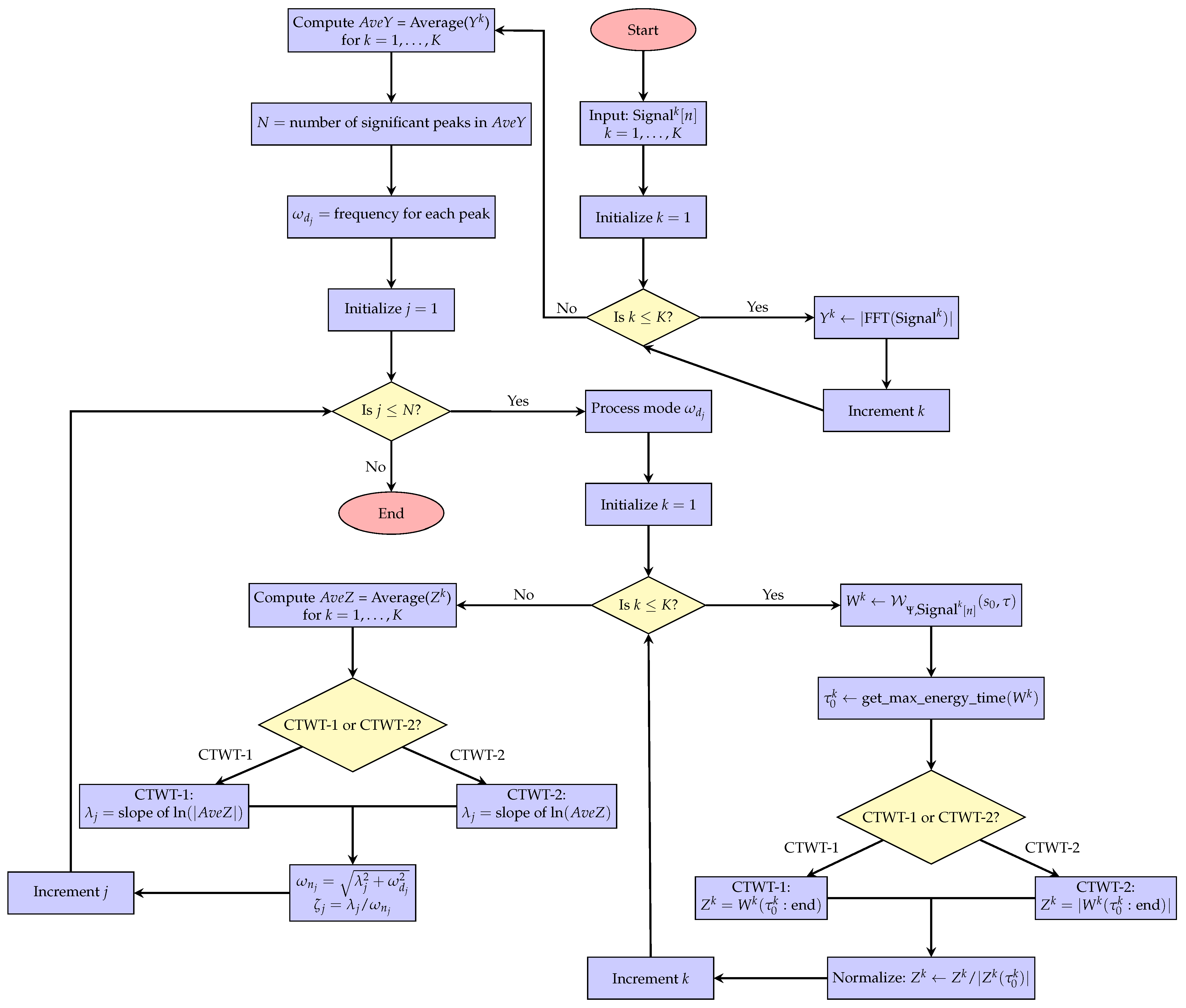
Algorithm 1: CTWT-1 and CTWT-2 Methods

Input: ${\mathrm{Signal}}^k\left[n\right]$ where $k=1,2,\cdots ,K$ represents the sample and K is the number of samples Output: ${\omega }_{n_j}$ and ${\zeta }_j$ for $j=1,2,\cdots ,N$ where N is the number of modes for $k=1,2,\cdots ,K$ do    $Y^k\leftarrow$ Compute the magnitude of $\mathrm{FFT}\left({\mathrm{Signal}}^k\left(n\right)\right)$ end for $AveY\leftarrow$ Average of $Y^k$ $N\leftarrow$ Number of significant peaks in $AveY$ ${\omega }_{d_j}\leftarrow$ Frequency corresponding to each significant peak in $AveY$ for each ${\omega }_{d_j}$ do    for $k=1,2,\cdots ,K$ do      $W^k\leftarrow$ Compute ${\mathcal{W}}_{\Psi ,{\mathrm{Signal}}^k\left[n\right]}(s_0,\tau )$ at scale $s_0$ corresponding to ${\omega }_{d_j}$ {Equation (21)}      ${\tau }_0^k\leftarrow$ get_max_energy_time($W^k$) {Maximum energy to estimate time of impact ((see Equation (4)))}      if CTWT-1 then         $Z^k\leftarrow W^k({\tau }_0^k:end)$ {Alignment in CTWT-1} else if CTWT-2 then         $Z^k\leftarrow \left|W^k({\tau }_0^k:end)\right|$ {Alignment in CTWT-2}      end if      $Z^k\leftarrow Z^k/\left|Z^k\left({\tau }_0^k\right)\right|$ {Normalizing to compensate the effect of $B^k$ (see Equation (4))}    end for    $AveZ\leftarrow$ Average of $Z^k$    if CTWT-1 then      ${\lambda }_j\leftarrow$ Slope of $ln\left(\right|AveZ\left|\right)$ {Equation (31)} else if CTWT-2 then      ${\lambda }_j\leftarrow$ Slope of $ln\left(AveZ\right)$    end if    ${\omega }_{n_j}\leftarrow \sqrt{{\lambda }_j^2+{\omega }_{d_j}^2}$ {Equation (3)}    ${\zeta }_j\leftarrow {\lambda }_j/{\omega }_{n_j}$ end for

1.

Estimation of Damping Frequencies: The initial phase of the algorithm focuses on the analysis of the FFT for each sample. By evaluating the FFT’s magnitude, represented by $Y^k$, we identify significant peaks. These peaks are indicative of the system’s modes, with the damping frequencies, ${\omega }_{d_j}$, corresponding to these peaks. Since individual samples might provide varying results, we average out the damping frequencies using the mean of all $Y^k$s.

2.

CTWT and Sample Alignment: Assuming that the system behaves similarly to an SDOF dynamic around each damped frequency, we determine the corresponding scale. At this designated scale, the CTWT is computed for every sample, denoted by $W^k$. A fundamental step in this phase involves the alignment of samples. Due to the variability in impact times across repeated measurements, we use the maximum energy point as an alignment reference. This reference point, which is an estimate of the time of impact, is obtained from the get_max_energy_time function. This function finds the maximum point after applying a Savitzky–Golay finite impulse response (FIR) smoothing filter to the input data. Data recorded prior to this point are disregarded. To account for the varying magnitudes of each impact, a normalization factor is incorporated before the averaging step.

3.

Averaging and Extraction of Damping Ratio: As the wavelet transform is linear, it retains the additive characteristics of Gaussian noise. The CTWT-1 approach involves averaging the complex-valued$Z^k$ values directly in the wavelet domain. This method aims to reduce noise while preserving the full complex signal information before further processing. Conversely, in the CTWT-2 approach, the averaging is performed after converting the complex values to real values by taking their absolute values. This distinction underscores the importance of the location where averaging occurs within the process, affecting the accuracy and reliability of the resulting damping ratio estimates. By employing Equations (3) and (31), the damping coefficient and damping ratio are obtained.

5. Results and Discussion

This section showcases the results of numerical simulations and experimental analyses conducted using Matlab. The aim is to assess the effectiveness of different algorithms in extracting the damping ratio. Our investigation incorporates established algorithms, including PP, pLSCF, LSRF, and Yoshida, alongside our proposed methods, CTWT-1 and CTWT-2. In our implementation, we utilize the built-in PP and LSRF algorithms in Matlab, as well as the algorithm described in [23] for the Yoshida method and the code provided by [40] for the pLSCF method.

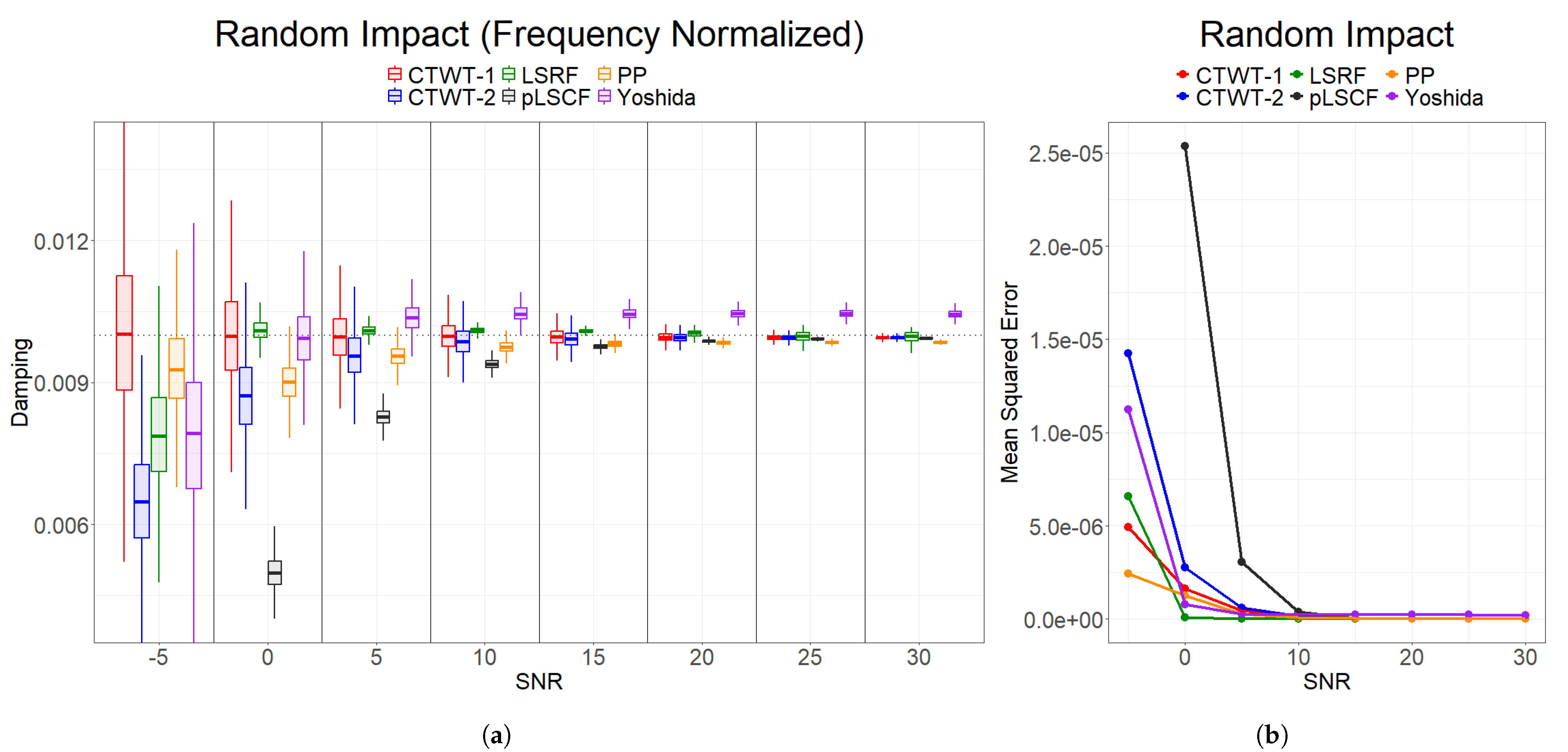
5.1. Numerical Simulation

The central signal guiding our investigation is ${\mathrm{Signal}}^k\left(t\right)=B^{k}x(t-{\tau }_0^k)+{ϵ}^k\left(t\right)$, which is articulated in Equation (4). This equation encapsulates various factors, such as amplitude variation $B_k$, time-shift ${\tau }_0^k$, and noise ${ϵ}_k\left(t\right)$, all of which affect the behavior of the signal. The influence of these parameters, together with the total number of recordings K, the correlation between the sampling frequency and the modal frequency, and the overall number of samples in each recording L, collectively shape the results of our algorithmic evaluations. To ensure a satisfactory resolution for capturing system dynamics, we selected a damping ratio of $\zeta =0.01$, a sampling frequency of $\mathrm{Fs}=800\mathrm{Hz}$, a signal length of $L=4000$, and damped frequency of ${\omega }_d=15.516\mathrm{Hz}$. To ensure reliability and conduct statistical analysis, each simulation was repeated 1000 times.

To determine the accuracy of damping ratio extraction by different algorithms, we used analysis of variance (ANOVA) testing in R with the null hypothesis that the number of samples has no effect on the output.

Table 1. The effect of the number of recordings in ANOVA test for aligned dataset.

Method	F	p-Value
CTWT-1	3.09	0.079
CTWT-2	5.91	0.015
LSRF	0.78	0.377
pLSCF	0.045	0.831
PP	0.625	0.429
Yoshida	0.47	0.493

summarizes the outcomes of this test for aligned recordings, in which the impact takes place at the start of the recordings (${\tau }_0^k=0$). The total number of recordings K varies from 10 to 100 with intervals of 10.

• The CTWT-2 method shows a significant effect of the number of samples on damping ratio estimates, with a relatively low p-value (0.015), indicating a notable influence of the number of recordings on its performance.
• The CTWT-1 method shows a moderate effect with a p-value of 0.079, suggesting some influence of the number of recordings, though less pronounced compared to CTWT-2.
• The LSRF method demonstrates a limited impact with a p-value of 0.377, suggesting lower sensitivity to the number of recordings compared to CTWT methods.
• The pLSCF method demonstrates a lower relative effect with a higher p-value of 0.831, indicating the least influence of the number of recordings on its performance.
• The PP and Yoshida methods also show limited effectiveness with p-values of 0.429 and 0.493, similar to the LSRF method.

These results suggest that, while the CTWT-2 method is significantly affected by the number of recordings, the CTWT-1 method shows a moderate effect, and the LSRF, pLSCF, PP, and Yoshida methods are less sensitive to variations in the number of samples.

In addition to examining the impact of the number of recordings, this article also explores the influence of noise on the performance of these damping ratio extraction methods. As illustrated in Figure 1, we evaluate how varying signal-to-noise ratios (SNRs) affect these methods. The analysis assumes that the time of impact is precisely known and occurs at the beginning of the recordings. The dashed line in the figure denotes the true value of the damping ratio. Our investigation contains a comprehensive range of SNR conditions, extending from −5 dB to 30 dB, thereby facilitating a thorough comparison of the efficacy of the different methodologies employed.

As depicted in this figure, all methods perform well at higher SNR levels. At an SNR of −5dB, the PP method shows the best performance, exhibiting the lowest error. Additionally, the CTWT-1 method performs commendably at this level of noise, surpassing the LSRF but not achieving the same level of performance as the PP method. At an SNR of 0dB, LSRF shows the best performance with the lowest error, indicating high accuracy and precision. When comparing the two CTWT methods, the CTWT-1 method consistently demonstrates strong performance across various SNR levels, resulting in lower errors. The box plots for CTWT-1 closely align with the true values. In contrast, CTWT-2 exhibits slightly higher error levels. This suggests that the differences in the averaging step between the two methods affect CTWT-2’s accuracy. Moreover, the Yoshida method performs similarly to the CTWT-2 method, with almost the same error levels. The mean squared error (MSE) for Yoshida is closely aligned with those for CTWT-2, indicating comparable accuracy. Furthermore, the pLSCF method begins to exhibit reduced performance at an SNR of 5dB, indicating a higher susceptibility to noise compared to other methods. While it is accurate at higher SNR levels, its performance deteriorates as the level of noise increases, falling behind other methods.

Figure 1 highlights the superior performance of the LSRF and PP methods, which stand out with the lowest error and highest precision across most SNR levels in scenarios where the impact is known to be at the beginning of the recorded signal. The CTWT-1 method follows closely, outperforming CTWT-2 and Yoshida. The Yoshida method, with almost the same accuracy as CTWT-2, demonstrates strong performance as well. The pLSCF method, though effective at higher SNR, becomes more sensitive to noise at lower SNR levels.

While Figure 1 demonstrates the damping ratio extraction methods assuming the impact is known to be at the beginning of the signal, this scenario is not realistic. In many practical situations, the exact time of impact is not fixed at the beginning. To address this, Figure 2 presents the scenario where the time of the impact is random but known. This more realistic condition reveals that variations in method performance are generally not significant, except for specific observations at higher SNR levels.

In this analysis, “frequency normalized” refers to the process in which we adjust for the frequency content of the impact. By knowing the time of impact, we can perform an FFT on the impact signal and then divide the FFT of the measurement signal by the FFT of the impact. This operation yields the system’s frequency response, which we can then use for damping extraction methods.

Comparing Figure 2 with Figure 1 suggests that the CTWT methods, LSRF, and pLSCF have maintained stable performance across varying conditions of impact timing, with minimal changes in error rates compared to the fixed impact scenario. This demonstrates robustness against timing variations, supporting their applicability in unpredictable environments. However, some differences were more pronounced under the random impact conditions at higher SNR levels. The PP method exhibited a slight worsening in performance, reflecting a decrease in effectiveness when faced with timing variations. The Yoshida method showed a significant decrease in performance at higher SNR levels, which emphasizes its vulnerability to timing variations. This decline suggests that, while the method can work well under ideal conditions, its reliability decreases significantly with more noise and timing variability.

Figure 1 and Figure 2 demonstrate the accuracy of the damping ratio extraction methods under the assumption that the exact impact time is known. However, this assumption may not be valid in practical applications, especially when no sensor is available on the hammer to detect the impact time. In FFT-based methods, normalization in the frequency domain requires an estimate of the impact time. Errors in this estimate can greatly reduce the accuracy of these methods.

Figure 3 shows how the accuracy of various damping ratio extraction methods degrades as the number of samples shifted from the actual impact time increases. The two subfigures display results for different SNR levels: Figure 3a 10 dB SNR and Figure 3b 0 dB SNR. As shown in this figure, even a small error in the impact time estimation can lead to significant variations in the damping ratio, with FFT-based methods showing high levels of sensitivity to these errors.

One approach to estimating the time of impact is through wavelet analysis, which identifies the point of maximum energy. This technique allows us to estimate the impact time even when the exact moment is unknown. By estimating the time of impact and computing the FFT of the impulse input, we can perform frequency normalization to assess the system’s frequency response. Figure 4 illustrates the outcomes achieved through wavelet analysis to determine the time of impact. Figure 4a displays the extracted distributions of the damping ratios for various methods across different SNR levels. Meanwhile, Figure 4b presents the MSE of the damping ratio estimates for the same methods. These figures emphasize the performance and reliability of the distributions under varying SNR conditions, demonstrating their effectiveness in scenarios where the precise time of impact is not clearly defined.

Analyzing the graphs, it is evident that different methods perform variably under non-aligned conditions. The damping ratio distribution in Figure 4a shows that methods like LSRF and CTWT-2 tend to have lower damping ratio variations, indicating higher accuracy. In contrast, the PP method shows higher variations, especially at lower SNR levels, suggesting lower robustness to noise. In terms of mean squared error, as shown in Figure 4b, the methods LSRF and CTWT-2 again demonstrate superior performance with lower MSE values across all SNR levels. This indicates the reliability and precision of these methods in generating accurate damping ratio estimates under non-aligned conditions. The pLSCF method also performs well at higher SNR levels but displays higher sensitivity to increased noise levels, leading to a dramatic decrease in performance as the SNR decreases. The PP method exhibits the highest MSE values even in lower levels of noise, indicating it is less effective in estimating damping ratios when the impact time is not precisely known. The CTWT-1 method performs comparably to LSRF, CTWT-2, and pLSCF at high SNR levels, demonstrating its reliability under less noisy conditions. However, as the SNR decreases, CTWT-1 shows more robustness compared to pLSCF but is less effective compared to LSRF and CTWT-2. The Yoshida method performs better than CTWT-1 at low SNR levels but is worse than CTWT-2 and LSRF. Additionally, it has higher MSE values at high SNR levels compared to other methods. In conclusion, the LSRF and CTWT-2 methods emerge as the most robust and accurate for damping ratio estimation under non-aligned conditions, due to their lower variation in damping ratios and lower mean squared error values across different SNR levels. These findings demonstrate the importance of choosing reliable methods for practical applications where the exact impact time is uncertain.

While examining the performance of damping ratio extraction methods under various SNR conditions provides valuable insights, it is also crucial to understand the impact of the number of recordings on these estimates. In practical applications, the number of recordings can vary, affecting the reliability and accuracy of the methods. To investigate this, we conducted an ANOVA test to analyze the effect of the number of recordings on damping ratio estimates using a non-aligned dataset. The results are presented in

Table 2. ANOVA test results showing the effect of the number of recordings on damping ratio estimates using non-aligned dataset.

Method	F	p-Value
CTWT-1	2.49	0.114
CTWT-2	1.52	0.217
LSRF	1.16	0.282
pLSCF	64.0	1.27 × 10−15
PP	889.0	2.21 × 10−194
Yoshida	0.002	0.969

.

From the table, we observe the following:

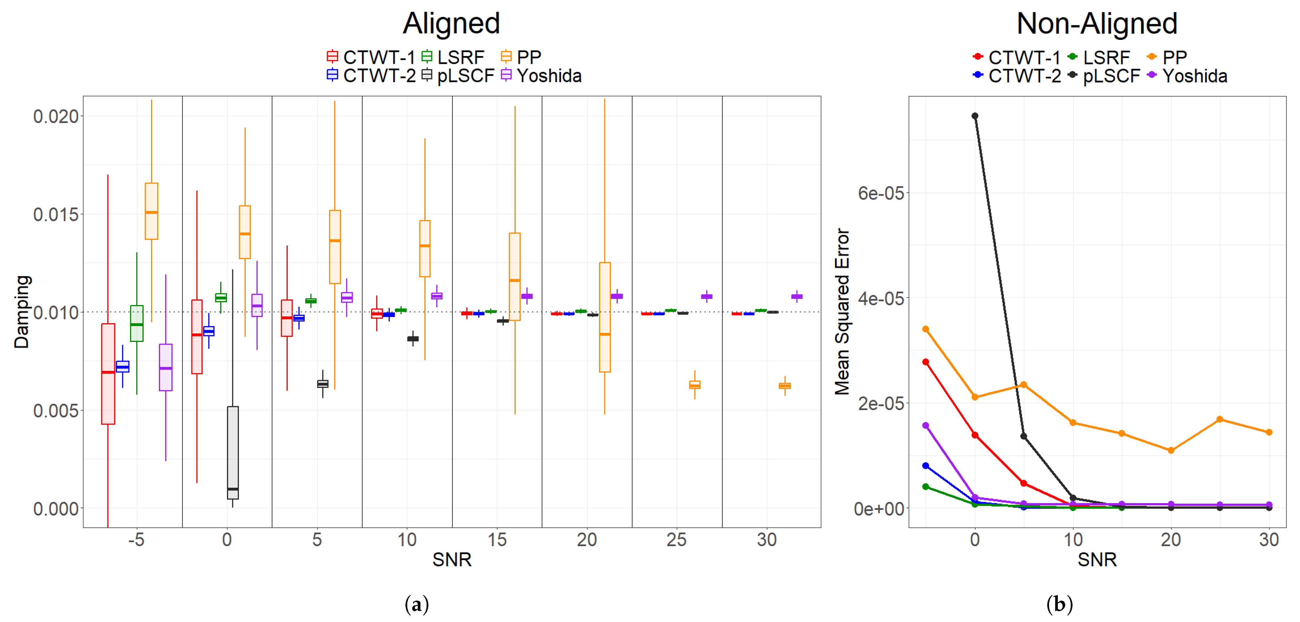
• The PP method shows a highly significant effect of the number of samples on damping ratio estimates, with an extremely low p-value ($2.21\times {10}^{-194}$), indicating a strong influence of the number of recordings on its performance.
• The pLSCF method also shows a significant effect with a p-value of $1.27\times {10}^{-15}$, although the influence is less pronounced compared to the PP method.
• The CTWT-1, CTWT-2, LSRF, and Yoshida methods do not show significant effects of the number of samples on damping ratio estimates, as indicated by their high p-values.

These results suggest that, while the PP and pLSCF methods are significantly affected by the number of recordings, the CTWT-1, CTWT-2, LSRF, and Yoshida methods are less influenced by the number of samples. This robustness further underscores the suitability of the LSRF and CTWT-2 methods for practical applications where the number of recordings may vary, alongside their previously noted accuracy and reliability under non-aligned conditions. In summary, the LSRF and CTWT-2 methods are not only accurate and reliable under varying SNR levels but also robust to the effect of the number of recordings, making them highly suitable for real-world applications where both impact time and the number of recordings are uncertain. The ANOVA test results for both the aligned (Table 1) and non-aligned (Table 2) datasets reveal key differences in the sensitivity of damping ratio estimation methods to the number of recordings. For the CTWT-1 method, a moderate effect is observed in the aligned dataset with a p-value of 0.079, indicating some sensitivity to the number of recordings, while this effect diminishes in the non-aligned dataset with a p-value of 0.114, suggesting reduced sensitivity when the impact time is variable. The CTWT-2 method shows a significant effect in the aligned dataset with a p-value of 0.015, indicating notable sensitivity to the number of recordings, but this effect lessens in the non-aligned dataset with a p-value of 0.217. The LSRF method exhibits minimal sensitivity to the number of recordings in both scenarios, with p-values of 0.377 and 0.282 for aligned and non-aligned datasets, respectively. In contrast, the pLSCF method displays negligible sensitivity in the aligned dataset with a high p-value of 0.831, but becomes highly sensitive in the non-aligned scenario, with a very low p-value of $1.27\times {10}^{-15}$. Similarly, the PP method, which shows limited effect in the aligned dataset (p-value of 0.429), exhibits extreme sensitivity to the number of recordings in non-aligned conditions, as evidenced by a p-value of $2.21\times {10}^{-194}$. The Yoshida method maintains robustness across both conditions, with high p-values of 0.493 and 0.969 in the aligned and non-aligned datasets, respectively, indicating low sensitivity to the number of recordings.

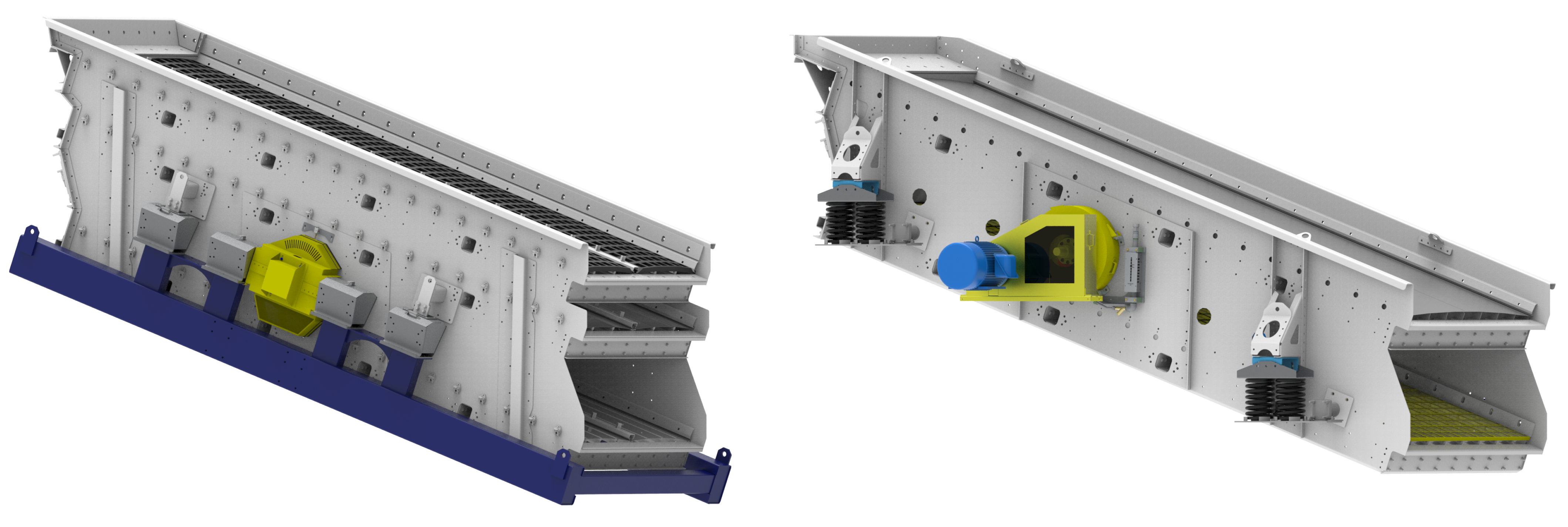
5.2. Experimental Analysis

The research presented here was motivated by the need to conduct modal analysis on vibrating screens. Vibrating screens, depicted in Figure 5, are large machines used to separate materials by size using screens that are stimulated with an unbalanced rotating shaft. These machines are unique in vibration analysis as they are designed to vibrate at specific frequencies rather than suppress vibrations completely. The machines we examine weigh several metric tons, have different drive geometries, and are suspended on springs and/or dampers. Typically, these machines operate in the 10–20 Hz range, with free body modes in the 1–5 Hz range.

We conducted hammer impact tests using four and eight accelerometers connected wirelessly to collect the data. We used a real dataset containing 40 recordings to further validate our findings. For statistical analyses, they were separated into 10 groups of four. The extracted damping ratios and the variances for each method are summarized in

Table 3. Results of damping ratio estimates and variances for different methods across frequencies.

Method	4.71 Hz		17.81 Hz		27.68 Hz
	Damping Ratio	Variance	Damping Ratio	Variance	Damping Ratio	Variance
CTWT-1	0.0308	2.72 × 10−4	0.0086	1.52 × 10−6	0.0093	2.14 × 10−6
CTWT-2	0.0482	1.58 × 10−6	0.0084	2.11 × 10−9	0.0092	1.20 × 10−9
LSRF	0.0411	2.09 × 10−4	0.0090	2.32 × 10−5	0.0088	7.85 × 10−7
pLSCF	0.0210	1.17 × 10−4	0.0034	1.02 × 10−7	0.0032	5.48 × 10−6
PP	0.0521	1.09 × 10−3	0.0074	4.98 × 10−6	0.0094	4.13 × 10−6
Yoshida	0.0150	2.03 × 10−4	0.0058	7.03 × 10−6	0.0040	2.17 × 10−5

.

The results in this table illustrate the variability in damping ratio estimates and variances across different methods and frequencies. Although the true damping ratio is unknown, simulations suggested that the LSRF and CTWT-2 methods would perform well; however, the real data indicate some discrepancies from those expectations.

At 4.71 Hz, the CTWT-2 method provides a damping ratio of 0.0482 with a variance of $1.58\times {10}^{-6}$, indicating strong stability and reliability. The PP method gives a damping ratio close to that of CTWT-2 at 0.0521 but has the highest variance ($1.09\times {10}^{-3}$), indicating greater uncertainty. Similarly, the LSRF method also provides a damping ratio close to CTWT-2 at 0.0411 but with a higher variance ($2.09\times {10}^{-4}$). This suggests that, while these methods yield similar damping ratio estimates, CTWT-2 offers more consistent results at this frequency. Conversely, CTWT-1, pLSCF, and Yoshida show damping ratios much lower than CTWT-2 and LSRF, which performed best in simulations.

For 17.81 Hz, the CTWT-2 method again stands out with the lowest variance ($2.11\times {10}^{-9}$), suggesting high stability in its estimates. The LSRF method provides a damping ratio close to CTWT-2 at 0.0090, but with the highest variance ($2.32\times {10}^{-5}$), indicating potential instability. CTWT-1 also offers a damping ratio estimate close to CTWT-2, reinforcing its reliability. The PP method similarly provides a close estimate, showing consistent performance. In contrast, the Yoshida method’s estimate diverges more from the CTWT-2 and LSRF estimates, while the pLSCF method exhibits a greater difference.

At 27.68 Hz, CTWT-2 continues to provide the lowest variance ($1.20\times {10}^{-9}$), reinforcing its reliability. The CTWT-1 method also gives damping ratios close to CTWT-2 at this frequency, demonstrating consistent performance. The PP method performs well, offering estimates close to CTWT-2. However, the pLSCF and Yoshida methods produce estimates that are significantly different from the rest, indicating less alignment with the more reliable methods.

Also, the identified damping ratios exhibit greater consistency at higher frequencies. At lower frequencies, even minor inaccuracies in frequency determination can lead to substantial relative errors, thereby significantly affecting the accuracy of the damping ratio estimates. Conversely, at higher frequencies, the influence of frequency errors is diminished, resulting in more stable and reliable outcomes.

Overall, while simulations suggested that LSRF and CTWT-2 would be among the best performers, the actual data indicate that CTWT-2 consistently delivers the lowest variances across all frequencies, marking it as a reliable method for damping ratio estimation. CTWT-1 provides damping ratios close to CTWT-2 at higher frequencies but with higher variances, indicating less stability. The PP method performs well across frequencies, offering estimates close to CTWT-2. The Yoshida and pLSCF methods have different damping values compared to the CTWT, LSRF, and PP methods and may exhibit higher errors. Based on simulation results, the CTWT-2 method is likely closer to the true value. Despite its inconsistency, the pLSCF method’s speed may offer advantages in scenarios where quick estimation is necessary, despite its challenges in producing consistent results.

6. Conclusions

The findings presented in this article emphasize the critical need for robust modal analysis methods that can effectively address the complexities and unpredictability inherent in real-world applications. A key challenge frequently encountered in these settings is the misalignment of signals—a common issue that traditional modal analysis approaches often fail to adequately address due to their reliance on idealized conditions. To address this challenge, we leveraged wavelet energy for improved alignment and averaging, ensuring a more robust and reliable damping estimation process. This approach enhances the ability to extract meaningful damping characteristics even in the presence of non-synchronized recordings. The demonstrated resilience of our proposed methods makes them highly suitable for a broad range of applications, from structural health monitoring in civil engineering to diagnostic techniques in machinery maintenance, where achieving precise damping extraction is vital.

However, despite these advantages, this study has certain limitations that should be acknowledged. One key limitation is the presence of nonlinear effects in real-world applications, which may introduce additional complexities that were not explicitly modeled in this study. Additionally, closely spaced modes can be difficult to distinguish, particularly in highly damped systems where frequency separation is minimal. Another challenge is that our method assumes an ideal impact event for estimating the maximum energy, whereas in large industrial machines, impact conditions can be highly variable and less controlled. Furthermore, wavelet analysis is affected by edge effects, necessitating sufficiently long recordings to maintain accuracy. This means that the proposed method may not perform as well when working with short-duration recordings, limiting its applicability in certain real-world scenarios. To further enhance the robustness and applicability of the proposed methods, future research should explore several key improvements. One promising direction is the exploration of alternative wavelet types, particularly those with non-Gaussian windows, to mitigate edge effects while still providing sufficient mode separation. Additionally, refining the method to improve its performance in the presence of nonlinear damping behaviors extends its real-world applicability. Finally, validating the approach on a broader range of industrial and large-scale structures would provide deeper insights into its practical effectiveness.

Overall, this study establishes a strong foundation for advancing wavelet-based damping extraction, demonstrating its potential while also highlighting the need for continued refinements to optimize its performance in complex real-world conditions.

References

1. Ewins, D.J. Modal Testing: Theory, Practice and Application; John Wiley & Sons: Hoboken, NJ, USA, 2009. [Google Scholar]
2. Chopra, A.K. Dynamics of Structures; Pearson Education India: Tamil Nadu, India, 2007. [Google Scholar]
3. Inman, D.J.; Singh, R.C. Engineering Vibration; Prentice Hall Englewood Cliffs: Englewood Cliffs, NJ, USA, 1994; Volume 3. [Google Scholar]
4. Rao, S.S.; Yap, F.F. Mechanical Vibrations; Addison-Wesley: New York, NY, USA, 1995. [Google Scholar]
5. Barattini, C.; Dimauro, L.; Vella, A.D.; Vigliani, A. Dynamic Analysis of a High-Performance Prosthetic Leg: Experimental Characterisation and Numerical Modelling. Appl. Sci. 2023, 13, 11566. [Google Scholar] [CrossRef]
6. Liu, D.; Tang, Z.; Bao, Y.; Li, H. Machine-learning-based methods for output-only structural modal identification. Struct. Control. Health Monit. 2021, 28, e2843. [Google Scholar] [CrossRef]
7. Santos, J.; Crémona, C.; Silveira, P. Automatic operational modal analysis of complex civil infrastructures. Struct. Eng. Int. 2020, 30, 365–380. [Google Scholar] [CrossRef]
8. Wang, C.; Huang, H.; Lai, X.; Chen, J. A New Online Operational Modal Analysis Method for Vibration Control for Linear Time-Varying Structure. Appl. Sci. 2020, 10, 48. [Google Scholar] [CrossRef]
9. Soria, L.; Peeters, B.; Anthonis, J. Operational modal analysis and the performance assessment of vehicle suspension systems. Shock Vib. 2012, 19, 1099–1113. [Google Scholar] [CrossRef]
10. Feng, Z.; Liang, M.; Chu, F. Recent advances in time–frequency analysis methods for machinery fault diagnosis: A review with application examples. Mech. Syst. Signal Process. 2013, 38, 165–205. [Google Scholar] [CrossRef]
11. Zhang, Y.; Randall, R. Rolling element bearing fault diagnosis based on the combination of genetic algorithms and fast kurtogram. Mech. Syst. Signal Process. 2009, 23, 1509–1517. [Google Scholar] [CrossRef]
12. He, J.; Fu, Z.F. 1—Overview of modal analysis. In Modal Analysis; He, J., Fu, Z.F., Eds.; Butterworth-Heinemann: Oxford, UK, 2001; pp. 1–11. [Google Scholar] [CrossRef]
13. Slavič, J.; Simonovski, I.; Boltežar, M. Damping identification using a continuous wavelet transform: Application to real data. J. Sound Vib. 2003, 262, 291–307. [Google Scholar] [CrossRef]
14. Staszewski, W. Identification of damping in MDOF systems using time-scale decomposition. J. Sound Vib. 1997, 203, 283–305. [Google Scholar] [CrossRef]
15. Brincker, R.; Zhang, L.; Andersen, P. Modal identification of output-only systems using frequency domain decomposition. Smart Mater. Struct. 2001, 10, 441. [Google Scholar] [CrossRef]
16. Wang, Y.; Egner, F.S.; Willems, T.; Kirchner, M.; Desmet, W. Camera-based experimental modal analysis with impact excitation: Reaching high frequencies thanks to one accelerometer and random sampling in time. Mech. Syst. Signal Process. 2022, 170, 108879. [Google Scholar] [CrossRef]
17. Nadkarni, I.; Bhardwaj, R.; Ninan, S.; Chippa, S. Experimental modal parameter identification and validation of cantilever beam. Mater. Today Proc. 2021, 38, 319–324. [Google Scholar] [CrossRef]
18. Li, M.; Lu, Z.; Cao, Q.; Gao, J.; Hu, B. Automatic assessment method and device for depression symptom severity based on emotional facial expression and pupil-wave. IEEE Trans. Instrum. Meas. 2024, 73, 1–15. [Google Scholar] [CrossRef]
19. Zhang, S.; Qu, N.; Zheng, T.; Hu, C. Series arc fault detection based on wavelet compression reconstruction data enhancement and deep residual network. IEEE Trans. Instrum. Meas. 2022, 71, 1–9. [Google Scholar] [CrossRef]
20. Albaqami, H.; Hassan, G.M.; Subasi, A.; Datta, A. Automatic detection of abnormal EEG signals using wavelet feature extraction and gradient boosting decision tree. Biomed. Signal Process. Control. 2021, 70, 102957. [Google Scholar] [CrossRef]
21. Boltežar, M.; Slavič, J. Enhancements to the continuous wavelet transform for damping identifications on short signals. Mech. Syst. Signal Process. 2004, 18, 1065–1076. [Google Scholar] [CrossRef]
22. Tomac, I.; Slavič, J. Damping identification based on a high-speed camera. Mech. Syst. Signal Process. 2022, 166, 108485. [Google Scholar] [CrossRef]
23. Zieliński, T.P.; Duda, K. Frequency and damping estimation methods-an overview. Metrol. Meas. Syst. 2011, 18, 505–528. [Google Scholar] [CrossRef]
24. Slavič, J.; Boltežar, M. Damping identification with the Morlet-wave. Mech. Syst. Signal Process. 2011, 25, 1632–1645. [Google Scholar] [CrossRef]
25. Tomac, I.; Lozina, Ž.; Sedlar, D. Extended Morlet-Wave damping identification method. Int. J. Mech. Sci. 2017, 127, 31–40. [Google Scholar] [CrossRef]
26. Zrayka, A.K.; Mucchi, E. A comparison among modal parameter extraction methods. SN Appl. Sci. 2019, 1, 781. [Google Scholar] [CrossRef]
27. Tomac, I.; Slavič, J. Morlet-wave-based modal identification in the time domain. Mech. Syst. Signal Process. 2023, 192, 110243. [Google Scholar] [CrossRef]
28. Xu, H.; Liu, Y.; Chen, J.; Yang, D.; Yang, Y. Novel formula for determining bridge damping ratio from two wheels of a scanning vehicle by wavelet transform. Mech. Syst. Signal Process. 2024, 208, 111026. [Google Scholar] [CrossRef]
29. Janeliukstis, R. Continuous wavelet transform-based method for enhancing estimation of wind turbine blade natural frequencies and damping for machine learning purposes. Measurement 2021, 172, 108897. [Google Scholar] [CrossRef]
30. Wang, S.; Zhao, W.; Zhang, G.; Xu, H.; Du, Y. Identification of structural parameters from free vibration data using Gabor wavelet transform. Mech. Syst. Signal Process. 2021, 147, 107122. [Google Scholar] [CrossRef]
31. Silva-Navarro, G.; Beltran-Carbajal, F.; Trujillo-Franco, L.G.; Peza-Solis, J.F.; Garcia-Perez, O.A. Online estimation techniques for natural and excitation frequencies on MDOF vibrating mechanical systems. Actuators 2021, 10, 41. [Google Scholar] [CrossRef]
32. Meirovitch, L. Fundamentals of Vibrations; Waveland Press: Long Grove, IL, USA, 2010. [Google Scholar]
33. Liu, M.; Gorman, D.G. Formulation of Rayleigh damping and its extensions. Comput. Struct. 1995, 57, 277–285. [Google Scholar] [CrossRef]
34. A Hasan, M.D.; Ahmad, Z.; Salman Leong, M.; Hee, L. Enhanced frequency domain decomposition algorithm: A review of a recent development for unbiased damping ratio estimates. J. Vibroeng. 2018, 20, 1919–1936. [Google Scholar] [CrossRef]
35. Døssing, O. Structural testing. Brüel Kjær (Ed.) 1988, 2, 1–54. [Google Scholar]
36. Sanchez, H.; Nova, F.; González-Estrada, O. Implementation of the Operational Modal Analysis technique in a power transmission shaft. Phys. Conf. Ser. 2019, 1247, 012032. [Google Scholar] [CrossRef]
37. Ozdemir, A.A.; Gumussoy, S. Transfer function estimation in system identification toolbox via vector fitting. IFAC-PapersOnLine 2017, 50, 6232–6237. [Google Scholar] [CrossRef]
38. Sanathanan, C.; Koerner, J. Transfer function synthesis as a ratio of two complex polynomials. IEEE Trans. Autom. Control. 1963, 8, 56–58. [Google Scholar] [CrossRef]
39. El-kafafy, M.; De Troyer, T.; Peeters, B.; Guillaume, P. Fast maximum-likelihood identification of modal parameters with uncertainty intervals: A modal model-based formulation. Mech. Syst. Signal Process. 2013, 37, 422–439. [Google Scholar] [CrossRef]
40. Trumpp, R.F. Implementierung des Poly-reference Least Square Complex Frequency (p-LSCF) Algorithmus zur Operational Modal Analysis (OMA). Bachelor’s Thesis, Karlsruhe Institute of Technology (KIT), Karlsruhe, Germany, 2017. [Google Scholar]
41. Guillaume, P.; Verboven, P.; Vanlanduit, S.; Van Der Auweraer, H.; Peeters, B. A poly-reference implementation of the least-squares complex frequency-domain estimator. In Proceedings of the IMAC; A Conference & Exposition on Structural Dynamics, Society for Experimental, Kissimmee, FL, USA, 3–6 February 2003; Volume 21. [Google Scholar]
42. Junsheng, C.; Dejie, Y.; Yu, Y. Time–energy density analysis based on wavelet transform. Ndt E Int. 2005, 38, 569–572. [Google Scholar] [CrossRef]
43. Chen, S.L.; Liu, J.J.; Lai, H.C. Wavelet analysis for identification of damping ratios and natural frequencies. J. Sound Vib. 2009, 323, 130–147. [Google Scholar] [CrossRef]
Figure 1. Comparison of damping ratio extraction methods across varying SNR levels when the impact is known to be at the beginning of the signal. The dashed line represents the true damping ratio value. (a) Shows the damping ratio performance, while (b) presents the mean squared error performance. LSRF consistently exhibits the lowest error, demonstrating superior performance. (a) Damping Ratio vs. SNR. (b) Mean Squared Error vs. SNR.
Signals 06 00013 g001
Figure 2. Analysis of damping ratio extraction methods with random but known times of impact, frequency normalized. The figures show how each method performs when the impact timing is not fixed, presenting a more challenging but realistic scenario. (a) Damping Ratio vs. SNR. (b) Mean Squared Error vs. SNR.
Signals 06 00013 g002
Figure 3. Impact of sample shift on the accuracy of damping ratio extraction methods at 10dB SNR (a) and 0dB SNR (b), illustrating the degradation in performance with increasing misalignment from the true impact time. (a) 10 SNR. (b) 0 SNR.
Signals 06 00013 g003
Figure 4. (a,b) Damping ratio distribution and mean squared error of damping ratio estimates, respectively, for various methods using wavelet analysis to determine the time of impact across different signal-to-noise ratio (SNR) levels. These figures highlight the robustness and reliability of the methods under non-aligned conditions, when the time of impact is unknown. (a) Damping Ratio vs. SNR. (b) Mean Squared Error vs. SNR.
Signals 06 00013 g004
Figure 5. Vibrating screens.
Signals 06 00013 g005