Vision-Based Object Localization and Classification for Electric Vehicle Driving Assistance

Abstract

The continuous advances in intelligent systems and cutting-edge technology have greatly influenced the development of intelligent vehicles. Recently, integrating multiple sensors in cars has improved and spread the advanced drive-assistance systems (ADAS) solutions for achieving the goal of total autonomy. Despite current self-driving approaches and systems, autonomous driving is still an open research issue that must guarantee the safety and reliability of drivers. This work employs images from two cameras and Global Positioning System (GPS) data to propose a 3D vision-based object localization and classification method for assisting a car during driving. The experimental platform is a prototype of a two-sitter electric vehicle designed and assembled for navigating the campus under controlled mobility conditions. Simultaneously, color and depth images from the primary camera are combined to extract 2D features, which are reprojected into 3D space. Road detection and depth features isolate point clouds representing the objects to construct the occupancy map of the environment. A convolutional neural network was trained to classify typical urban objects in the color images. Experimental tests validate car and object pose in the occupancy map for different scenarios, reinforcing the car position visually estimated with GPS measurements.

1. Introduction

In recent years, the autonomous vehicle (AV) has been a broad field of academic and industrial research around topics like safety, electro-mobility, and autonomous driving. The increase in computing power has launched the integration of multi-sensors towards ADAS in vehicles for achieving autonomy. Simultaneously, machine learning algorithms implement system intelligence in ADAS to provide valuable and current information from the environment. However, a vehicle’s primary goal is not limited to transportation, but includes comfort, safety, and convenience.

Technological advancements have transformed the traditional automotive industry from old-fashioned travel sources into fully functional and intelligent machines that make travel easier [1]. Autonomous vehicles support functions like sensing the environment, connecting to the internet, obeying traffic guidelines, self-driving, and making quick decisions. Some motivations behind the research and development of AV is increasing driving safety and expanding the infrastructure of multi-services delivering [2].

Research laboratories, universities, and companies worldwide have developed autonomous and driverless cars. The Society of Automotive Engineers (SAE) [3] has published a classification based on the human intervention required to drive for measuring the autonomy of self-driving cars. Autonomy levels range from Level 0, where the car system briefly assists the driver, to Level 5, where human intervention is unnecessary [4]. The architecture of self-driving cars carries out two tasks: perception and decision. The perception task performs localization, road mapping, moving obstacle tracking, and traffic signal recognition. The decision task involves path planning, behavior selection, obstacle avoidance, and control. Moreover, the perception task estimates the state of the car and creates an internal representation of the environment using raw sensor data.

Among the typical sensors used in AVs is Light Detection and Ranging (LiDAR), Radio Detection and Ranging (RADAR), depth and color cameras, GPS, Inertial Measurement Unit (IMU), and odometers. Hence, various localization methods have alternatively been proposed: LiDAR-based, LiDAR plus camera-based, and camera-based [5]. A recent trend combines multisensor data to scan reliable and diverse measurements. For instance, LiDAR and visual data are simultaneously used for classification [6]. Likewise, in [7], a system uses LiDAR data and images to detect three-dimensional space. After noise removal, the Random Sample Consensus (RANSAC) method segments the ground and objects. Interpolation allows for accurate object data definition. Image objects with 3D points pose are matched; finally, the You Only Look Once (YOLO) [8] performs object recognition.

In [9], the vehicle localization task is based on sensor fusion, including an odometer, a GPS, and a visual sensor. However, some real constraints must be considered, such as GPS signal reception in areas impeded by trees, tunnels, and roads surrounded by large buildings. Cameras integrated into vehicles are becoming standard for their safety, low cost, and easy installation, providing more information than other conventional sensors [10]. Typically, motion control of an AV is achieved by analyzing the images acquired by onboard cameras and using neural networks [11]. Semantic segmentation and object detection based on Convolutional Neural Networks (CNNs) provide valuable data for making decisions in path planning [12].

In [13], the authors divide en grayscale channels to improve the visual objects; the next step is to implement a morphology method preprocessing image to produce a better binary image.

In [14], the authors used deeper CNN models and trained a sub-scale radio-controlled car to navigate off-road in the DARPA Autonomous Vehicle project. The model was trained with images acquired from two forward-facing cameras. Using a six-layer CNN, the model learned to navigate around obstacles while driving at a speed of 2 m/s. Moreover, in [15], the authors used supervised learning to steer an AV for making an end-to-end lateral vehicle controller using a CNN. The training data were the steering angle and the images acquired by the front-facing camera as a human-driven vehicle was used in a CarSim simulation [16]. The end-to-end learning-based method was recently proposed to infer the vehicles’ control value directly from the dashboard camera [12]. The approach presented in [17] considers the temporal structure of a dashboard camera to learn a generic driving model.

As these techniques use neural networks, correct parameter handling must be considered if their efficiency is to be improved. There are some quantization techniques to reduce memory footprint and latency [18], as well as methods to reduce the influence of parameter selection such as the via class-aware trace ratio optimization (CATRO) method [19] or the Sparce Connectivity Learning (SCL) method [20], which can be applied to different network architectures. More specifically, for object classification, the SqueezeNet model could serve as a practical choice for minimizing memory size, especially when the primary focus is on reducing the processing time [21].

Exploring lightweight AI models represents a promising solution for enhancing object classification methodology with a low memory size, demonstrating positive outcomes in their practical application [22]. Mobile-NetV2 is another option of CNN to implement in mobile devices, reducing memory use on real-time applications [23].

Multi-sensor data are used for simultaneous localization and mapping (SLAM), representing the fundamental tasks to solve in autonomous vehicles. SLAM consists of constructing a map of an unknown environment while simultaneously inferring the vehicle’s pose within the map [24]. The primary sensors employed for SLAM are LiDAR and cameras. In addition, visual SLAM (vSLAM) methodologies have become the mainstream for initializing the features and mapping for autonomous vehicle applications [25]. vSLAM is divided into two categories: direct SLAM and feature-based SLAM, which is the first track of a new frame by directly optimizing over pixel intensities. Meanwhile, feature-based SLAM infers the pose of a new frame by extracting sparse features, matching them to the features in a local map, and optimizing reprojection errors. In [26], a vSLAM-based localization system for indoors creates the environment map and localizes the camera pose in the maps. In [24], an improved multi-sensor fusion positioning system based on GNSS, LiDAR, cameras, and IMU with graph optimization is presented to improve the accuracy of vehicle pose. Similarly, the authors of [27] propose a novel visual-inertial simultaneous localization and mapping (VI-SLAM) method for intelligent navigation systems to overcome the posed challenges of car dynamics or large-scale outdoor environments.

On the other hand, the rapid development of the automotive sector requires dramatically reducing fossil fuel consumption. As most gasoline-powered vehicles produce gas emissions, the electric vehicle provides an alternative [28]. Implementing an exclusive lane for AVs employs connected multi-sensors to incorporate the vehicle when it is out of the controlled lane. 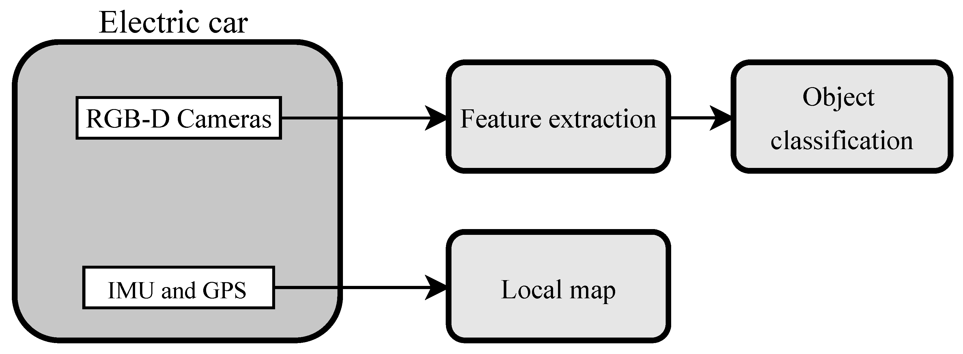This approach has been demonstrated to reduce the traffic flow along the way, improving travel time in autonomous connected systems [29]. Moreover, current vehicles are equipped with autonomous parking, visual object featuring and estimation, global positioning in real-time, and additional features for achieving the maximal level of autonomous driving. Although reliable results have already been proposed in this context, great challenges of performance and rapid response to critical events remain. Visual-based approaches have provided reliable solutions to real-time problems such as visual odometry, object detection, and classification. Therefore, this work analyses visual and pose data using vSLAM and ORB to detect and localize objects for constructing an occupancy map of a controlled urban environment. This map assists the navigation of an electric car, as illustrated in Figure 1. The car prototype navigates around the university campus in an outdoor urban context, representing a velocity-controlled scene with different obstacles such as safety cones, cars, trees, and traffic signs. The controlled conditions facilitate the use of fewer sensors mounted in the vehicle, including two color-depth cameras, IMU, and GPS sensors. The contributions of this work are as follows: (1) construct a sparse scene representation based on point clouds and than map to a 2D occupancy map for visualizing the occupied cells and reducing the stored and processed data; (2) provide a dataset of visual information, global pose, and inertial coordinates acquired from sensors mounted on the electric car; (3) five navigation environments have been arranged differently to validate the occupancy map constructed with the initial map and to classify the objects in the path. This work represents the first stage for achieving an autonomous electric vehicle.

The rest of the paper is organized as follows: Section 2 describes the experimental platform, data sensors, and proposed methodology. Next, Section 3 analyses the occupancy map, object location, and the classification obtained with our approach. Then, Section 4 presents a discussion of the different scenarios evaluated. Finally, Section 5 shows the conclusions.

2. Materials and Methods

2.1. Overall Navigation Strategy

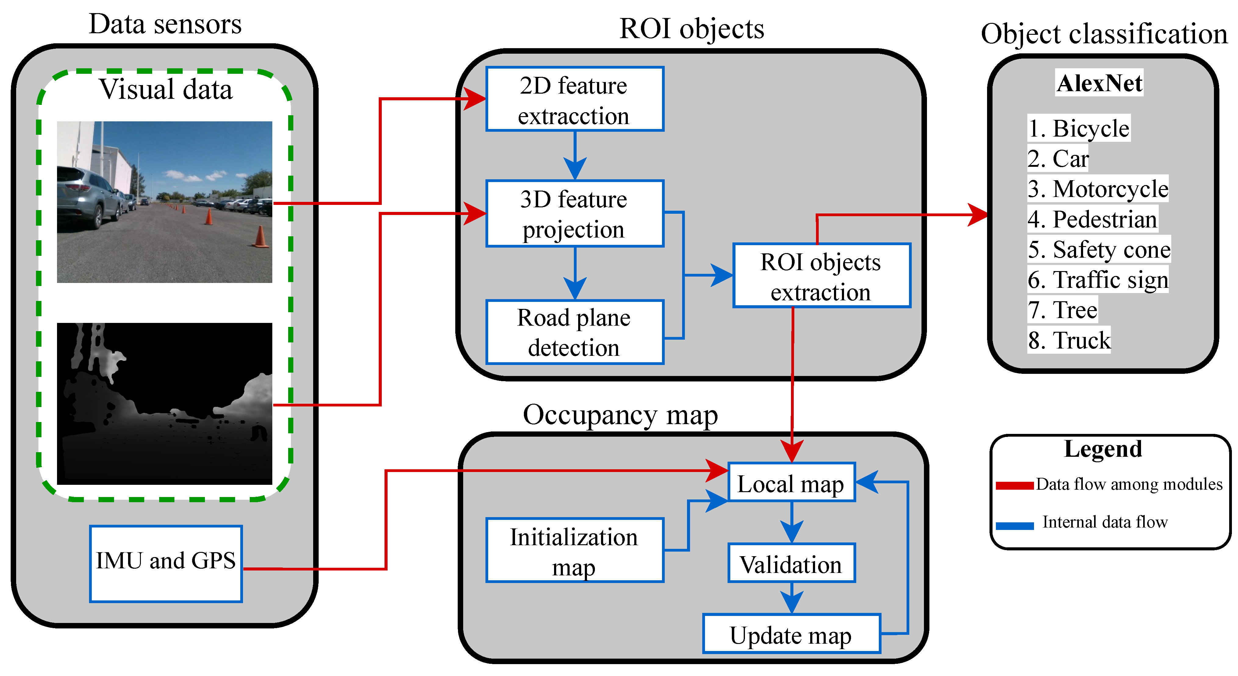
Figure 2 details the proposed vision-based object localization and classification method. Image, IMU, and GPS data were synchronously acquired during vehicle navigation around the campus limits. IMU and GPS provided positioning data, while the images captured what was in front of the vehicle. Images were captured at a rate of 21 fps, and IMU and GPS data were acquired at five samples per second. The color image’s most representative 2D feature points were extracted and projected to a 3D plot employing the depth image. The local road plane was calculated to separate only the point clouds belonging to the objects, facilitating the delimitation of objects’ regions of interest in the color image. The object’s regions were mapped from 3D to 2D coordinates in an occupancy map to validate the local object position with the initial occupancy map and to update the global occupancy map. Simultaneously, the extracted object’s regions in the color images were classified using a convolutional network based on AlexNet architecture. The electric car prototype navigated and concurrently detected, localized, and classified objects in the path; GPS monitored the vehicle pose for validating a straight trajectory. The point clouds and the 2D local map for visualizing the occupied cells reduced the stored and processed data during the vehicle navigation.

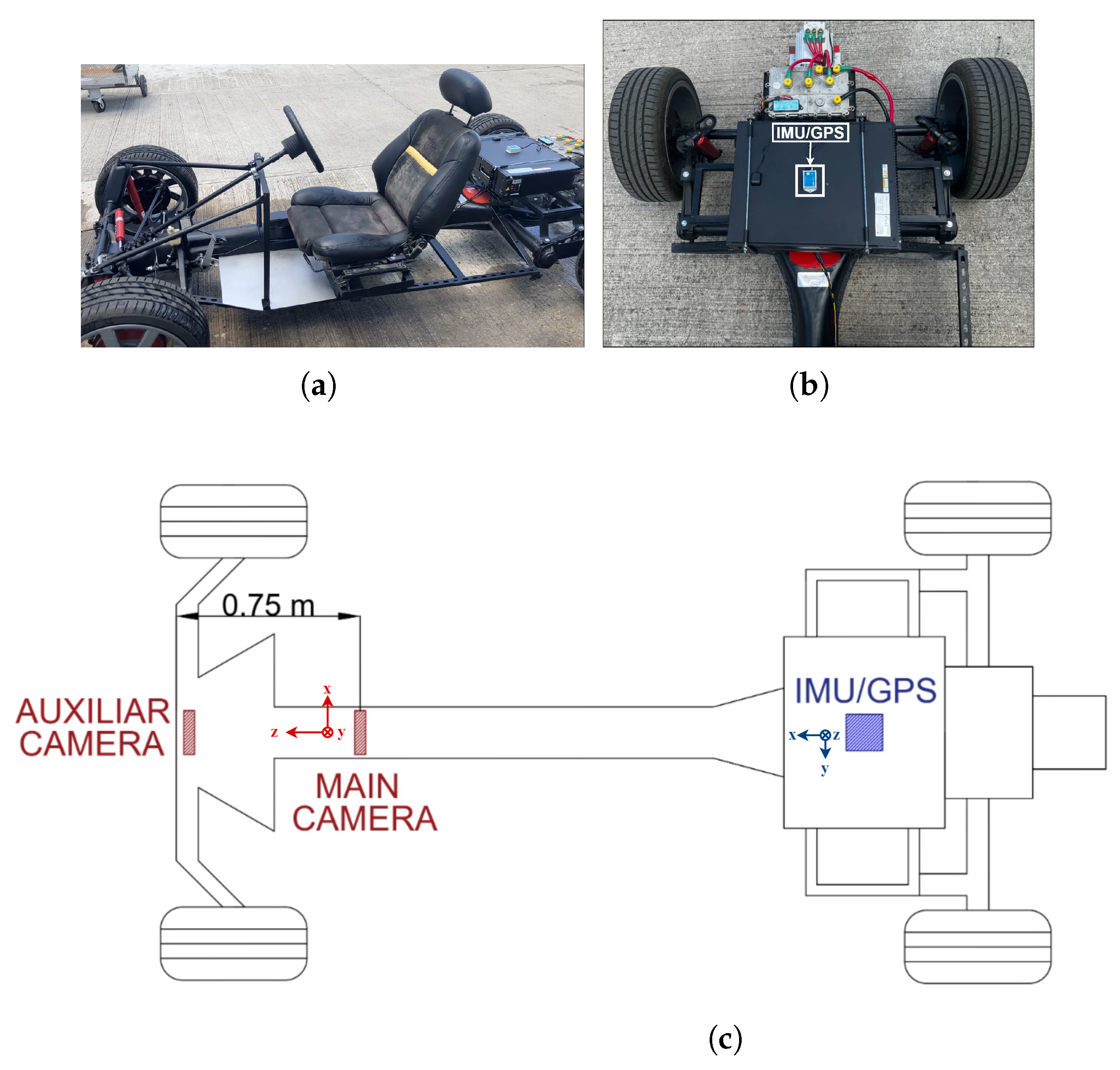
The experimental platform used for validating this proposal is illustrated in Figure 3a. This vehicle was a prototype of an electric car assembled on campus, combining new and recycled components. This electric car was 60% complete; although it achieved a velocity over 80 km/h, the battery autonomy was around 90 km under normal driving conditions, bringing stability and soft shock-absorbing. Figure 3b illustrates the car’s rear part with the IMU and GPS sensors. Additionally, this electric car was equipped with two cameras; all sensor locations are depicted in Figure 3c. Although the prototype was able to move orward and reverse, only forward movement was considered in this work.

2.2. Color and Depth Image Acquisition

The two cameras included in the electric car were Intel RealSense 400 series RGBD cameras [30]. As the schematic diagram in Figure 3c illustrates, the first camera was placed $0.75$ m to the front of the vehicle in the chassis center and on a $0.5$ m high base. This camera was considered the principal or primary camera due to its localization providing a field of view (FOV) of ${65}^{\circ }\times {40}^{\circ }$ for depth images and ${69}^{\circ }\times {42}^{\circ }$ for color images. This FOV adequately captured objects in the $0.6$ m to 3 m range in front of the vehicle. Using only the primary camera, the first $0.6$ m in front of the car remained in a blind spot. To cover that distance, an auxiliary camera was placed at the center of the vehicle’s bumper on a base of $0.3$ m high and pointing slightly downward.

The images were acquired using the Open3D library [31] in Python. The acquisition module was divided into three tasks: (1) camera recognition, (2) setting and obtaining configuration parameters, and (3) image storage and related information for the following processing stages. The first task checked the computer’s correct connection and recognition of the cameras. In the second, the parameters for image acquisition were configured. The resolution was $640\times 480$, and the acquisition frame rate was 21 fps for RGB and depth images. In addition, the intrinsic parameters of the primary camera were also calculated for the 3D point projection. These parameters were the focal length (as a multiple of pixel width and height) and the coordinates of the image’s principal point (as a pixel offset from the left and top edge). The values obtained are shown in

Table 1. Intrinsic parameters of the main camera.

Intrinsic Parameter	Values
Focal length [$f_x$, $f_y$]	[611.71044, 611.11853]
Coordinates of the image’s principal point [$p{p}_x$, $p{p}_y$]	[322.10314, 231.02186]

.

The third method included color and depth image storage; the timestamp was saved in an additional text file. Figure 4 illustrates the FOV of the color and depth images acquired from the primary camera. The depth images were stored in 16 bits. Each pixel in the depth image represented the object’s distance value in the scene, illustrated by the color image.

Five trajectories were carried out with the electric car, acquiring around 2000 color images and their corresponding depth images per trajectory. The traveled path was around 100 m long in a straight direction with vehicles on the left side of the route and safety cones on the right. All the trajectories illustrated static outdoor scenes. First, a 2D image analysis was performed, and then, the most representative points were projected to 3D space, resulting in low computational costs and reducing the quantity of the processed data. The following subsection describes the image analysis and the object region extraction to predict and validate the navigation environment.

2.3. ROI Features and Objects Point Clouds

The Oriented FAST and Rotated BRIEF (ORB) [32] is an open-source descriptor employed to detect the 2D feature points in images. ORB feature extraction is a strategy that combines FAST (features from accelerated segment test) and BRIEF (binary robust independent elementary features). FAST is a descriptor that focuses on finding the highlighted corners compared with their surrounding pixels. FAST is known for its speed, making it suitable for real-time applications. Additionally, the ORB method uses a multi-scale image pyramid to detect feature points in the image at different scales. In this case, an eight-level pyramid was selected with a scale factor of $1.2$ between each level. Conversely, BRIEF is a binary feature descriptor that generates a compact binary code for each key point. It uses pairs of pixels to create binary tests and determines whether a pixel’s intensity is greater or less than its neighbor’s. The resulting binary code concisely represents the local image patch around a critical point. After using this method, we obtained an ORB object that contains the pixel coordinates of 1500 feature points and their orientation. It was identified that in the images, an area of the sky remained constant and was not considered a region of interest. Therefore, this region was discarded in the search for the feature points. Figure 5a shows the selected area in blue and the extracted feature points within it.

The projection of points to 3D coordinates was performed using Matlab’s pcfromdepth function. This function received the pixel coordinates of the feature points, found them in the depth image, and took the depth value corresponding to each point. This value corresponded to estimating the z-coordinate of the points in the real coordinates. Some regions in the depth images contained a zero value, representing error areas or undefined zones by the infrared sensor in the Intel camera; therefore, these points were discarded. Consequently, only the points in the camera range were considered for object detection, localization, and classification. The camera had an ideal depth range of 3 m. This value could not be extended, but it was possible to adjust this 3 m range depending on the camera’s location. In this case, the working distance started at 2 m in front of the camera, so the depth range was considered from 2 to 5 m. This adjustment required a depth factor to fit the values into the new range. For the outdoor context illustrated in our experimental tests, the depth factor was set to 1400. On the other hand, the camera’s intrinsic parameters helped to obtain the real xy coordinates from the pixel coordinates. As a result, a vector containing the estimated values of the actual 3D coordinates of the valid feature points was obtained.

As mentioned above, the selected ORB points were uniformly distributed on the image, except in the zone of the sky. Under this assumption, some points were detected in the road. To keep only the points of the objects, the Simple Morphological Filter (SMRF) [33] algorithm was used to segment the point clouds into ground or nonground points. The SMRF divides the point cloud into a grid with a resolution given by the user as an input parameter to the algorithm. After setting the depth range and ground segmentation, approximately 85% of the points in Figure 5a were removed in Figure 5b. Most points were eliminated by depth range, and the remaining points were concentrated in the objects’ region. A binary mask was constructed with the ORB points location in 2D as shown in Figure 6a. A growing region task was applied around the points in the binary mask to convert the points to closed areas (see Figure 6b). Edges in the color image were extracted using a vertical Roberts kernel, illustrated in Figure 6c. The borders in Figure 6c delimited the region growing task of Figure 6b, resulting in the areas and edges shown in Figure 6d. Then, a dilation morphology process and area filters were carried out in Figure 6d, resulting in Figure 6e. This binary mask helped the areas merge with the objects in the color image to obtain a bounding box that enclosed and fitted the whole object better. The region of the objects was delimited in bounding boxes, as illustrated in red in Figure 6f.

The centroids of the bounding boxes were considered to calculate the distance from the objects to the front of the vehicle. Similarly, the coordinates of the centroids were also found in the depth image to estimate the distance in the z-axis parallel to the vehicle’s path. Instead of using only the center of the bounding box to calculate the distance from the car to the object, a $3\times 3$ matrix around this centroid was employed. Thus, the matrix average in the depth image was used as the object location.

2.4. Occupancy Map and Car Pose Estimation

Figure 7 shows one of the vehicle trajectories, which was obtained by plotting its position data from a GPS sensor. The starting point is labeled in green, and the ending point is marked in red. The vehicle navigated a trajectory of 100 m around the A and B buildings of the campus with an average velocity of 8 km/h. During image acquisition, a CSV file stored the index of the captured images and their corresponding timestamp. At the same time, the data acquired by the IMU and GPS were saved in a text file. This data included vehicle speed, geographic coordinates, and the data timestamp. Velocity data were filtered by selecting only the values higher than zero. The first velocity value, different from zero, indicated that the vehicle started to move. Similarly, the last velocity value higher than zero indicated that the navigation task ended.

The total trajectory traveled by the experimental platform was around 100 m. However, this work only described the global occupancy map’s detection, localization, and update for the first 25 m. Figure 8 shows the initial occupancy map generated from physical measurements of the distance between obstacles and their dimensions. The map was divided into $10\times 10$ cm cells, and the area occupied by the objects was represented with black regions. If this region occupied at least a small part of a cell, the entire cell was considered occupied; therefore, the occupied areas depicted on the map were slightly larger than the actual objects. Moreover, the red point on the map represented the starting point. During the navigation task, the car position is given by the GPS and compared with the vision-based object locations. The object’s positions were calculated as described in the previous section. The timestamp of the images allowed for a reinforcement during vehicle navigation because, in addition to the visual pose, the pose information could be obtained from the GPS at the same timestamp. Therefore, vision-based object detection in front of the car simultaneously with the GPS pose was also possible.

The initial map was sketched with the actual measurements of the static scenario. The vehicle started in the center of the road, which in the image map of Figure 8 was equivalent to the ($350,0$) coordinate. All measurements considered the front of the vehicle as a reference point. On the other side, the estimated map was created by converting the 3D coordinates of the points into grid coordinates using the world2grid Matlab function. Grid coordinates were projected in a binary occupancy map to obtain the estimated global map.

The image and GPS data synchronization was performed according to the timestamps stored in the CSV and Txt files. The camera captured 21 fps; however, only one image per second was processed to extract ORB features and their projection to 3D space. Furthermore, this sequence of images was used to estimate the vehicle’s position every second through the navigation task. To do this, the image acquired every second or every 21 frame was considered a keyframe. Each keyframe performed a feature match, and the difference in the features’ position helped estimate the camera’s rotation and translation employed to estimate the camera trajectory. The 3D points were adjusted according to the camera movement for each keyframe. On the other hand, the 2D feature points of each frame were projected from the local map to the global map of the navigation scene.

To validate the estimated position, geographic coordinates from GPS were transformed to Universal Transverse Mercator (UTM) coordinates using the deg2utm function to obtain $x-y$ coordinates. The distance between each pair of data poses acquired was calculated. Afterwards, the accumulated sum of distances provided the total length of the car trajectory. The distance estimated with the images through 21 frames was equivalent to the sum of the distances calculated from the GPS measurements per second. The GPS provided around 5 measurements per second.

Once the bounding boxes of the objects were calculated, these were simultaneously used as the input of a classifier based on a convolutional neural network (CNN) to identify the objects detected. The design and implementation of the classifier are explained in the following section.

2.5. CNN Architecture for Object Classification

The regions of interest extracted in the color image were assumed to contain objects of the environment. However, a reliable class could be calculated using robust deep-learning tools based on CNN models. To achieve highly accurate results, CNN requires a dataset with minimal image samples for training and validation. The classifier implemented in this work is depicted in Figure 9. The dataset contained eight categories of objects commonly found in the urban context. Then, the bounding boxes selected during the 3D feature validation stage were used as inputs to the final trained CNN to determine the label and score class prediction.

2.6. Dataset Description and Alex Net Model

The training dataset was acquired with a video camera in the rear-view mirror of a vehicle that navigated the urban center of two neighboring cities from the campus. In the first city, 10 videos were acquired in the afternoon to avoid sunshine in the camera, with a clear sky, following a route of approximately $11.5$ km, storing a total of one and a half hours of videos. Under similar weather conditions, the same recorded video duration was acquired in the second city, following a route of $13.5$ km. Templates of the predefined classes were extracted from the sequence of video images using a segmentation-based CNN model.

Object patches in

Table 2. Categories trained with the CNN architecture.

Patches	Classes	# Samples
	Bicycle	2919
	Car	3464
	Motorcycle	2651
	Pedestrian	2584
	Safety cone	3001
	Traffic sign	2900
	Tree	2681
	Truck	3236
	Total	23,436

show similar illumination conditions to the images acquired with the intel camera shown in Figure 4a. The segmentation model tested was the Fast Convolutional Neural Network (F-CNN) [34] pretrained with Common Objects in Context (COCO) model [35], using PixelLib library [36]. This network simplifies the extraction of object patches among thousands of images. As a result, every object patch shows a clean background, providing a complete and balanced training and validation dataset. The dataset comprises 23,436 image patches; 16,406 patches are used for training and 7030 for validation.

The AlexNet model was used for classifying objects during vehicle navigation with 30 training epochs. The size of the images tested was set to $227\times 227\times 3$. The Alex-Net model is composed of eight layers: five convolutional layers through Rectified Linear Unit (ReLU) activation (1, 3, 5, 6, and 7) and three fully connected layers (2, 4, and 8) with adaptative gradients like an optimizer. Finally, a softmax layer reduces the network output to eight categories. The label and score obtained by AlexNet architecture are displayed with the objects bounding box for this driving assistance proposal.

3. Results

In this section, the experimental tests performed are detailed. The image dataset was acquired in a controlled environment on a section of the campus road; there were 8 classes considered for the training the model: bicycle, car, motorcycle, pedestrian, safety cone, traffic sign, tree, and truck.

A plot of the car trajectory is illustrated in red in Figure 10. This path is the visual pose estimated by the camera on board the vehicle. The resolution of this plot was notably high, so the trajectory did not look like a straight line, illustrated by GPS data in Figure 7. Moreover, the point clouds on the left and right of the red trajectory represent the meaningful points detected in the color image and projected to the 3D space. The classification module provides a category for the objects in this part of the scene.

The comparison between the estimated position on the z-axis and the distance calculated using the IMU and GPS during 16 s of trajectory is shown in

Table 3. Difference between visual-based estimated and GPS car pose.

	Z-Axis Position (m)
Time (s)	Estimated	GPS	Error (m)	Velocity (km/h)
1	0.3722	0.3891	0.0169	2.685
2	0.8706	0.8351	0.0355	3.018
3	1.4029	1.3362	0.0667	3.333
4	2.0728	1.8901	0.1827	3.852
5	2.7595	2.5002	0.2593	4.148
6	3.4908	3.7739	0.2831	4.407
7	4.5312	4.4386	0.0926	4.592
8	5.3728	5.1216	0.2512	4.833
9	6.1267	5.8237	0.3031	4.963
10	7.0877	7.2444	0.1568	5.093
11	8.0256	8.0008	0.0248	5.259
12	8.9706	8.7759	0.1947	5.463
13	9.8779	9.5701	0.3077	5.611
14	10.9351	10.3453	0.5898	5.630
15	11.7587	11.1393	0.6194	5.667
16	13.3592	12.7629	0.5964	5.907

.

The 25 m of the traveled path corresponded to approximately 350 images acquired during 16 s. Considering the camera’s FOV, the images were cropped to $640\times 100$ pixels, excluding the sky zone in the image but keeping the essential working distance and depth of field. The reference axis for detecting and localizing the objects was set at the camera position. The traveled distance of the car was obtained according to the GPS data and was compared with the visual-based estimated trajectory. Table 3 shows that the minor error found in the distances was $0.0169$ m, while the largest was $0.6194$ m. Additionally, the table shows a trend of a higher error as the speed of the car increased. Note that most visual estimated distances were greater than those calculated with GPS. Nevertheless, the error between GPS and visual data car pose could be neglected because object detection and localization using visual data were the main goals for achieving car navigation. The object was detected near its current position, enough to advise the car system about potential objects.

Because of the feature points partially covering the object surface, obtaining a bounding box enclosing it was complex. The color image was preprocessed to improve the bounding box described in Section 2.3. From the 3D points obtained, a 2D projection was created using the X and Z coordinates of the points to construct an estimated occupancy map. Figure 11 shows the intersection between this map and the initial occupancy map. The green areas in the figure represent the actual occupied position in the initialized map, and the pink areas represent occupied cells in the estimated map. In contrast, black areas represent the intersected areas in the maps. Note that the estimated map areas intersected the initial map at least with a small part, but enough to validate the object’s presence. The red point in Figure 11 is the starting point of the car trajectory. The safety cones were on the right of the car path for each tested environment. It is observed that the estimated position of the cones was slightly ahead of the real one. Furthermore, another difference between the initial and visual estimated maps was the size of the objects detected. Despite the difference, the occupied cells represented all the objects in the route.

Classification Results

The AlexNet architecture was trained considering a holdout process of 70% for training and 30% for validation during 30 epochs, using the dataset described in Table 2. Figure 12 shows an accuracy of $96.87$% during the training process. At the tenth epoch, the model’s performance began a stable behavior with a performance above 90%.

Moreover, the confusion matrix in Figure 13 achieved an accuracy of $85.66$% and shows the detailed classification results for each category. Note that the categories with similar patterns, like a bicycle with a motorcycle and a car with a truck, showed higher confusion errors. Similar errors were achieved for three additional datasets from the electric vehicle navigating an outdoor scene containing cars, trucks, trees, and safety cones. The datasets showed the highest classification error for cars and trucks. The classification error increased when the bounding box partially extracted the original object. On the contrary, objects fully enclosed in the bounding box were correctly classified with a high estimation score.

Table 4. Evaluation metrics.

Class	Precision	Recall	F1-Score
Bicycle	92.29%	82.07%	86.88%
Car	74.44%	76.80%	75.60%
Motorcycle	85.44%	90.06%	87.69%
Pedestrian	88.16%	88.40%	88.28%
Safety cone	96.18%	89.55%	92.75%
Traffic sign	83.91%	97.12%	90.03%
Tree	93.08%	93.78%	93.43%
Truck	77.00%	72.09%	74.46%

presents the Precision, Recall, and F1-score metrics for the dataset described in Table 2. The trained model showed a reliable performance for eight classes. The number of images in the dataset for the bicycle, car, motorcycle, and truck classes could reduce the error bias by increasing the number of samples and previously eliminating samples in conflict [37].

Figure 14 illustrates eight images extracted from the navigation task for $t=0$, 3, 5, 9, 13, 27, 32, and 48 s. These images illustrate the bounding boxes of the classified objects, the label and the predicted score assigned by the classifier, and the distance estimated to the electric car. When $t=3$, 13, and 32, the feature points were not detected in the safety cone region; therefore, the conditions for generating the bounding box of this object were insufficient. By analyzing the depth value close to the image margin, the depth value was less than 2 m, being out of range for the infrared camera. Thus, the objects in this zone of the image are missed. In contrast, in the remaining images in Figure 14, the number of feature points was enough, and the depth value was inside the detection range; thus, the bounding box could be calculated for object classification and pose prediction in the scene.

4. Discussion

The proposed visual navigation method is developed for an electrical car navigating in an outdoor controlled environment delimited by safety cones on the right side and cars parked on the left side of the path. Given an initial global map, the vehicle goes straight on the road, acquiring visual and pose information from two cameras, as well as IMU and GPS in a static scene. Five navigation sequences are obtained for distinct locations of the objects in the path. Thus, the experimental datasets for testing and validating our proposed strategy were acquired at different times during a sunny day. All the objects in the camera’s detection range were generally detected, located, and classified accurately. For instance, most of the safety cones were seen, considering that the camera was moving at 8 km/h, and the object locations were good enough to advertise the vehicle about the presence of obstacles. Moreover, including vehicle pose from the IMU was our second reference value to reinforce vehicles and object visual pose. The resolution of the occupancy map allowed for the inclusion of minor objects, although cars were the most common objects around the route.

By validating the GPS car location versus visual-pose estimation illustrated in Table 3, it can be noticed that the errors found every second could be neglected regarding the objects and car dimensions. That is, 20 or even 30 cm of error was low considering the car’s dimensions and the mandatory safety zone around the obstacles during car navigation. Considering that the smaller objects on the road were around 45 cm, the error obtained was minimal in the obstacle safety zones. Moreover, in Figure 10, the most significant 3D feature points were plotted as point clouds located to the right and left of the car’s trajectory to represent the occupied zones in the environment. However, the practical side of this work allowed the occupied area to be calculated slightly behind its current location. In the worst case, the error pose indicated to the vehicle that the object was still in an earlier position, even if the object had currently fallen around it. The objects’ dimensions in the navigation environment were significant; therefore, detecting the objects with an average accuracy was enough to advise the vehicle about potential obstacles in the route.

Like our proposed research, in [9], the authors presented a multi-sensor fusion to estimate the vehicle’s trajectory utilizing an odometer, IMU, and vision camera for vehicle localization, achieving a low MSE score when comparing the pose estimation. However, multi-sensor (GNSS, IMU LiDAR and visual camera) approaches require high processing and power demands, as demonstrated in [24]. In contrast, our work used GPS and an RGB-D sensor for vehicle localization in exclusive lanes, dealing with fewer processing and synchronization requirements.

5. Conclusions

The challenges faced by driverless vehicles can be resolved by developing fast and accurate strategies to deal with unpredictable environments or situations. Although the development of autonomous cars has been largely explored, this field is still open to new embedded, feasible, and reproducible approaches for experimental and practical vehicles. This work proposed a visual-based object detection and localization module for assisting the navigation of an electric car. Color and depth images were analyzed and combined to extract 2D features and project the corresponding point clouds. By detecting the feature points in the road, these were eliminated from the 3D points, with only the points belonging to objects remaining. A bounding box containing the object feature points in the color image was extracted and classified by a CNN. The overall strategy allowed for the extraction of feature objects to calculate their estimated pose regarding the camera for constructing the visual-estimated occupancy map. This map was validated with the global occupancy map of the navigation path. The resulting occupancy map had an error of 20 to 60 cm regarding the object pose provided in the initial map. However, the obtained error was low considering the object’s dimensions and the mandatory safety zone around the obstacles during car navigation. Moreover, the detected and located objects were accurately classified using an AlexNet model. Thus, the occupied cells of the map were labeled with known objects. Although navigation strategies were proposed for static environments, the visual estimated map helped the vehicle generate a path, providing a first module for assisting our experimental platform.

Future works aim to enhance the generalization of our method for different navigation environments. First, we will include dynamic objects in the environment, such as people, cars, or cyclists. We will program and instrument high-speed graphical processing cards on board the vehicle. Additionally, we will include an embedded stereo camera for real-time visual analysis and to quantitatively measure the estimation error.