AI-Driven Prediction and Mapping of Soil Liquefaction Risks for Enhancing Earthquake Resilience in Smart Cities

Abstract

In response to increasing urbanization and the need for infrastructure resilient to natural hazards, this study introduces an AI-driven predictive model designed to assess the risk of soil liquefaction. Utilizing advanced ensemble machine learning techniques, the model integrates geotechnical and geographical data to accurately predict the potential for soil liquefaction in urban areas, with a specific focus on Yokohama, Japan. This methodology leverages comprehensive datasets from geological surveys and seismic activity to enhance urban planning and infrastructure development in smart cities. The primary outputs include detailed soil liquefaction risk maps that are essential for effective urban risk management. These maps support urban planners and engineers in making informed decisions, prioritizing safety, and promoting sustainability. The model employs a robust combination of artificial neural networks and gradient boosting decision trees to analyze and predict data points, assessing soil susceptibility to liquefaction during seismic events. Notably, the model achieves high accuracy in predicting soil classifications and N-values, which are critical for evaluating soil liquefaction risk. Validation against an extensive dataset from geotechnical surveys confirms the model’s practical effectiveness. Moreover, the results highlight the transformative potential of AI in enhancing geotechnical risk assessments and improving the resilience of urban areas against natural hazards.

1. Introduction

In an era of rapid urbanization and escalating environmental challenges, the concept of ‘smart cities’ as shown in Figure 1 has emerged as a pivotal framework for sustainable development [1,2,3,4]. These cities harness advanced technologies, such as IoT and big data analytics, to enhance quality of life, economic efficiency, and environmental sustainability [5]. A key element of this initiative is the integration of artificial intelligence (AI) into urban planning processes [6]. This integration not only revolutionizes resource management in urban areas but also enhances their resilience against natural hazards like earthquakes, torrential rain, and so on [7]. This study leads in applying smart technologies in geotechnical engineering, enhancing urban resilience through AI-driven risk prediction and zoning for soil liquefaction risk. By leveraging sophisticated AI algorithms to analyze extensive geotechnical data, this methodology facilitates the creation of detailed hazard maps. These maps are indispensable for effective urban planning and hazard mitigation, equipping urban planners and engineers with essential tools to make informed decisions that prioritize safety and sustainability.

The increasing frequency of urban hazards poses significant risks to densely populated areas, highlighting the critical importance of this study. By leveraging predictive analysis, smart cities can proactively address these challenges, ensuring preparedness and adaptability within a dynamic urban environment. This study significantly enhances conventional methods by delivering a nuanced, precise, and dynamic evaluation of soil liquefaction risks, particularly in regions sensitive to geological and topographical variations. Moreover, the smart city design strategy outlined in this study encompasses comprehensive urban development, incorporating strategic infrastructure placement, optimized resource management, and improved citizen engagement through transparent data practices. By integrating AI-driven tools into the urban fabric, we ensure that cities are not only functional but also resilient and responsive to the needs of their inhabitants. The introduction of such advanced technological solutions tackles long-standing urban challenges and aligns with the broader objectives of smart cities. The predictive capabilities developed in this study represent a significant advancement in protecting and enhancing urban livability, marking a critical contribution to the conceptualization and design of smart cities worldwide.

This study focuses on the significant natural hazard of soil liquefaction, as illustrated in Figure 2 and Figure 3 [8,9,10,11,12]. Figure 3, taken from the 2011 Great Japan Earthquake, the largest recorded earthquake in Japan’s history, shows particularly severe liquefaction. This figure shows the ground devastation caused by liquefaction, including toppled trees and the flooding of streets with swirling muddy water in the Urayasu residential area [13]. As a representation of liquefaction damage, Figure 3 highlights the frequent seismic activity in Japan, which often results in severe ground instability. The risk of liquefaction occurs when five specific conditions are met: the fine particle content of the soil is between 15% and 50%; water is present; the soil is loosely compacted; the particle sizes are uniform; and the area has experienced repeated earthquakes. Soil liquefaction primarily occurs due to the shaking of loosely packed, water-saturated soils during earthquakes. This shaking increases pore water pressure and reduces the effective stress between soil particles, leading to fluid-like soil behavior, as depicted in Figure 2. Notable events, such as the 2011 Great East Japan Earthquake and the 2024 Noto Peninsula Earthquake, highlight the devastating impacts of these phenomena and underscore the critical need for accurate prediction and effective mitigation strategies [7].

This study utilizes AI algorithms to predict risks associated with soil liquefaction by analyzing extensive datasets from geological surveys and seismic activity. The choice was made to use an ensemble method over a single machine learning approach. According to [14], in geological prediction studies, the ensemble method can yield a 20% improvement in model performance, demonstrating greater potential. Therefore, the goal is to develop an AI-driven predictive model that integrates various databases, including geotechnical and geographic information, using ensemble machine learning techniques. This model specifically aims to predict potential risks of soil liquefaction, with a particular focus on areas like Yokohama, Japan, which is known for its extensive reclaimed lands and high susceptibility to these hazards. By creating and validating hazard maps through case studies in such regions, the study aims to enhance urban planning and significantly contribute to the development of smart cities.

Yokohama is located in the Tokyo metropolitan area. Originally, it was planned to use construction debris from large-scale developments to fill the land, but in reality, most of the fill material consisted of sand from Mt. Asama. According to earthquake data for the past 30 days, Yokohama has experienced seven earthquakes of magnitude 1 or greater. Therefore, the liquefaction hazard in Yokohama is considered serious. Figure 4 summarizes past earthquake-induced liquefaction damage by topographic classification, which divides the country into grids approximately 250 m square. Each grid is classified into five levels to indicate the relative intensity of liquefaction susceptibility based on general ground characteristics as represented by the topography. However, this does not predict specific earthquake-induced liquefaction events.

In the integration and visualization of the smart city concept illustrated in Figure 5, an AI-driven predictive model that synthesizes data from diverse databases, including geotechnical and geographic information, enhances urban resilience and promotes the development of a safer and more sustainable society. This approach contributes to the sustainable growth of smart cities and ensures the safety of their inhabitants. In smart cities, prioritizing the reduction of natural hazard risks is crucial. The AI-driven predictive model leverages geo-information databases to assess liquefaction risks, minimizing potential damage to buildings and infrastructure during earthquakes. The model’s high accuracy enables the identification of specific areas at risk of liquefaction, allowing for the proactive planning of effective countermeasures. Such capabilities expedite and streamline disaster responses, diminishing disruptions during emergencies. Additionally, this method provides a more detailed and accurate risk analysis than traditional approaches reliant on human judgment, thereby enhancing scientific decision-making in the planning and development within smart cities.

In this study, the authors develop a novel AI-driven predictive model that substantially advances the state of the art in assessing soil liquefaction risks, particularly in urban areas prone to seismic activity. Unlike previous studies [15,16,17,18], which primarily employed empirical or semi-empirical methods, this AI-driven model utilizes advanced ensemble machine learning techniques to integrate comprehensive geotechnical and geographic data. This integration yields a more precise, dynamic, and detailed assessment of soil liquefaction risks. The model is distinct in its ability to synthesize data from multiple sources, including real-time geological surveys and seismic records, thereby enhancing the accuracy of risk mapping and the efficacy of urban planning strategies. Moreover, the AI-driven predictive model addresses a critical gap in existing methodologies [15,16,17,18] by providing high-resolution hazard maps that are crucial for enhancing urban resilience in smart cities. By conducting a comparative analysis with models described in recent studies [15,16,17,18], this study not only fills a vital knowledge gap by improving the granularity and accuracy of predictions but also broadens the application of AI in geotechnical engineering, setting a new benchmark for future study and practical applications in earthquake-prone urban environments.

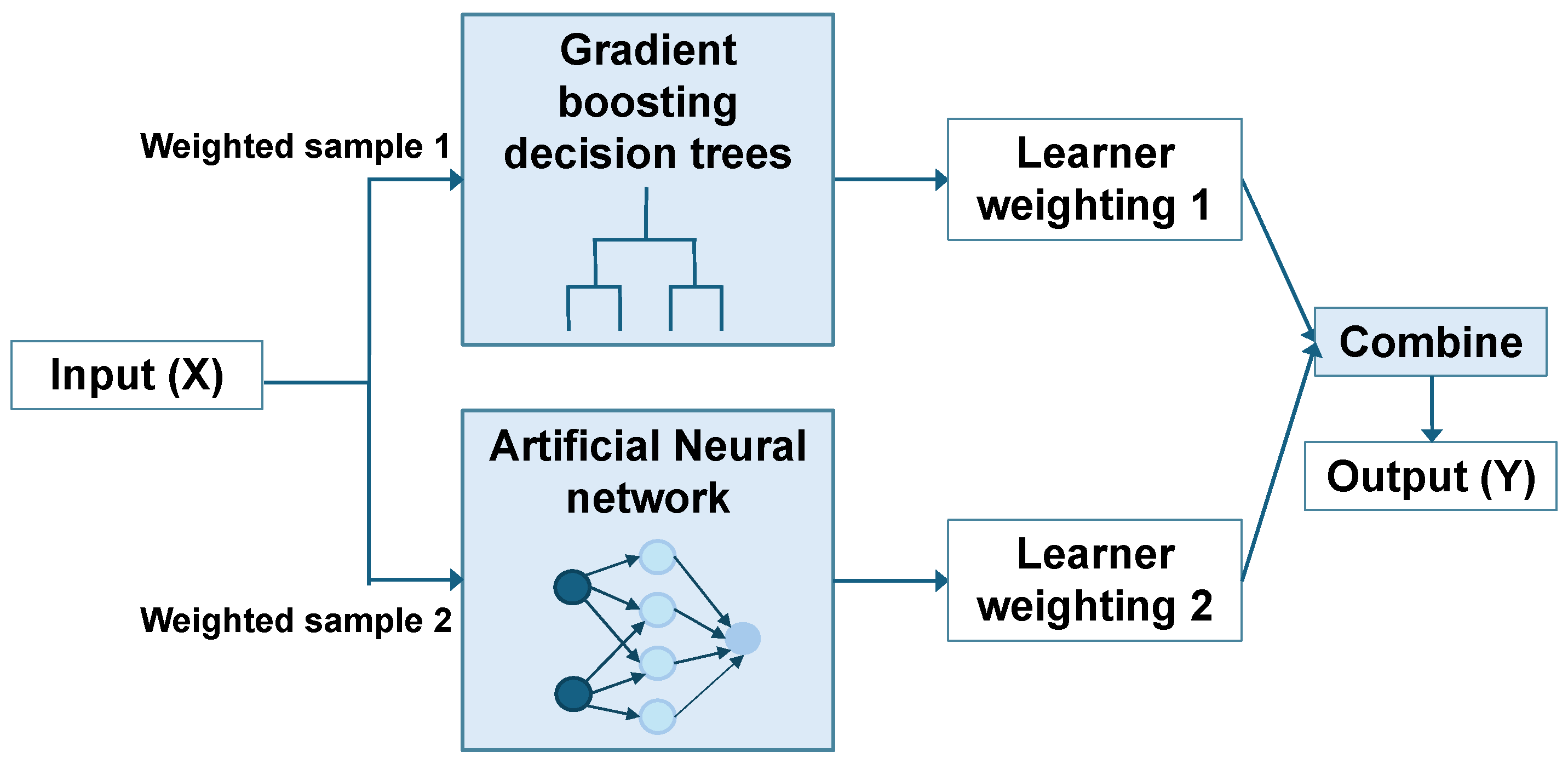
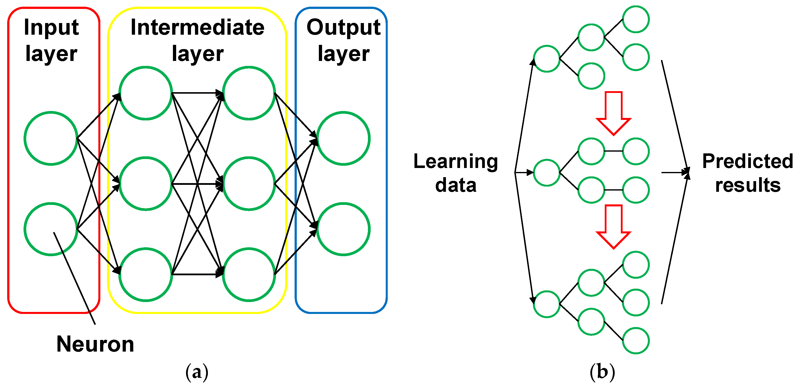
2. AI-Driven Predictive Models

In statistics and machine learning, ensemble machine learning trains multiple machine learning models (algorithms) and combines their predictions to obtain improved performance and better generalization ability than individual models. The fundamental idea behind ensemble machine learning is the recognition that each machine learning model has limitations and can make errors. Hence, ensemble machine learning aims to improve classification performance by harnessing the strengths of multiple models. Limitations of some machine learning models include high variance, high bias, and low accuracy [19,20]. However, several studies have shown that ensemble machine learning often achieves higher accuracy than a single machine learning model [21]. Ensemble machine learning can limit the variance and bias errors associated with a single model; for example, ensemble machine learning with a bagging algorithm reduces variance without increasing bias, while ensemble machine learning with a boosting algorithm reduces bias [22,23,24]. Overall, ensemble machine learning is more robust than an individual machine learning model [25]. Algorithms used in ensemble machine learning are mainly divided into three categories: bagging, boosting, and stacking. In this study, the boosting algorithm was selected for ensemble machine learning.

2.1. Ensemble Machine Learning

Boosting is an algorithm that sequentially fits “weak” classifiers to different weightings of the observations in a dataset. Those observations, that the previous classifier poorly predicts, receive greater weight in the next iteration. The final classifier is a weighted average of all the weak classifiers. In a wide variety of problems, the weighting scheme and final classifier of the boosting algorithm are merged, and the result has proven to be an effective method for reducing bias and variance.

The ensemble machine learning model is established using a boosting algorithm, and the procedure is illustrated in Figure 6, where sample data are randomly extracted from the training dataset. In this study, ensemble machine learning with the boosting algorithm was adopted, and an AI-driven predictive model was created by integrating a neural network with a gradient boosting decision trees model. By combining the strengths of different machine learning models, it is possible to achieve higher prediction accuracy than with a single model.

An artificial neural network model as shown in Figure 7a is a soft computing technique used today by engineers around the world for a wide variety of nonlinear problems that can occur in civil engineering [26]. And it is an interconnected collection of simple processing elements, units or nodes, whose functionality is loosely based on the animal neuron. The processing capability of the network is stored in the inter-unit connection strengths or weights, which are obtained through a process of adaptation to, or learning from, a set of training patterns [27,28]. Recently, artificial neural networks achieved outstanding results in learning image representations for various vision tasks, including image classification [29] and object detection [30]. These artificial neural networks typically consist of several components, including convolutional, fully connected, and pooling layers. By stacking several of these layers, convolutional artificial neural networks are able to learn complex features that are highly invariant and discriminative [31]. Previous studies confirmed it as the most suitable and widely accepted statistical approach for soil liquefaction assessment [32,33].

A gradient boosting decision trees model shown in Figure 7b is a powerful machine learning tool that is widely used in many applications, including multi-class classification. This model uses decision trees as the base algorithm and sums the predictions of a series of trees. At each step, a new decision tree is trained to fit the residual errors between the ground truth and the current prediction. Gradient boosting decision trees are popular due to their accuracy, efficiency, and interpretability [34].

In the ensemble machine learning model, the tuning of hyperparameters plays a critical role in optimizing model performance. Hyperparameters in ensemble algorithms, such as the number of base algorithms, the learning rate, and the depth of decision trees, require careful calibration to balance the tradeoff between bias and variance, thereby improving the generalizability of the model. The process of hyperparameter tuning involves a systematic search for the optimal settings that maximize the predictive accuracy of the ensemble. Techniques such as grid search, random search, and Bayesian optimization are commonly used for this purpose. These methods effectively explore the hyperparameter space and identify configurations that lead to the best performance on validation data sets. In this study, random search was employed to optimize model performance within the ensemble machine learning framework.

The main reason for choosing ensemble learning is the limited size and uneven distribution of the data set, which consists of only 214 data points, as shown in Figure 8. Ensemble learning is used to improve the accuracy and reliability of predictions. This method generates training sets by randomly drawing small samples from all categories and combining them with larger samples from the same categories. This process is repeated several times to create different training sets and models. Finally, a combination method, such as voting or weighted voting, is used to produce the classification predictions. Thus, when big data research methods are faced with data scarcity, the ensemble approach is chosen to increase accuracy.

2.2. Reliability of Predictive Results by AI-Driven Predictive Model

In order to evaluate the performance of the AI-driven predictive model, “Accuracy”, “Coefficient of determination ($R^2$)”, “Average Precision (AP)”, “Average Recall (AR)”, and “F-measures” are selected as evaluation indicators.

“Accuracy” is the most basic index and is an evaluation index that indicates the percentage of correctly predicted predictions. This study calculated the “Accuracy” using Equation (1) [35,36] and the “Accuracy” was used as an evaluation index for predicting soil classification in this study:

$$Accuracy={\displaystyle \frac{TP+TN}{TP+FN+FP+TN}}$$

(1)

where, $TP$ is true positives, $TN$ is true negatives, $FP$ is false positives, and $FN$ is false negatives.

“Coefficient of determination ($R^2$)” [37] is a key evaluation metric in predictive modeling. It quantifies the proportion of the variance in the dependent variable that is predictable from the independent variables. $R^2$ is bounded above by 1, which indicates a perfect fit. Although there is no theoretical lower bound, a value of 0 suggests that the model predicts as well as the mean of the dependent variable, represented by the horizontal line $y=K$, where $K$ is the mean of the target values of all training points. Values of $R^2$ less than 0 indicate a fit worse than this trivial model. Consequently, $R^2$ values are typically considered within the range of 0 to 1. The coefficient of determination remains unchanged under linear transformations of the scale of measurement for the independent variables. A value close to 1 indicates a model with high predictive accuracy. $R^2$ was calculated using Equation (2):

$$R^2=1-{\displaystyle \frac{\sum _i{(y_i-x_i)}^2}{\sum _i({y_i-\overline{y})}^2}}$$

(2)

where, $y_i$ is the measured value, $x_i$ is the predicted value, and $\overline{y}$ is the average of measured values.

“Average Precision (AP)” is a comprehensive metric used to evaluate model precision across various “Intersection over Union (IoU)” thresholds. Precision assesses whether all detected positive samples are indeed positive. The steps to calculate precision accuracy are as follows: 1. establish different IoU thresholds; 2. calculate the accuracy at each IoU threshold; 3. compute the average of these accuracies. Average precision was determined using Equation (3):

$$Precision={\displaystyle \frac{TP}{TP+FP}}$$

(3)

“Average Recall” is a comprehensive metric that evaluates the recall rate of the model across different IoU thresholds. Recall measures the proportion of actual positive samples that the model correctly identifies. The steps to calculate average recall are as follows: 1. establish different IoU thresholds; 2. calculate the recall rate at each threshold; 3. compute the average of these recall rates. Recall was determined using Equations (4):

$$Recall={\displaystyle \frac{TP}{TP+FN}}$$

(4)

The “F-measure” is the harmonic mean of precision and recall. The F-measure was calculated using Equation (5):

$$\mathrm{F}\text{-}\mathrm{m}\mathrm{e}\mathrm{a}\mathrm{s}\mathrm{u}\mathrm{r}\mathrm{e}=2\times {\displaystyle \frac{Precision\times Recall}{Precision+Recall}}$$

(5)

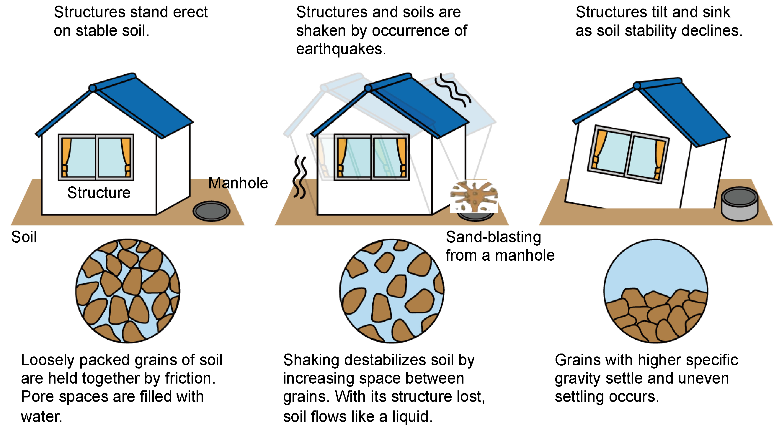
3. Soil Liquefaction Risk Prediction with AI-Driven Predictive Model

3.1. Procedures on Soil Liquefaction Risk Prediction

In this study, data from the geological columnar section provided by the Ministry of Land, Infrastructure, Transport and Tourism, accessible through their online database, was utilized for the target location, Yokohama, Japan.

Data pertaining to “N-value”, “soil classification”, and “groundwater levels” were collected from the geological columnar section for a total of 214 locations, as depicted in Figure 8. Additionally, “elevation” data were obtained from the Geospatial Information Authority of Japan, using location information. An example of these collection records is shown in Figure 9. The criteria for determining soil liquefaction, according to the Highway Bridge Specifications and Commentary, are as follows:

(1)

The groundwater level must be within 10 m of the ground surface, and saturation must occur within 20 m of the ground surface.

(2)

The fine particle content (FC) must exceed 35%, with a plasticity index of 15 or less.

(3)

The average grain size (D₅₀) must be 10 mm or less, and the 10% grain size (D₁₀) must be 1 mm or less.

The AI-driven predictive model identifies layers with an N-value of 50 or more extending over at least 2 m as indicative of a bearing layer. Generally, soil or rock with an N-value of 20 or more is considered suitable as a load-bearing layer. If the N-value is between 30 and 50, the layer is deemed appropriate for the load-bearing layer of civil engineering and building structures. An N-value of 50 or more suggests a very solid layer, suitable as a load-bearing layer capable of supporting large structures such as high-rise condominiums. Therefore, in this study, continuous strata with an N-value exceeding 50 over a length of more than 3 m are designated as load-bearing layers [38].

Major soil classification systems in Japan have evolved in conjunction with public works projects [39,40]. In Japan, soils with similar properties are grouped based on their particle size distribution. This study categorizes “soil type classifications,” derived from geological columnar sections, into five categories: sand and gravel with fine content of 35% or less (prone to soil liquefaction), and silt, clay, and bedrock with fine content of 50% or more. Additionally, when multiple soil types, such as sandy silt or sandy clay mixed with gravel, are encountered, they are classified according to the component with the largest mass proportion, following the engineering classification method for soil materials.

Concerning “groundwater levels,” the geological columnar section contained sparse data, making it impractical to gather the necessary information for predictive analysis. Consequently, the borehole water level was assumed to represent the groundwater level, which was uniformly set at GL-1.0 m.

Soil liquefaction risk is assessed for layers that satisfy the previously mentioned criteria. The AI-driven predictive model was trained using the data on “N-value” and “soil classification” to predict these parameters at unknown locations. The predicted data was then incorporated into the soil liquefaction potential index (LPI) to assess the risk of soil liquefaction.

3.2. Assumed Earthquake Motions for Soil Liquefaction Risk Prediction

Level 1 earthquake motion refers to lower-intensity seismic events that structures are expected to withstand without significant damage, typically maintaining operational functionality post-event. In contrast, Level 2 earthquake motion pertains to higher-intensity events. Buildings are designed to endure these, possibly sustaining some structural damage, to ensure occupant safety.

Regulations require consideration of two specific types of Level 2 earthquake ground motions: Type I for large plate-boundary earthquakes and Type II for inland earthquakes, such as the 1995 Hyogoken–Nanbu Earthquake. Type I earthquake motion is characterized by shorter duration and higher frequency vibrations, commonly experienced in regions close to tectonic plate boundaries. Conversely, Type II earthquake motion involves longer duration and lower frequency vibrations, typically occurring in areas more distant from plate boundaries. This classification into Types I and II aids in designing structures tailored to the specific seismic risks associated with the frequency and duration of ground shaking typical of a region.

3.3. Soil Liquefaction Potential Index

The soil liquefaction potential index ($LPI$) was utilized for analysis of soil liquefaction risk in this study. $LPI$, introduced in 1982, serves as a metric to assess the potential for soil liquefaction at a site, with higher values indicating greater risk. This index aggregates the factor of safety against liquefaction ($F_L$ value), which is weighted by depth, to evaluate the overall likelihood of soil liquefaction occurring at various depths within a site. A series of case studies applied the $LPI$ to assess liquefaction risks at targeted locations [39,40,41,42].

The $F_L$ value, essential for predicting soil liquefaction, quantifies the resistance to liquefaction at each depth. When the $F_L$ value is 1.0 or less, the occurrence of soil liquefaction is deemed likely. In this study, the $LPI$ was calculated using Equations (6)–(19) to comprehensively determine the risk of soil liquefaction at the study site:

$$LPI={\int }_0^{20}F\times (1-0.5x)d_x$$

(6)

$$F=\left\{\begin{array}{c}1-F_L(F_L<1.0)\\ 0 (F_L\ge 1.0)\end{array}\right.$$

(7)

$$F_L={\displaystyle \frac{R}{L}}$$

(8)

where, x represents the depth (m) from the ground surface; $F$ is the soil liquefaction resistance factor, which is governed by the factor of safety against soil liquefaction ($F_L$), R is the dynamic shear strength ratio, and L represents the earthquake shear stress ratio. R is determined based on the standards for Level 1 and Level 2 earthquake motions:

$$R=C_W\times R_L$$

(9)

In the case of Level 1 and Type I of Level 2 earthquake motions:

$$C_W=1.0$$

(10)

In the case of Type II of Level 2 earthquake motion:

$$C_W=\left\{\begin{array}{c} 1.0 (R_L\le 0.1)\\ 3.3R_L+0.67 ({0.1<R}_L\le 0.4)\\ 2.0 \left({0.4<R}_L\right)\end{array}\right.$$

(11)

$$R_L=\left\{ \begin{array}{c} 0.0882\sqrt{(0.85N_a+2.1)/1.7} (N_a<14)\\ 0.0882\sqrt{N_a/1.7}+1.6\times {10}^{-6}\times {\left(N_a-14\right)}^{4.5 }(N_a\ge 14)\end{array}\right.$$

(12)

In the case of sand:

$$N_a=cFC\times \left(N_1+2.47\right)-2.47 (D_{50}<2 mm)$$

(13)

$$N_1=170N/({{\sigma }_{vb}}^{\prime }+70)$$

(14)

$$C_{FC}=\left\{\begin{array}{c} 1 (0\%\le FC<10\%)\\ (FC+20)/30 (10\%\le FC\le 40\%)\\ (FC-16)/12 (40\%\le FC)\end{array}\right.$$

(15)

In the case of gravel:

$$N_a=\left\{1-\right.\left.0.36{\mathrm{l}\mathrm{o}\mathrm{g}}_{10}\times \left({\displaystyle \frac{D_{50}}{2}}\right)\right\}{N}_1(D_{50}\ge 2 mm)$$

(16)

$${L=r}_d{k}_{hgL}{{\sigma }_v{/\sigma }_v}^{\prime }$$

(17)

$$r_d=1.0-0.015x$$

(18)

$$k_{hgL}=C_Z{k}_{hgL0}$$

(19)

where, the explanation and definition of each coefficient and variable symbol used in Equations (6)–(19) are summarized in

Table 1. Explanation and definition of each coefficient and variable symbol used in Equations (6)–(19).

Coefficient and Variable Symbol	Explanation and Definition
$C_W$	Correction coefficient based on earthquake motion characteristics
$R_L$	Liquefaction strength ratio
$N$	N-value obtained from standard penetration test
$N_1$	N-value converted to effective overburden pressure equivalent to 100 (kN/m2)
$N_a$	Corrected N-value considering the effect of grain size
${{\sigma }_{vb}}^{\prime }$	Effective overburden pressure at depth from ground surface when performing standard penetration tests (kN/m2)
$C_{FC}$	Correction factor for N-value based on fine particle content
$FC$	Fine particle content (%) (Percentage of passing mass of soil particles with a particle size of 75 μm or less)
$D_{50}$	50% particle size (mm)
$r_d$	Depth reduction factor of seismic shear stress ratio
$k_{hgL}$	Design horizontal seismic intensity of the ground surface used to assess liquefaction (rounded to two decimal places)
$C_Z$	Regional correction factor (Yokohama is 1.0)
$k_{hgL0}$	Standard value of horizontal seismic intensity for design of ground surface used to judge liquefaction
${\sigma }_v$	Total overburden pressure at depth x from ground surface (kN/m2)
${{\sigma }_v}^{\prime }$	Effective overburden pressure at depth x from ground surface (kN/m2)
$X$	Depth from ground surface (m)

.

Table 2. Correction coefficients based on the characteristics of earthquake motion.

Type of Site	Level 1 Earthquake Motion	Level 2 Earthquake Motion
		Type I	Type II
Site I	0.12	0.5	0.8
Site II	0.15	0.45	0.7
Site III	0.18	0.4	0.6

presents the correction coefficients based on the characteristics of earthquake motion.

Table 3. Physical properties of different soil types related to existing groundwater.

Soil Classification	Unit Weight of Soil Below Groundwater Table (kN/m3)	Unit Weight of Soil Above Groundwater Table (kN/m3)	FC (%)
Clay	13	15	80
Silt	15.5	17.5	75
Sand	18	20	10
Gravel	19	21	0
Bedrock	20	20	5

details the physical properties of different soil classifications related to existing groundwater.

When the $LPI$ equals 0, the risk or potential for soil liquefaction is very low. For 0 < $LPI$ ≤ 5, the risk or potential is low; for 5 < $LPI$ ≤ 15, it is high; and for $LPI$ > 15, it is very high.

Table 4. Correlation between liquefaction potential index (LPI) and liquefaction risk levels.

	0 < LPI < 5	0 < LPI < 15	15 < LPI < 30	LPI > 30
Liquefaction risk	Very low	Low	High	Very high

summarizes the correlation between $LPI$ and liquefaction risk levels.

4. Results and Discussion

This study concentrates on geotechnical data derived from the geological columnar sections of Yokohama. Here, an AI-driven predictive model is employed to forecast the distribution of N-values and soil classifications. Case 1 involves predicting N-values, while Case 2 focuses on predicting soil classifications.

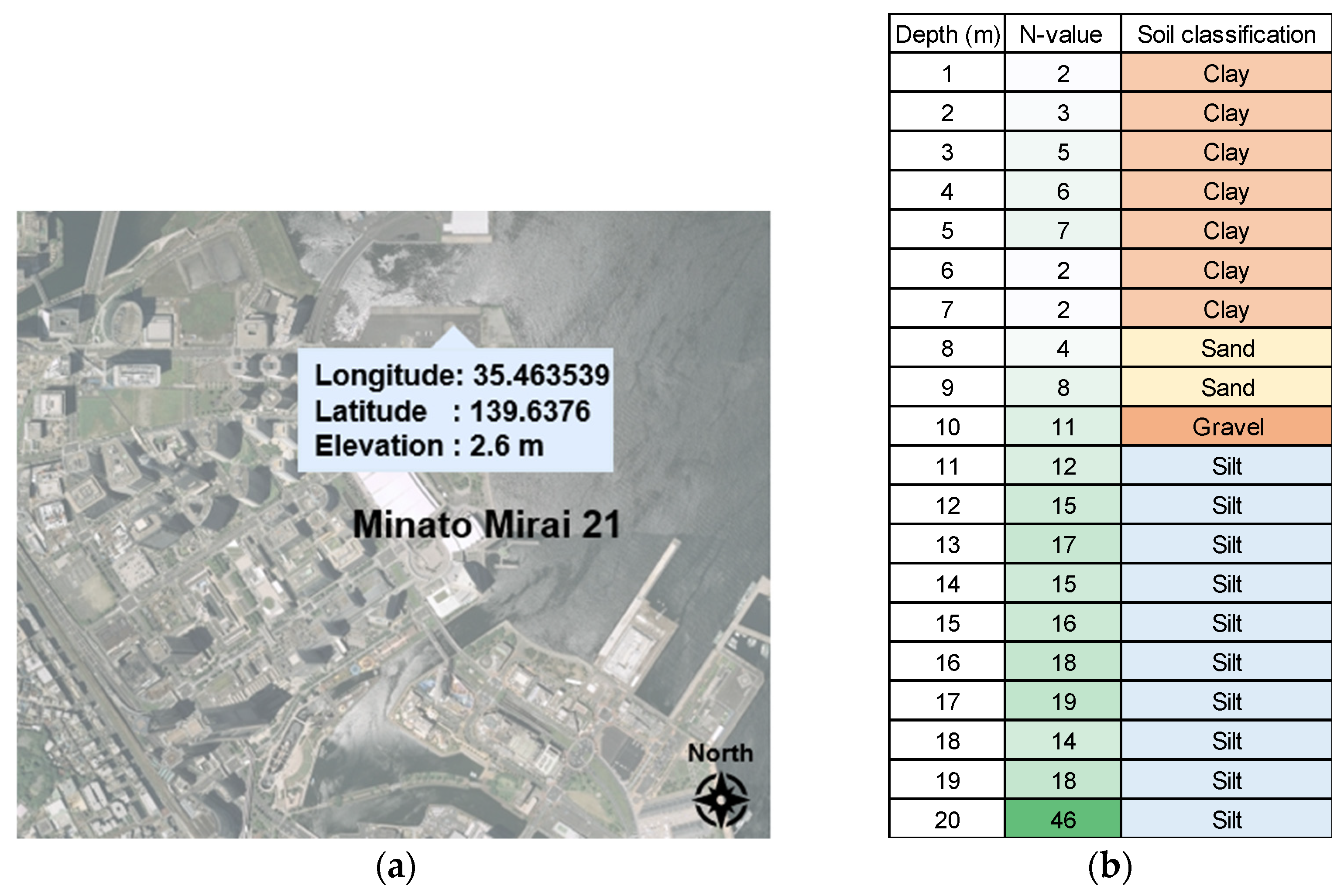
4.1. N-Values and Soil Classification Predictions

4.1.1. Case 1: Predictive Results for N-Value

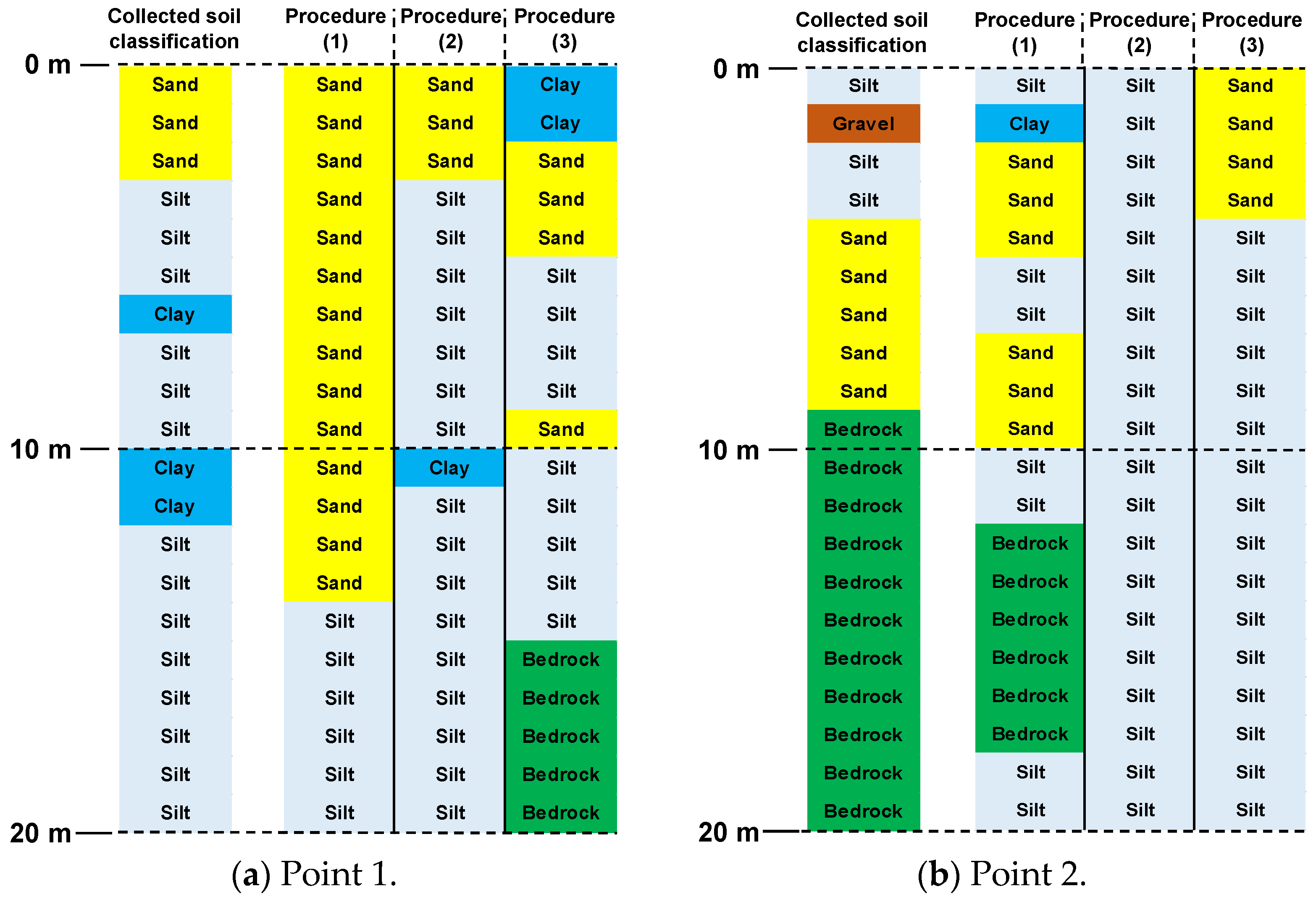
Using geotechnical data collected from the geological columnar sections of Yokohama as training data, the AI-driven predictive model estimated the N-value at sites previously assumed to be unknown, though they were actually known.

To compare prediction accuracy based on data volume, the model’s performance was evaluated at 214 sites and at half that number. Model 1 used data from 117 sites, while Model 2 used data from all 214 sites. The data set is divided into a training set, a test set, and a validation set in proportions of 60%, 20%, and 20%, respectively. In Model 1, the training set contains 70 values, the validation set contains 24 values, and the test set contains 23 values. In model 2, the training set contains 140 values, the validation set contains 48 values, and the test set contains 46 values.

Table 5. Coefficient of determination ($R^2$) for predicting N-value.

(a) Model 1.			(b) Model 2.
Depth (m)	Coefficient of Determination (R2)	Root Mean Square Error (RMSE)	Depth (m)	Coefficient of Determination (R2)	Root Mean Square Error (RMSE)
1	0.0114	7.32	1	0.0720	6.38
2	0.0487	6.22	2	0.0695	7.67
3	0.0254	8.82	3	0.4005	8.65
4	0.2626	6.61	4	0.7248	6.18
5	0.2086	8.15	5	0.7445	7.00
6	0.4704	8.31	6	0.4879	11.13
7	0.2557	8.92	7	0.5324	12.09
8	0.6190	8.39	8	0.8231	8.23
9	0.7429	8.52	9	0.8096	9.21
10	0.6894	9.90	10	0.5211	15.14
11	0.6581	11.14	11	0.8628	8.29
12	0.9339	5.44	12	0.9112	6.80
13	0.9097	6.71	13	0.9518	5.72
14	0.9030	7.04	14	0.8981	7.46
15	0.9085	7.21	15	0.9314	6.18
16	0.8915	7.91	16	0.9763	3.63
17	0.9458	5.63	17	0.9379	5.90
18	0.8969	7.74	18	0.9130	6.87
19	0.8924	7.89	19	0.9168	6.73
20	0.8083	10.52	20	0.9063	7.11

shows the coefficient of determination ($R^2$) for predicting the N-value in Model 1 and Model 2, respectively. From the evaluation results for the N-value, it was observed that this tends to increase with increasing depth. This may be attributed to the increasing number of points (load-bearing layer) where the N-value exhibits a consistent range of fluctuation at greater depths, and the range of N-values at these points becomes narrower. Therefore, it can be inferred that predictions in deeper ground can be made with relatively high accuracy. Comparing prediction accuracy based on the number of data points reveals that the accuracy of the N-value predictions improves as the number of points increases. By gathering more data points to create training data, more reliable and precise predictions can be expected.

Therefore, Model 2 was selected for prediction. The N-value was predicted using data from 214 sites in Yokohama. Given the differing geologies of reclaimed land and plateaus, Yokohama was categorized into two types: ‘Landfill area (red)’ and ‘Plateau area (blue)’. Areas assumed to be unknown points were distinguished from known points in each category. Point 1 was selected from the landfill area and Point 2 from the plateau area, with their locations illustrated in Figure 8. Additionally, this study predicted the N-value, assumed to be an unknown point, using the following three prediction procedures. The method that achieved the highest accuracy was selected:

(1)

A prediction procedure involving learning at every 1 m interval, without using the prediction results as data.

(2)

A prediction procedure that makes predictions at every 1 m interval from the ground surface to the subsurface, incorporating prediction results shallower than the predicted depth into the learning process.

(3)

A prediction procedure that makes predictions at every 1 m interval from 20 m below ground to the surface, incorporating prediction results deeper than the predicted depth into the learning process.

Figure 10 shows the results of predicting the N-value using each of the prediction procedures (1) to (3). Looking at the results for Point 1, while the results show that the N-value is low, prediction procedures (1) and (2) show that the N-value is 30 or more from points 10 m onwards. This is because the number of collected geotechnical data for a total of 214 points is more in the plateau area than in the landfill area, and there is much data that reaches the load-supporting layer from points around 10 m or higher and converges to an N-value of 30 or more. It is thought that this is having an influence. On the other hand, with prediction procedure (3), although the numerical value exceeds the survey results, it appears that similar behavior is predicted at points beyond 10 m while maintaining a relatively low N-value. As a result, at Point 1, prediction procedure (3) is more accurate than (1) and (2). Next, looking at the results for Point 2, all prediction procedures showed behavior similar to the survey results, and it can be said that predictions were made with relatively high accuracy. Among them, prediction procedure (3) can also predict the tendency of the survey N-value at a depth of around 5 m, and it is clear that the overall prediction accuracy is higher than (1) and (2). Based on the results of Points 1 and 2, it is thought that the prediction procedure (3) is better at making predictions at large depths because it learns and makes predictions from underground. Based on the above results, the following step was taken in this study: the prediction procedure (3) was chosen for prediction.

4.1.2. Case 2: Predictive Results of Soil Classification

Similar to Case 1, geotechnical data collected from the geological columnar sections of Yokohama were utilized as training data to develop the AI-driven predictive model for soil classification. The results of the model’s prediction accuracy are displayed in

Table 6. Predicted accuracy for predicting soil classification.

(a) Model 1.					(b) Model 2.
Depth (m)	Accuracy (%)	Average Precision (%)	Average Recall (%)	F-Measure (%)	Depth (m)	Accuracy	Average Precision (%)	Average Recall (%)	F-Measure (%)
1	90.10	77.38	55.65	75.19	1	79.34	77.61	61.77	79.34
2	87.13	84.49	53.85	72.65	2	81.13	81.62	62.59	82.32
3	85.15	80.69	60.98	80.65	3	79.44	79.53	49.67	81.03
4	88.89	91.97	77.7	82.91	4	86.45	85.92	66.89	84.22
5	84.16	81.9	80.06	80.8	5	84.91	82.12	78.82	79.6
6	86.14	87.34	82.8	84.65	6	85.92	82.86	67.55	83.57
7	84.00	79.43	79.66	79.50	7	82.71	60.26	62.21	76.51
8	86.00	76.32	70.86	71.89	8	84.58	80.01	64.47	79.93
9	86.00	76.32	70.86	71.89	9	84.51	78.93	65.76	79.75
10	75.25	74.73	59.96	61.92	10	85.51	78.17	75.29	75.99
11	87.13	81.13	71.12	73.64	11	93.46	92.19	88.94	90.35
12	85.15	82.01	75.21	77.56	12	88.79	85.85	84.88	84.9
13	93.07	87.65	80.89	82.62	13	88.79	93.64	97.12	69.8
14	93.00	94.84	79.84	83.64	14	94.34	92.05	80.54	84.13
15	93.94	95.96	75	77.92	15	94.84	97.29	76.71	82.83
16	91.00	93.47	56.27	77.47	16	95.33	86.63	71.23	87.76
17	94.74	91.03	91.63	91.25	17	94.31	85.97	82.56	83.92
18	84.16	67.23	52.86	72.31	18	94.37	91.73	76.38	93.48
19	88.12	93.91	60.61	64.81	19	96.26	96.25	95.46	95.81
20	87.13	86.35	60.08	64.26	20	95.79	95.94	92.95	94.33

. Accuracy metrics were employed to assess the model’s performance. The results indicate high accuracy starting from a depth of 1.2 m, suggesting that predictions are generally reliable. Observations show that surface-near points are predominantly sandy, and as depth increases, the load-bearing layer is encountered more frequently, and the presence of bedrock points increases, which correlates with improved accuracy. In addition, prediction accuracy improves as the number of data points increases. The accuracy of the model was evaluated using four metrics: accuracy, average precision, average recall, and the F-measure.

In addition, the three prediction procedures of (1) to (3) used for N-value estimation were also applied to predict soil classification at unknown points. The results are detailed in Figure 11. According to these tables, the results at Point 1 show that the soil type, as identified from geotechnical data gathered from geological columnar sections, is characterized as sand up to about 3 m deep and silt below this depth. Furthermore, the geotechnical data reveal intermittent clay layers from 8 m to 15 m deep, which prediction procedures (1) and (2) failed to detect. In contrast, the prediction procedure (3), which analyzes data from deeper layers upwards, successfully predicted the presence of clay with relative accuracy.

For Point 2, mixed soil types are observed up to 10 m depth, beyond which the soil reaches the load-bearing layer and is identified as bedrock. The predictions accurately reflected the mixed soil types up to 10 m; however, they deviated from the geotechnical data at certain depths, resulting in less accurate classifications. At depths greater than 10 m, prediction procedures (1) and (2) predicted only silt and failed to identify the bedrock. This discrepancy is likely due to the dataset predominantly classifying the ground that reaches the load-bearing layer as silt rather than bedrock. However, akin to its performance at Point 1, the prediction procedure (3) successfully predicted the presence of bedrock layers and mixed soil types below 10 m with greater accuracy. Consequently, the prediction procedure (3) was chosen for further soil classification predictions in this study.

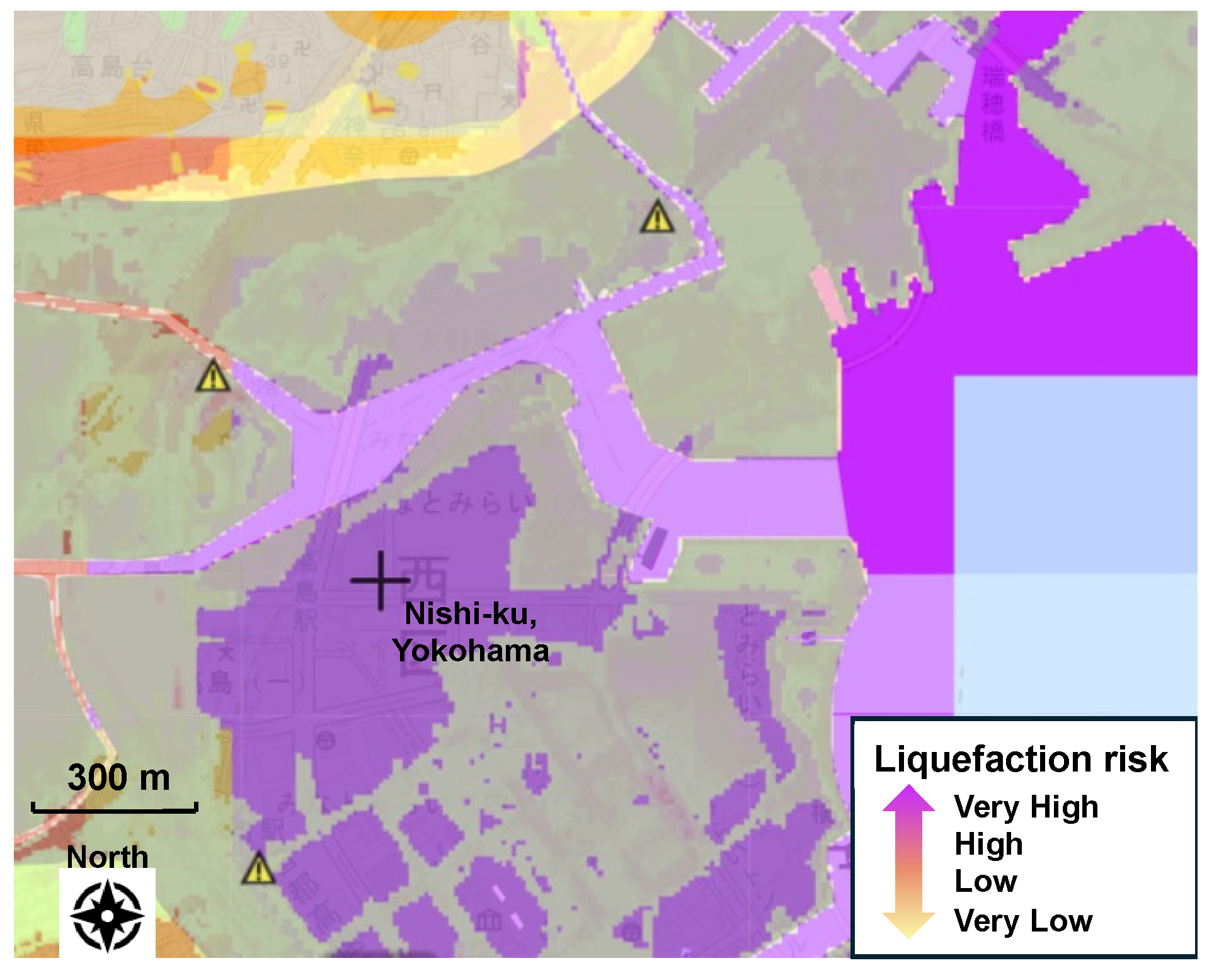
4.2. Creation of Soil Liquefaction Risk Mapping

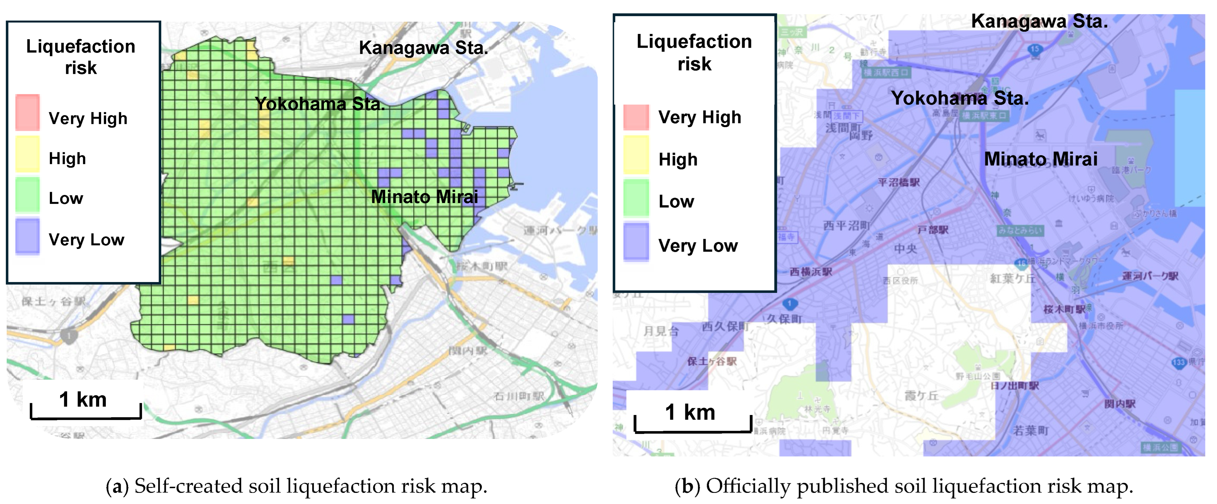
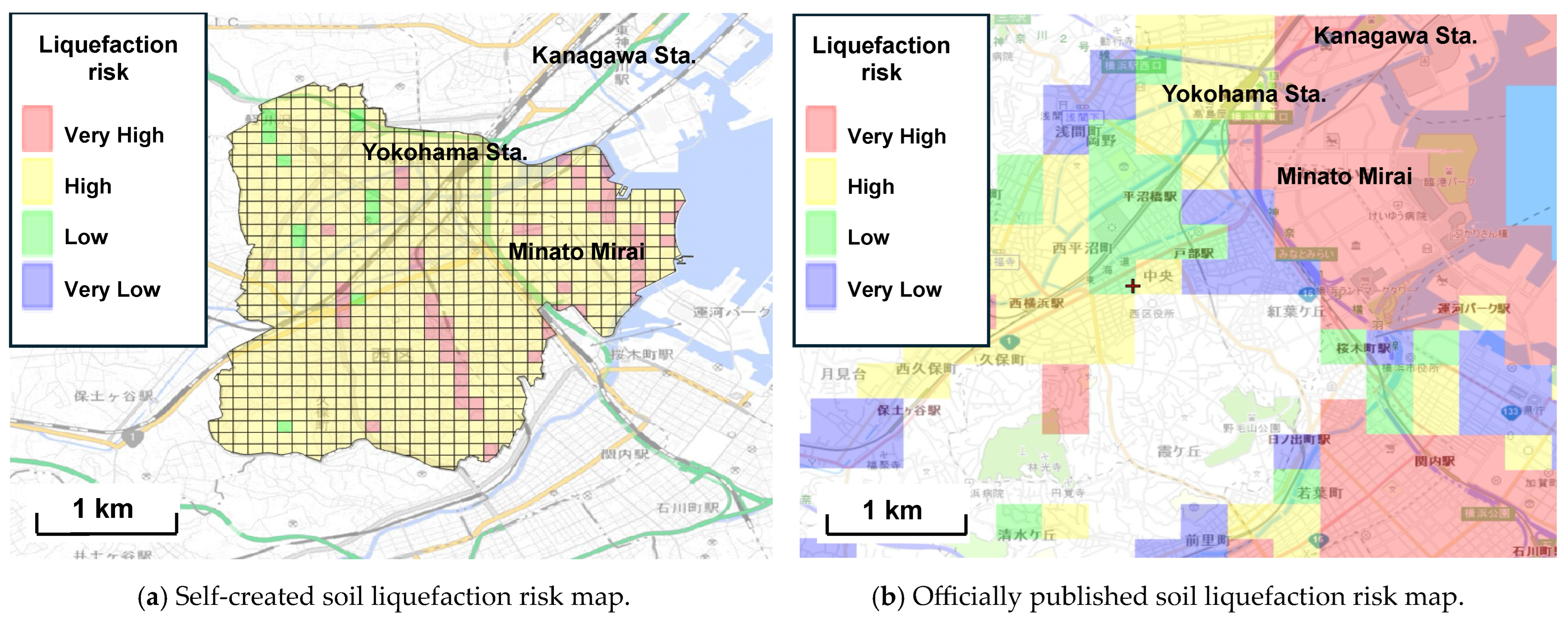
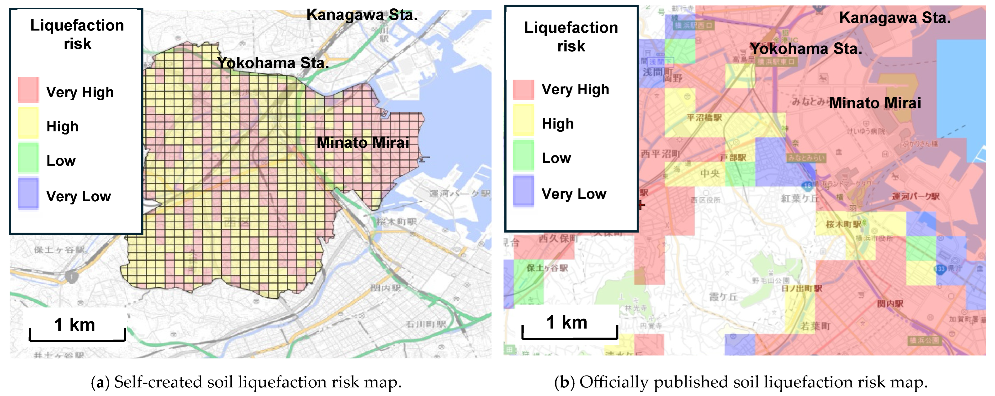
4.2.1. Comparison of Self-Created and Existing Soil Liquefaction Risk Maps

During the site selection and planning stages for engineering structures and human settlements, the soil liquefaction potential of an area is a critical factor considered in geotechnical engineering. Accurately evaluating the soil liquefaction potential is the first step towards mitigating soil liquefaction hazards. Soil liquefaction risk maps have been prepared by many autonomous bodies in Japan to assess the impact of soil liquefaction in each target area [43,44,45,46]. These maps are essential tools in the development of smart cities, where resilient urban planning and infrastructure are paramount. By integrating these hazard maps into urban planning processes, smart cities can optimize their development strategies to enhance safety and sustainability in earthquake-prone areas.

The creation of these maps can generally be divided into three steps: The first step involves calculating the spatial distributions of the instrumental seismic intensity for ten recent earthquakes that resulted in soil liquefaction. In the second step, the results of these seismic intensity distributions are compared with liquefied sites from past earthquakes to estimate the ratio of soil liquefaction occurrence. The third step involves merging geomorphological classes with similar soil liquefaction susceptibilities and applying a regression method to estimate the final probability of soil liquefaction occurrence based on instrumental seismic intensity.

Unlike previous approaches [15,16,17,18], this study first makes predictions for unknown locations and then uses these results to create hazard maps. Soil liquefaction risk maps were developed for three types of earthquake motions. Level 1 earthquake motion refers to seismic activity that is likely to occur once or twice during the lifespan of a structure; however, the intensity of such shaking is relatively low and is not expected to damage the structure. Figure 12a displays a self-created soil liquefaction risk map for Level 1 earthquake motion, while Figure 12b depicts the official soil liquefaction risk map for the same level published by Yokohama. These maps feature a 100 m × 100 m grid and are color-coded according to the soil liquefaction risk. Conversely, Level 2 earthquake motion represents a seismic event that is less likely to occur but could be extremely severe, potentially causing significant damage. This level is subdivided into Type I, which anticipates a major earthquake at the plate boundary, and Type II, which considers an inland earthquake. Figure 13a shows a self-created soil liquefaction risk map for Level 2 earthquake motion with Type I, while Figure 13b shows the official soil liquefaction risk map for the same level and type published by Yokohama. Figure 14a shows a self-created soil liquefaction risk map for Level 2 earthquake motion with Type II, while Figure 14b shows the official soil liquefaction risk map for the same level and type published by Yokohama. The two prediction models differ primarily in their variables. While the existing official map of soil liquefaction risk is based solely on terrain differentiation, our self-generated map incorporates additional variables beyond terrain differentiation.

The soil liquefaction risk maps created in this study reveal a relatively larger area at high risk of soil liquefaction compared to the maps published by Yokohama. Another major advantage of using AI models is the ability to quickly update maps as new geotechnical information and seismic data become available. This is a time-consuming task using standard methods, but can be done efficiently using AI. The maps created in this study were divided into detailed risk levels, making it easier to develop countermeasures for each level of risk. The highly accurate maps created by AI will provide important information to local residents and governments, helping them to formulate specific action plans to improve the safety of local communities. This is expected to minimize damage in the event of a liquefaction disaster. It can be confirmed that the liquefaction risk maps created in this study have many advantages over the existing maps provided by Yokohama. This will enable safer and more accurate disaster planning and further improve preparedness for future disasters.

However, the model developed in this study exhibits significant limitations. First, the training dataset is inadequate, comprising just over 200 data points, which is insufficient for most machine learning algorithms that require large datasets to function effectively. This constitutes a major limitation. Second, the representativeness of the training data is questionable. As illustrated in Figure 7, the data distribution is quite dispersed, potentially compromising the model’s generalization capability. Therefore, a critical step for future development is to acquire more comprehensive data, ideally exceeding 500 data points. A literature review [7] identified a dataset that includes latitude, longitude, elevation, and ‘n’ values for 433 data points in Tokyo, which could provide a basis for enhancing the data pool and refining the model.

4.2.2. Advantage of Soil Liquefaction Risk Maps Created by AI-Driven Predictive Model

The integration of AI into soil liquefaction risk prediction and mapping represents a transformative development in geotechnical engineering, particularly within the framework of smart cities. This paper explores the advantages of using AI-driven predictive models to produce detailed and dynamic soil liquefaction risk maps, enhancing urban resilience to earthquakes and other seismic activities. AI-driven predictive models represent a significant advancement over traditional liquefaction risk assessment methods, which typically rely on historical data and empirical formulas. While useful, traditional methods often fail to capture the complex, dynamic interactions within urban environments or adapt to rapid changes in urban landscapes. In contrast, AI models can continuously learn and adapt by integrating multiple data sources, including real-time geotechnical, geographic, and seismic data. This integration allows for a more nuanced and accurate assessment of liquefaction risk, providing urban planners and engineers with powerful tools for proactive urban development and disaster mitigation.

As shown in

Table 7. Advantages of AI-driven liquefaction risk maps to improve urban planning, safety, and sustainability in smart city.

Advantage	Description
Dynamic Updates	The AI-driven predictive model can continuously update and refine predictions as new data become available, which is critical in rapidly changing urban areas.
Adaptability	The AI-driven predictive model adapts to changes in the urban landscape, such as construction and land use changes, maintaining the accuracy and relevance of risk maps.
Complex Data Analysis	The ability of the AI-driven predictive model to process large data sets enables the analysis of complex variables and interactions, providing more detailed and comprehensive risk assessments.
Emergency Preparedness	The AI-driven predictive model guides emergency planning and response efforts, improving resource allocation and response times during seismic events.
Proactive City Planning	Prediction of potential liquefaction zones helps to avoid building in high-risk areas or to implement special construction techniques to mitigate risk.
Support for Smart Cities	Integrates with smart city goals to improve sustainability, safety, and quality of life by applying advanced technology to urban planning.
Enhanced Urban Resilience	Improves resilience to earthquakes and seismic activity, contributing to safer and more sustainable urban environments.

, one of the key advantages of AI-driven liquefaction risk maps is their ability to dynamically update and refine predictions as new data become available. This capability is critical in urban areas where conditions can change rapidly due to construction, land use changes, and environmental factors. AI models can adapt to these changes, maintaining the accuracy and relevance of risk maps. Additionally, AI ability to process large datasets enables the analysis of complex variables and interactions that would be too time-consuming or impossible for traditional methods, resulting in more detailed and comprehensive risk assessments. Another significant advantage of AI-driven hazard maps is their contribution to emergency preparedness and response strategies. Detailed hazard maps created from AI predictions can guide emergency planning and response efforts, helping to allocate resources more efficiently and improve response times during crises. For example, during an earthquake, AI-driven maps can quickly identify areas most at risk of soil liquefaction, allowing emergency services to prioritize these areas for immediate attention. In addition, these AI-driven maps facilitate better urban planning and infrastructure development. By predicting potential liquefaction zones, city planners can avoid building critical infrastructure in high-risk areas or implement special construction techniques to mitigate the risks. This proactive approach not only saves costs associated with repairing damage after a disaster but also protects lives by reducing the risk of catastrophic failure during seismic events.

The advantages of soil liquefaction risk maps created by AI-driven predictive models are numerous and significant. They provide a more accurate, detailed, and adaptive tool for managing geotechnical risk in urban environments. These maps enhance urban planning, improve emergency preparedness, and contribute to the overall resilience and sustainability of cities. As urban areas continue to grow and face complex challenges, the role of AI in geotechnical engineering will become increasingly important, marking a pivotal shift toward more intelligent, responsive, and resilient urban environments.

5. Conclusions

In this study, a self-developed AI-driven predictive model was trained to analyze geotechnical data collected from geological columnar sections at known points to predict the ‘N-value’ and ‘soil classification’ at unknown points. The predicted data were then used in the liquefaction potential index (LPI) to assess soil liquefaction risk and to create maps for various levels of seismic motion. The findings include the following:

(1)

It was confirmed that the larger the training dataset used in the AI-driven predictive model, the higher the accuracy of the predictions.

(2)

The prediction procedure, which estimates the N-value and soil classification from 20 meters below ground to 1 meter above ground and incorporates learning from results deeper than the predicted depth, was found to be the most accurate.

(3)

The AI-driven predictive model provided more detailed soil liquefaction risk mapping for the seismic motion level compared to existing mappings.

Future challenges include enhancing prediction accuracy. Despite utilizing the most accurate procedure available in this study, the predictions were not entirely consistent, with some demonstrating low accuracy due to biases in the training data. Further data collection, exploration of data processing methods, combinations of explanatory variables, and the development of new prediction techniques are necessary. In terms of assessing trigger risks, further improvements in prediction accuracy and the exploration of new evaluation methods may facilitate the creation of more precise hazard maps. Beyond assessing risks associated with soil liquefaction, this methodology could feasibly be applied to comprehensively evaluate other hazard risks and to generate maps predicting potential damage from various hazards.

References

1. Trindade, E.P.; Hinnig, M.P.F.; Costa, E.M.D.; Marques, J.S.; Bastos, R.C.; Yigitcanlar, T. Sustainable development of smart cities: A systematic review of the literature. J. Open Innov. Technol. Mark. Complex. 2017, 3, 1–14. [Google Scholar] [CrossRef]
2. Sharifi, A.; Allam, Z.; Bibri, S.E.; Garmsir, A.R.K. Smart cities and sustainable development goals (SDGs): A systematic literature review of co-benefits and trade-offs. Cities 2024, 146, 104659. [Google Scholar] [CrossRef]
3. Su, Y.; Fan, D. Smart cities and sustainable development. Reg. Stud. 2023, 57, 722–738. [Google Scholar] [CrossRef]
4. Mishra, R.K.; Kumari, C.L.; Krishna, P.S.J.; Dubey, A. Smart cities for sustainable development: An overview. In Smart Cities for Sustainable Development; Springer: Singapore, 2022; pp. 1–12. [Google Scholar] [CrossRef]
5. Ismagilova, E.; Hughes, L.; Dwivedi, Y.K.; Raman, K.R. Smart cities: Advances in research—An information systems perspective. Int. J. Inf. Manag. 2019, 47, 88–100. [Google Scholar] [CrossRef]
6. Cugurullo, F.; Caprotti, F.; Cook, M.; Karvonen, A.; Guirk, P.M.; Marvin, S. The rise of AI urbanism in post-smart cities: A critical commentary on urban artificial intelligence. Urban Stud. 2024, 61, 1168–1182. [Google Scholar] [CrossRef]
7. Cong, Y.; Inazumi, S. Integration of smart city technologies with advanced predictive analytics for geotechnical investigations. Smart Cities 2024, 7, 1089–1108. [Google Scholar] [CrossRef]
8. Cong, Y.; Motohashi, T.; Nakao, K.; Inazumi, S. Machine learning predictive analysis of liquefaction resistance for sandy soils enhanced by chemical injection. Mach. Learn. Knowl. Extr. 2024, 6, 402–419. [Google Scholar] [CrossRef]
9. Hazout, L.; Zitouni, Z.E.A.; Belkhatir, M.; Schanz, T. Evaluation of static liquefaction characteristics of saturated loose sand through the mean grain size and extreme grain sizes. Geotech. Geol. Eng. 2017, 35, 2079–2105. [Google Scholar] [CrossRef]
10. Bao, X.; Ye, B.; Ye, G.; Zhang, F. Co-seismic and post-seismic behavior of a wall type breakwater on a natural ground composed of liquefiable layer. Nat. Hazards 2016, 83, 1799–1819. [Google Scholar] [CrossRef]
11. Bao, X.; Jin, Z.; Cui, H.; Chen, X.; Xie, X. Soil liquefaction mitigation in geotechnical engineering: An overview of recently developed methods. Soil Dyn. Earthq. Eng. 2019, 120, 273–291. [Google Scholar] [CrossRef]
12. Nakao, K.; Inazumi, S.; Takahashi, T.; Nontananandh, S. Numerical simulation of the liquefaction phenomenon by MPSM-DEM coupled CAEs. Sustainability 2022, 14, 7517. [Google Scholar] [CrossRef]
13. Ishihara, K.; Araki, K.; Toshiyuki, K. Liquefaction in Tyoko Bay and Kano Regions in the 2011 Great East Japan Earthquake. Earthq. Geotech. Eng. Des. 2013, 28, 93–140. [Google Scholar]
14. Wang, Z.Z.; Hu, Y.; Guo, X.F.; He, X.G.; Kek, H.; Ku, T.; Goh, S.H.; Leung, C.F. Predicting Geological Interfaces using Stacking Ensemble Learning with Multi-scale Features. Can. Geotech. J. 2022, 60, 1036–1054. [Google Scholar] [CrossRef]
15. Kajihara, K.; Okuda, H.; Kiyota, T.; Konagai, K. Mapping of liquefaction risk on road network based on relationship between liquefaction potential and liquefaction-induced road subsidence. Soils Found. 2020, 60, 1202–1214. [Google Scholar] [CrossRef]
16. Honda, K.; Takeyama, T.; Tachibana, S.; Iizuka, A. Liquefaction risk assessment in the 23 wards of Tyoko using elastoplastic analysis. Int. J. Geomate 2021, 21, 48–54. [Google Scholar] [CrossRef]
17. Matsuoka, M.; Wakamatsu, K.; Hashimoto, M.; Midorikawa, S. Evaluation of liquefaction potential for large areas based on geomorphologic classification. Earthq. Spectra 2015, 31, 2375–2395. [Google Scholar] [CrossRef]
18. Karimzadeh, S.; Matsuoka, M. A weighted overlay method for liquefaction-related urban damage detection: A case study of the 6 September 2018 Hokkaido eastern Iburi earthquake, Japan. Geosciences 2018, 8, 487. [Google Scholar] [CrossRef]
19. Mishra, S.; Shaw, K.; Mishra, D.; Patil, S.; Kotecha, K.; Kumar, S.; Bajaj, S. Improving the accuracy of ensemble machine learning classification models using a novel bit-fusion algorithm for healthcare AI systems. Front. Public Health 2022, 10, 858282. [Google Scholar] [CrossRef]
20. Sun, Y.; Li, Z.L.; Li, X.W.; Zhang, J. Classifier selection and ensemble model for multi-class imbalance learning in education grants prediction. Appl. Artif. Intell. 2021, 35, 290–303. [Google Scholar] [CrossRef]
21. Wu, H.; Levinson, D. The ensemble approach to forecasting: A review and synthesis. Transp. Res. Part C Emerg. Technol. 2022, 132, 103357. [Google Scholar] [CrossRef]
22. Doroudi, S. The bias-variance tradeoff: How data science can inform educational debates. AERA Open 2020, 6, 4. [Google Scholar] [CrossRef]
23. Ghosal, I.; Hooker, G. Boosting random forests to reduce bias; One-step boosted forest and its variance estimate. J. Comput. Graph. Stat. 2020, 30, 493–502. [Google Scholar] [CrossRef]
24. Alelyani, S. Stable bagging feature selection on medical data. J. Big Data 2021, 8, 11. [Google Scholar] [CrossRef]
25. Miemye, I.D.; Sun, Y. A Survey of ensemble learning: Concepts, algorithms, applications, and prospects. IEEE Access 2022, 10, 99129–99149. [Google Scholar] [CrossRef]
26. Ghnai, S.; Kumari, S.; Jaiswal, S.; Sawant, V.A. Comparative and parametric study of AI based models for risk assessment against soil liquefaction for high intensity earthquakes. Arab. J. Geosci. 2022, 15, 1262. [Google Scholar] [CrossRef]
27. Zhong, L.; Guo, X.; Xu, Z.; Ding, M. Soil properties: Their prediction and feature extraction from the LUCAS spectral library using deep convolutional neural networks. Geoderma 2021, 402, 115366. [Google Scholar] [CrossRef]
28. Pham, B.T.; Nguyen, M.D.; Ly, H.B.; Pham, T.A.; Hoang, V.; Le, V.H.; Le, T.T.; Nguyen, H.Q.; Bui, G.L. Development of artificial neural networks for prediction of compression coefficient of soft soil. In Proceedings of the 5th International Conference on Geotechnics 2020, Civil Engineering Works and Structures, Hanoi, Vietnam, 31 October–1 November 2019; Springer: Singapore, 2020; pp. 1167–1172. [Google Scholar]
29. He, K.; Zhang, X.; Ren, S.; Sun, J. Deep residual learning for image recognition. In Proceedings of the IEEE Conference on Computer Vision and Pattern Recognition (CVPR), Las Vegas, NV, USA, 27–30 June 2016; pp. 770–778. [Google Scholar]
30. Ren, S.; He, K.; Girshick, R.; Sun, J. Faster R-CNN: Towards real-time object detection with region proposal networks. arXiv 2015, arXiv:1506.01497. [Google Scholar] [CrossRef]
31. Ji, S.; Yu, D.; Shen, C.; Li, W.; Xu, Q. Landslide detection from an open satellite imagery and digital elevation model dataset using attention boosted convolutional neural networks. Landslides 2020, 17, 1337–1352. [Google Scholar] [CrossRef]
32. Ghani, S.; Kumari, S. Liquefaction study of fine-grained soil using computational model. Innov. Infrastruct. Solut. 2021, 6, 58. [Google Scholar] [CrossRef]
33. Ghani, S.; Kumari, S. Prediction of liquefaction using reliability-based regression analysis. In Advances in Geo-Science and Geo-Structures, Lecture Notes in Civil Engineering; Springer: Singapore, 2022; p. 154. [Google Scholar] [CrossRef]
34. Zhang, Z.D.; Jung, C. GBDT-MO: Gradient-boosted decision trees for multiple outputs. IEEE Trans. Neural Netw. Learn. Syst. 2020, 32, 3156–3167. [Google Scholar] [CrossRef]
35. Chekhaba, C.; Rebatchi, H.; ElBoussaidi, G.; Moha, N.; Kpodjedo, S. Coach: Classification-based architectural patterns detection in Android apps. In Proceedings of the 36th Annual ACM Symposium on Applied Computing, Virtual Event, 22–26 March 2021; pp. 1429–1438. [Google Scholar] [CrossRef]
36. Komolov, S.; Dlamini, G.; Megha, S.; Mazzara, M. Towards predicting architectural design patterns: A machine learning approach. Computers 2022, 11, 151. [Google Scholar] [CrossRef]
37. Chicco, D.; Warrens, M.J.; Jurman, G. The coefficient of determination R-squared is more informative than SMAPE, MAE, MAPE, MSE and RMSE in regression analysis evaluation. PeerJ-Comput. Sci. 2021, 5, e623. [Google Scholar] [CrossRef] [PubMed]
38. Shan, S.; Pei, X.; Zhan, W. Estimating deformation modulus and bearing capacity of deep soils from dynamic penetration test. Adv. Civ. Eng. 2021, 2021, 1082050. [Google Scholar] [CrossRef]
39. Obara, H.; Maejima, Y.; Kohyaha, K.; Ohkura, T.; Takata, Y. Outline of the comprehensive soil classification system of Japan-first approximation. Jpn. Agric. Res. Quartely JARQ 2015, 49, 217–226. [Google Scholar] [CrossRef]
40. Inazumi, S.; Intui, S.; Jotisankasa, A.; Chaiprakaikeow, S.; Kojima, K. Artificial intelligence system for supporting soil classification. Results Eng. 2020, 8, 100188. [Google Scholar] [CrossRef]
41. Rahman, M.Z.; Siddiqua, S.; Kamal, A.S.M.M. Liquefaction hazard mapping by liquefaction potential index for Dhaka city, Bangladesh. Eng. Geol. 2015, 188, 137–147. [Google Scholar] [CrossRef]
42. Wu, M.H.; Wang, J.P.; Wu, Y.J.; Chen, Z.B. Relationship between liquefaction potential index and liquefaction probability. J. GeoEngineering 2020, 15, 135–144. [Google Scholar] [CrossRef]
43. Kajihara, K.; Pokhrel, R.M.; Kiyota, T.; Konagai, K. Liquefaction-induced ground subsidence extracted from digital surface models and its application to hazard map of Urayasu city, Japan. Soil Mech. Geotech. Eng. 2016, 2, 829–834. [Google Scholar] [CrossRef]
44. Kiyota, T.; Ikeda, T.; Yokoyama, Y.; Kyokawa, H. Effect of in-situ sample quality on undrained cyclic strength and liquefaction assessment. Soils Found. 2016, 56, 691–703. [Google Scholar] [CrossRef]
45. Imaide, K.; Nishimura, S.; Shibata, T.; Shuku, T.; Murakami, A.; Fujisawa, K. Evaluation of liquefaction probability of earth-fill dam over next 50 years using geostatistical method based on CPT. Soils Found. 2019, 59, 1758–1771. [Google Scholar] [CrossRef]
46. Nakao, K.; Yamaguchi, H.; Hoshino, S.; Inazumi, S. Applicability of weighting method as measure for existing manholes against uplifting during liquefaction. Appl. Sci. 2022, 12, 3818. [Google Scholar] [CrossRef]
Figure 1. Key elements of a smart city.
Smartcities 07 00071 g001
Figure 2. Soil liquefaction behavior during an earthquake.
Smartcities 07 00071 g002
Figure 3. Ground devastation in a residential area due to liquefaction following the 2011 Great East Japan Earthquake (Image courtesy of the Urayasu Office).
Smartcities 07 00071 g003
Figure 4. Summary of liquefaction damage in Yokohama for past earthquakes by topographic classification, indicating liquefaction tendency intensity in 250 m square grids.
Smartcities 07 00071 g004
Figure 5. Data integration and visualization for smart city concept.
Smartcities 07 00071 g005
Figure 6. Schematic diagram of ensemble machine learning model with boosting algorithm.
Smartcities 07 00071 g006
Figure 7. Architecture of artificial neural network and gradient boosting trees models. (a) Artificial neural network model. (b) Gradient boosting decision trees model.
Smartcities 07 00071 g007
Figure 8. Geotechnical data collection points in Yokohama.
Smartcities 07 00071 g008
Figure 9. An example of a data set containing geotechnical and geospatial information. (a) Longitude, latitude, and elevation data are obtained from the Geospatial Information Authority of Japan. (b) The data of N value, soil classification, and groundwater level were collected from the geological column section.
Smartcities 07 00071 g009
Figure 10. N-value predictions using different prediction procedures (1) to (3).
Smartcities 07 00071 g010
Figure 11. Soil classification predictions using different prediction procedures (1) to (3).
Smartcities 07 00071 g011
Figure 12. Soil liquefaction risk map for Level 1 earthquake motion.
Smartcities 07 00071 g012
Figure 13. Soil liquefaction risk map for Level 2 earthquake motion with Type I.
Smartcities 07 00071 g013
Figure 14. Soil liquefaction risk map for Level 2 earthquake motion with Type II.
Smartcities 07 00071 g014