
Enhancing Urban Electric Vehicle (EV) Fleet Management Efficiency in Smart Cities: A Predictive Hybrid Deep Learning Framework


Abstract
Highlights
- The GNN-ViGNet model achieved 98.9% accuracy in forecasting EV charging loads, setting a new standard in predictive analytics.
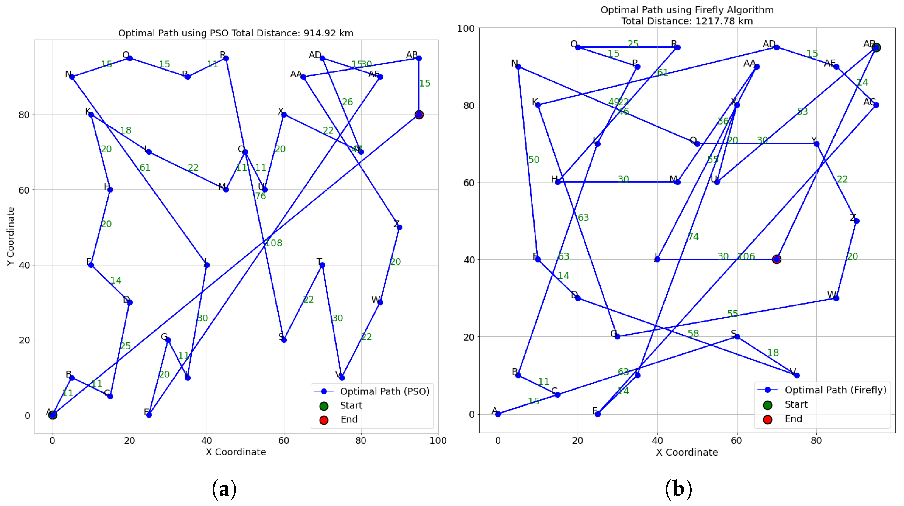
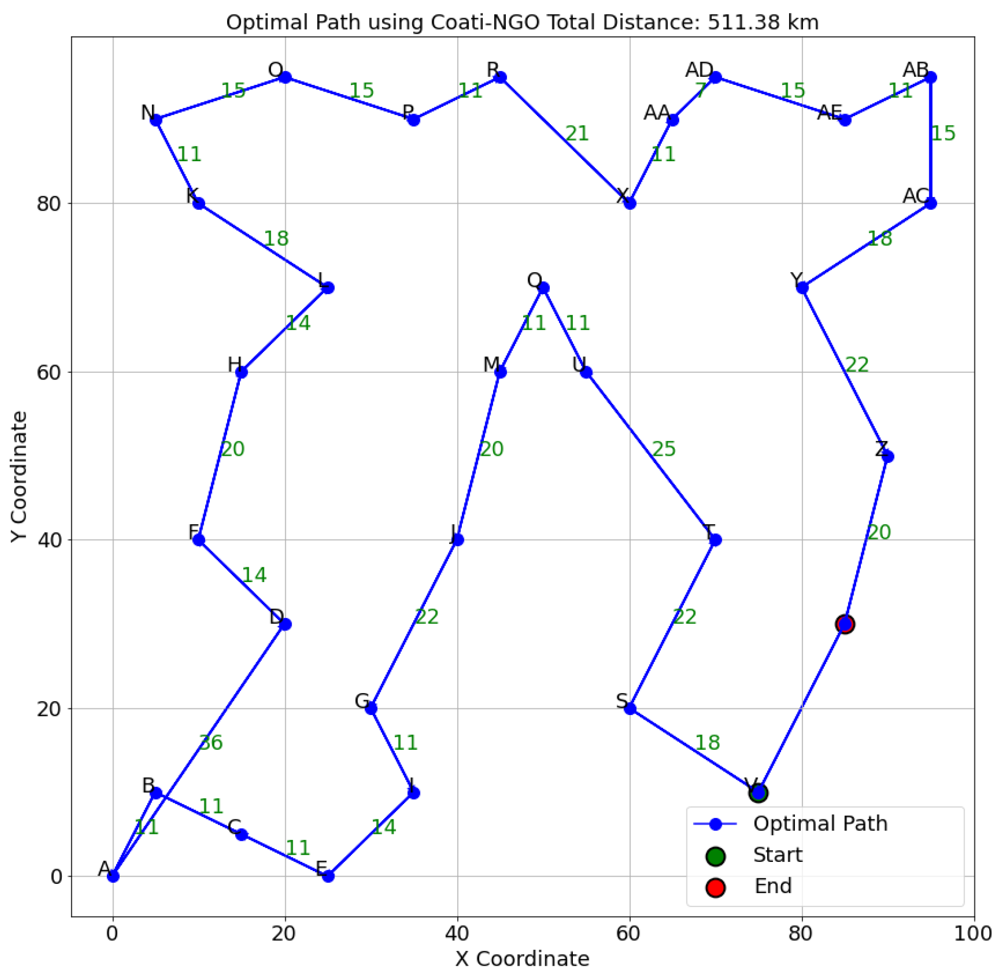
- The Coati–Northern Goshawk Optimization hybrid algorithm reduced fleet travel distances to 511 km, outperforming established optimization techniques.
- Enhanced forecasting and route optimization significantly cut EV fleet energy consumption and costs.
- Real-time IoT data integration supports adaptive, sustainable urban transportation.
Abstract
1. Introduction
2. Related Work
2.1. EV Charging Load Forecasting
2.2. Optimal Pathfinding
2.3. Limitations and Gaps in Existing Research
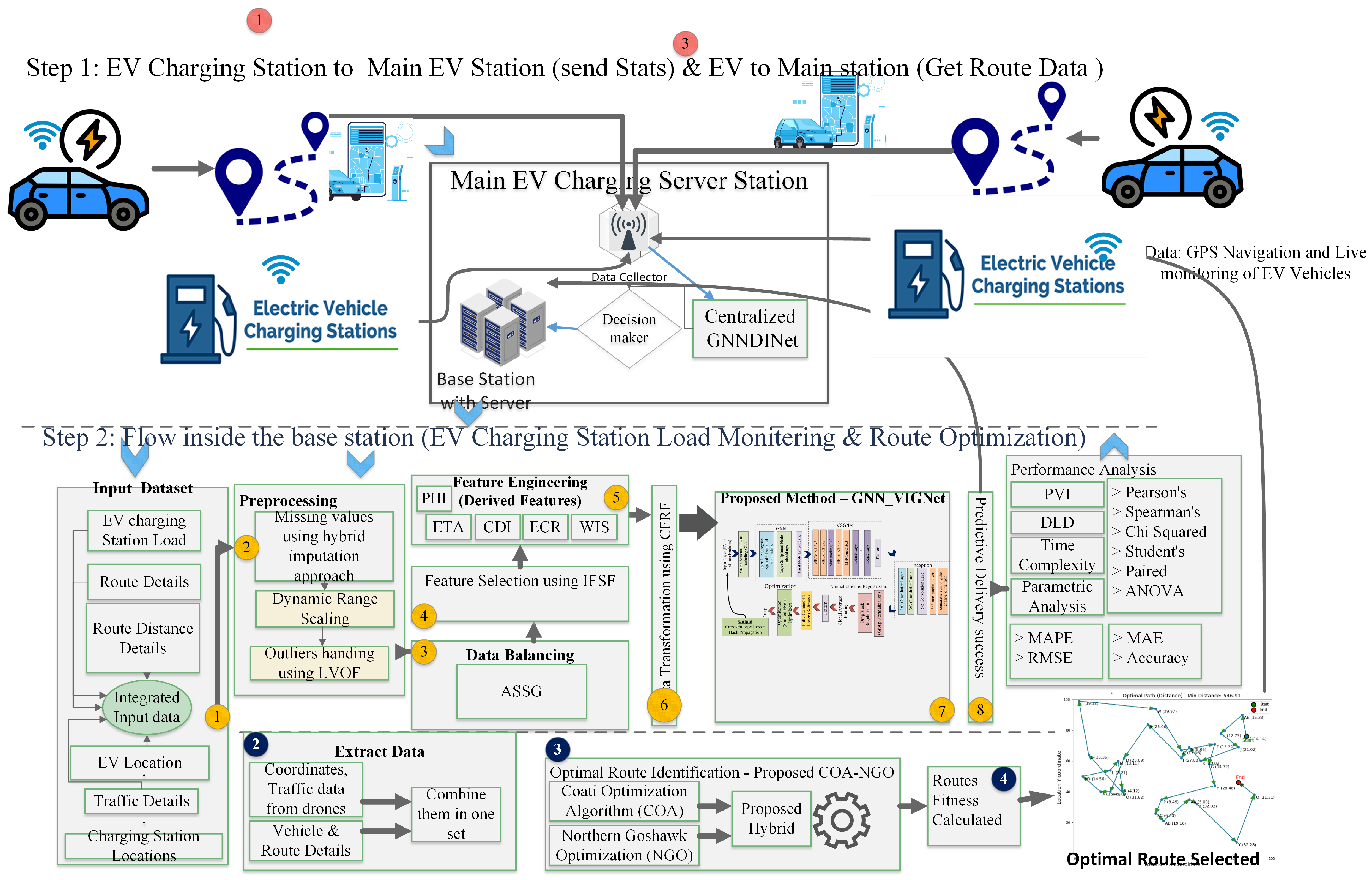
3. Proposed Methodology
3.1. Dataset Description
3.2. Preprocessing Step
3.3. Data Balancing
3.4. Integrated Feature Selection Framework
3.5. Feature Engineering
3.6. Customized Feature Refinement Strategy
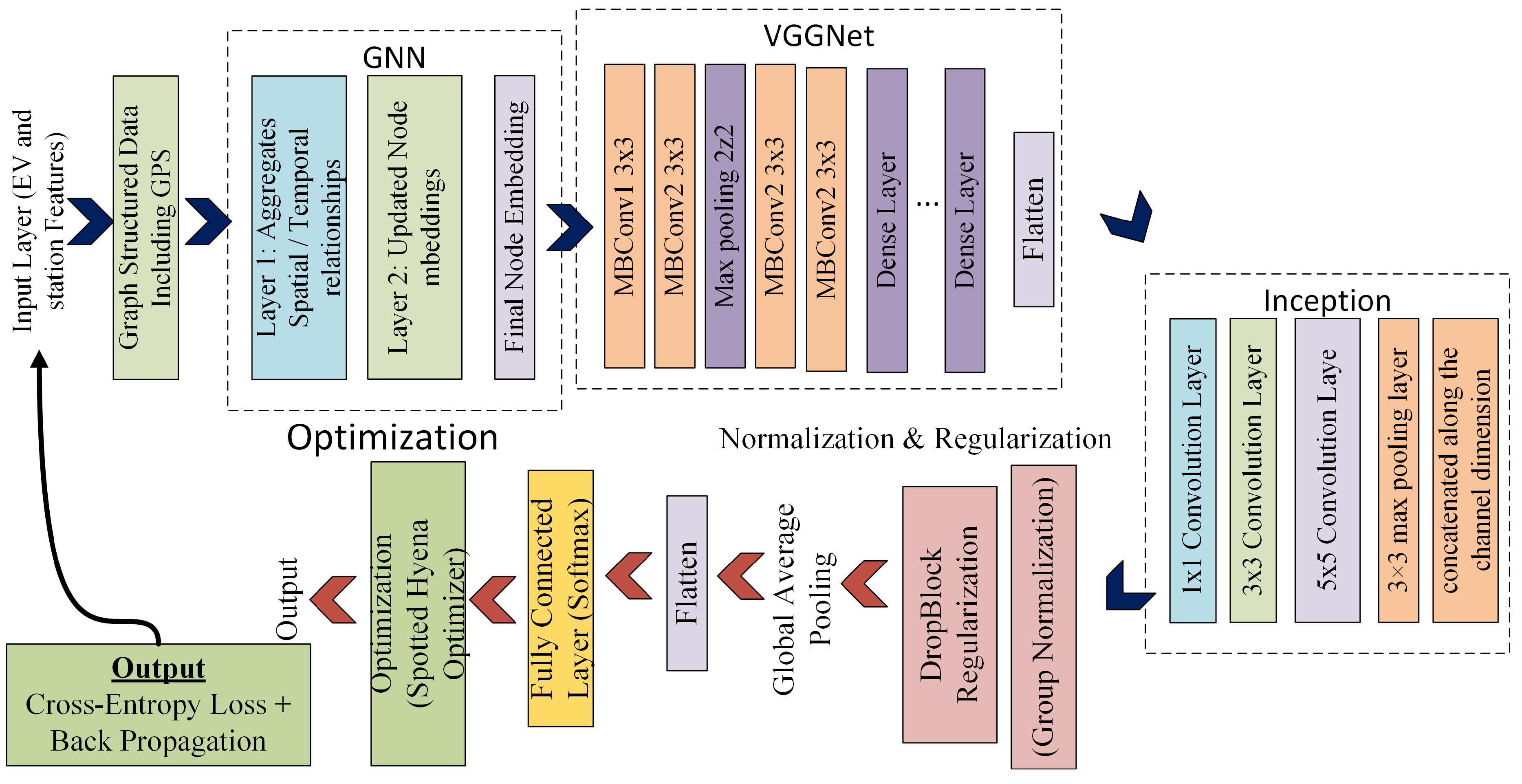
3.7. Forecasting Using GNN-ViGNet
3.8. Hybrid Coati–Northern Goshawk Optimization Algorithm (Coati–NGO) for Route Optimization and Pathfinding
| Algorithm 1 Hybrid Coati–NGO Optimization algorithm for route optimization and pathfinding. |
|
3.9. Evaluation Through Performance Metrics
4. Simulation and Results
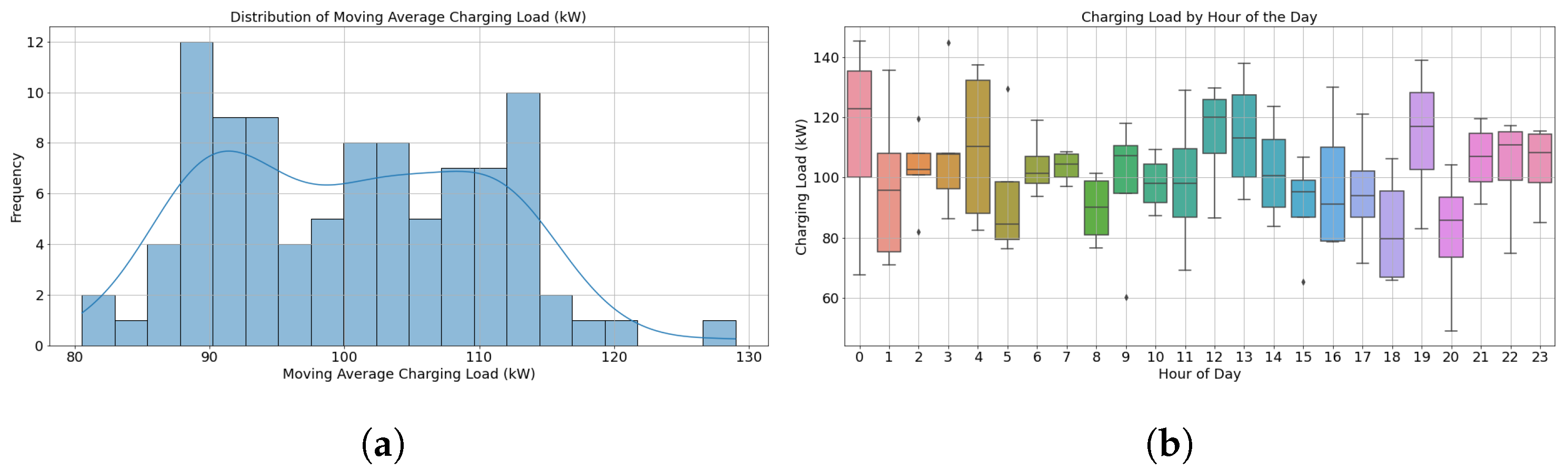
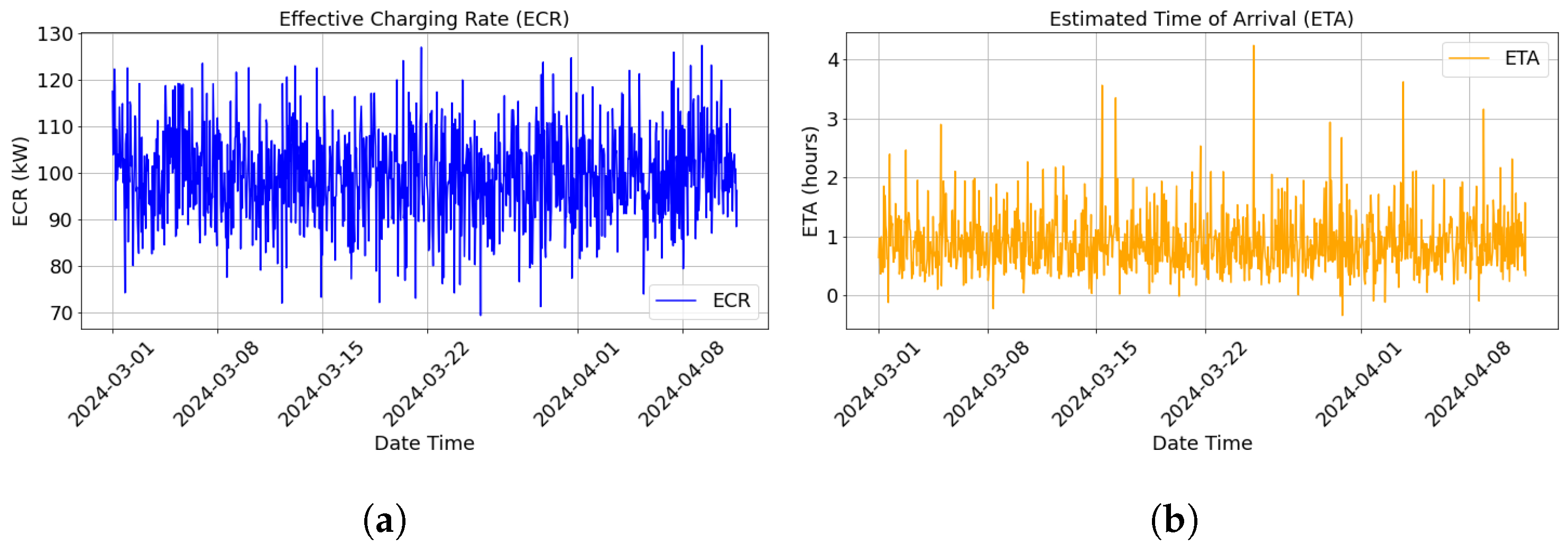
4.1. Charging Load Regression Analysis
4.2. Route Optimization Results
5. Conclusions and Future Work
Funding
Data Availability Statement
Acknowledgments
Conflicts of Interest
Abbreviations
| EVs | Electric vehicles |
| IoT | Internet of Things |
| CPS | Cyber-physical systems |
| HFSHO | Hybrid Firefly–Swarm Hybrid Optimization |
| BCCS | Battery Charging and Switching System |
| BDS | Battery Distribution System |
| DG | Distributed generation |
| GNN | Graph Neural Network |
| CLVI | Charging Load Variance Index |
| FAR | Forecast Accuracy Rate |
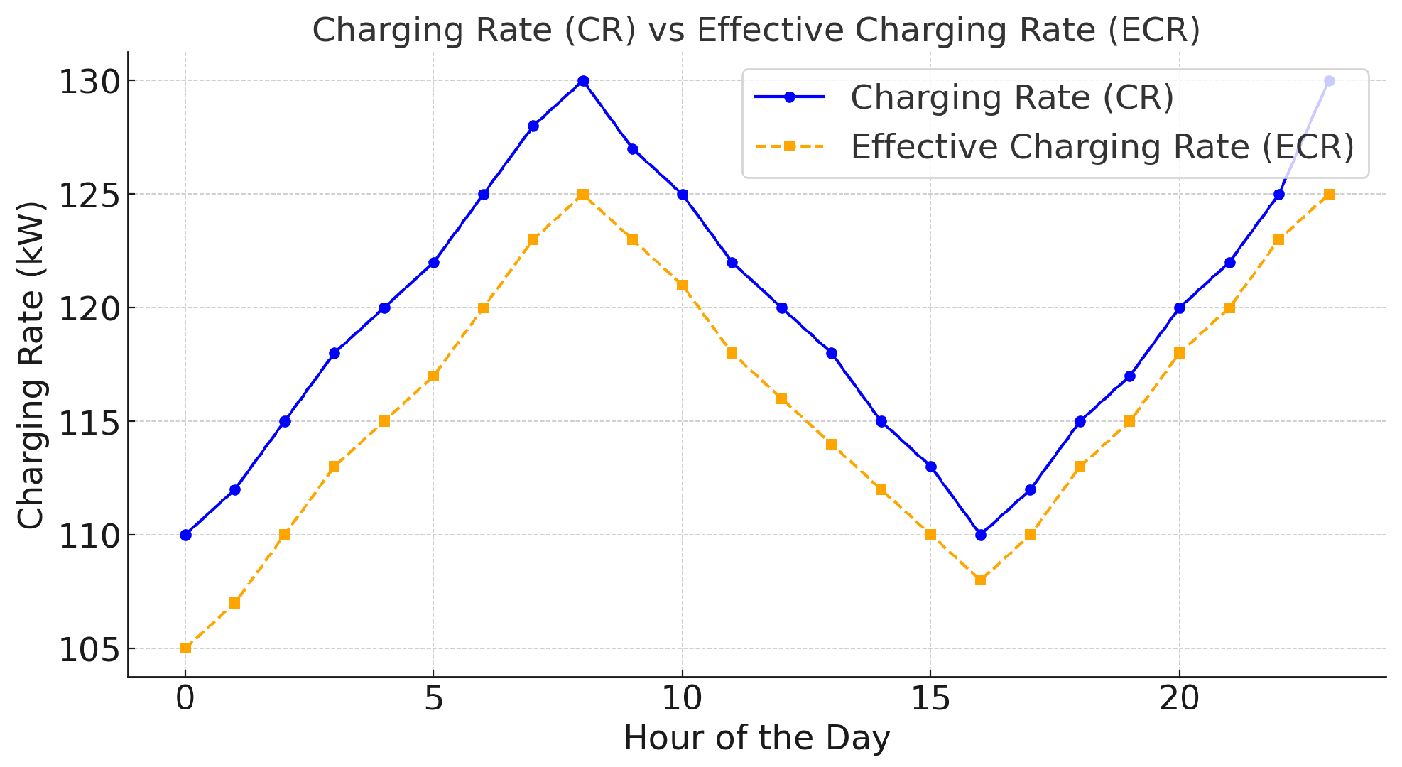
| ECR | Effective Charging Rate |
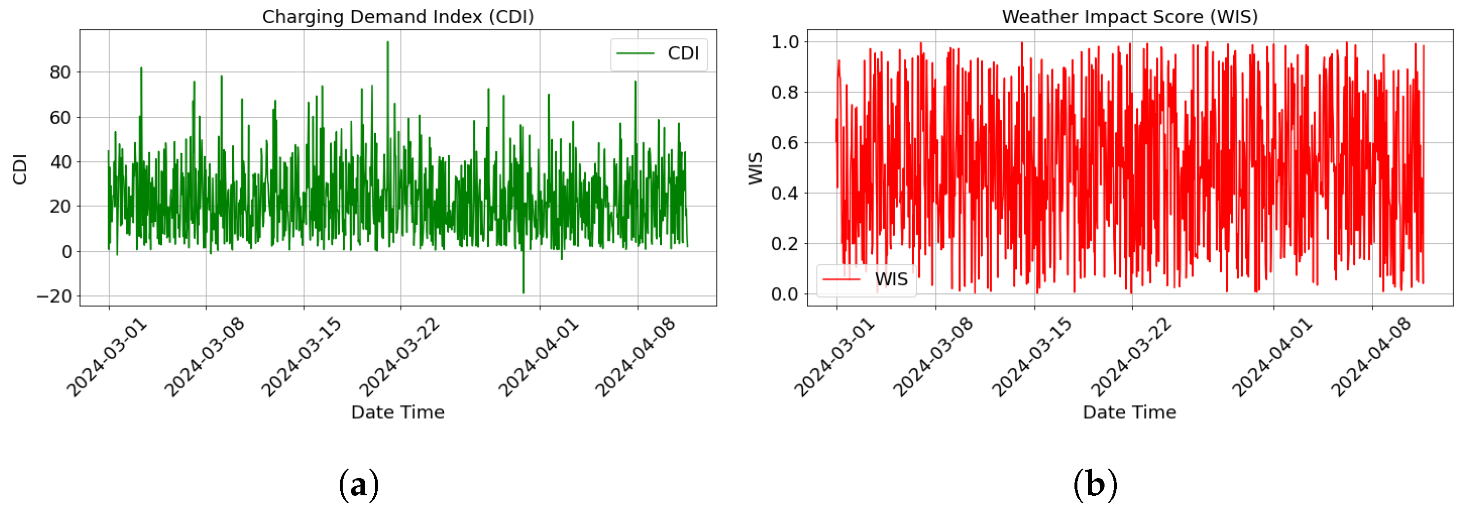
| CDI | Charging Demand Index |
| WIS | Weather Impact Score |
| PHI | Peak Hour Indicator |
| SDRS | Statistical-Driven Rank Selector |
| ASSG | Adaptive Sampling and Synthetic Generation |
| ASO | Adaptive Search Optimization |
| IFSF | Integrated Feature Selection Framework |
| RMSE | Root-Mean-Square Error |
| MAE | Mean Absolute Error |
| DLD | Dynamic Load Deviation |
| PVI | Predictive Variability Index |
| COA | Coati Optimization Algorithm |
| NGO | Northern Goshawk Optimization |
| GPS | Global Positioning System |
| ETA | Estimated Time of Arrival |
| KDE | Kernel density estimate |
References
- Haghani, M.; Sprei, F.; Kazemzadeh, K.; Shahhoseini, Z.; Aghaei, J. Trends in electric vehicles research. J. Appl. Sci. Educ. 2023, 123, 103881. [Google Scholar] [CrossRef]
- Chen, S.; Xiong, J.; Qiu, Y.; Zhao, Y.; Chen, S. A bibliometric analysis of lithium-ion batteries in electric vehicles. J. Energy Storage 2023, 63, 107109. [Google Scholar] [CrossRef]
- Al-Alwash, H.M.; Borcoci, E.; Vochin, M.C.; Balapuwaduge, I.A.; Li, F.Y. Optimization schedule schemes for charging electric vehicles: Overview, challenges, and solutions. IEEE Access 2024, 12, 32801–32818. [Google Scholar] [CrossRef]
- Yuvaraj, T.; Devabalaji, K.R.; Kumar, J.A.; Thanikanti, S.B.; Nwulu, N. A comprehensive review and analysis of the allocation of electric vehicle charging stations in distribution networks. IEEE Access 2024, 12, 5404–5461. [Google Scholar] [CrossRef]
- Aldossary, M.; Alharbi, H.A.; Ayub, N. Optimizing electric vehicle (EV) charging with integrated renewable energy sources: A cloud-based forecasting approach for eco-sustainability. Mathematics 2024, 12, 2627. [Google Scholar] [CrossRef]
- Liu, Y.; Tao, X.; Li, X.; Colombo, A.W.; Hu, S. Artificial intelligence in smart logistics cyber-physical systems: State-of-the-arts and potential applications. IEEE Trans. Ind. Cyber-Phys. Syst. 2023, 1, 1–20. [Google Scholar] [CrossRef]
- Mahyari, E.; Freeman, N.; Yavuz, M. Combining predictive and prescriptive techniques for optimizing electric vehicle fleet charging. Transp. Res. Part C Emerg. Technol. 2023, 152, 104149. [Google Scholar] [CrossRef]
- Zhang, L.; Deng, J.; Li, Q.; Yang, Y.; Lei, M. Research on data center computing resources and energy load co-optimization considering spatial-temporal allocation. Comput. Electr. Eng. 2024, 116, 109206. [Google Scholar] [CrossRef]
- Feng, J.; Chang, X.; Fan, Y.; Luo, W. Electric vehicle charging load prediction model considering traffic conditions and temperature. Processes 2023, 11, 2256. [Google Scholar] [CrossRef]
- Lamontagne, S.; Carvalho, M.; Frejinger, E.; Gendron, B.; Anjos, M.F.; Atallah, R. Optimising electric vehicle charging station placement using advanced discrete choice models. INFORMS J. Comput. 2023, 35, 1195–1213. [Google Scholar] [CrossRef]
- Orzechowski, A.; Lugosch, L.; Shu, H.; Yang, R.; Li, W.; Meyer, B.H. A data-driven framework for medium-term electric vehicle charging demand forecasting. Energy AI 2023, 14, 100267. [Google Scholar] [CrossRef]
- Fresia, M.; Bracco, S. Electric Vehicle Fleet Management for a Prosumer Building with Renewable Generation. Energies 2023, 16, 7213. [Google Scholar] [CrossRef]
- Al-Dahabreh, N.; Sayed, M.A.; Sarieddine, K.; Elhattab, M.; Khabbaz, M.J.; Atallah, R.F.; Assi, C. A data-driven framework for improving public EV charging infrastructure: Modeling and forecasting. IEEE Trans. Intell. Transp. Syst. 2023, 25, 5935–5948. [Google Scholar] [CrossRef]
- Aldossary, M. Multi-Layer Fog-Cloud Architecture for Optimizing the Placement of IoT Applications in Smart Cities. Comput. Mater. Contin. 2023, 75, 633–649. [Google Scholar] [CrossRef]
- Ahmadian, A.; Ghodrati, V.; Gadh, R. Artificial deep neural network enables one-size-fits-all electric vehicle user behavior prediction framework. Appl. Energy 2023, 352, 121884. [Google Scholar] [CrossRef]
- Saxena, A.; Shankar, R.; El-Saadany, E.; Kumar, M.; Al Zaabi, O.; Al Hosani, K.; Muduli, U.R. Intelligent load forecasting and renewable energy integration for enhanced grid reliability. IEEE Trans. Ind. Appl. 2024, 60, 8403–8417. [Google Scholar] [CrossRef]
- Wang, S.; Chen, A.; Wang, P.; Zhuge, C. Predicting electric vehicle charging demand using a heterogeneous spatio-temporal graph convolutional network. Transp. Res. Part C Emerg. Technol. 2023, 153, 104205. [Google Scholar] [CrossRef]
- Milis, G.R.; Gay, C.; Alvarez-Herault, M.C.; Caire, R. Disaggregation model: A novel methodology to estimate customers’ profiles in a low-voltage distribution grid equipped with smart meters. Information 2024, 15, 142. [Google Scholar] [CrossRef]
- He, C.; Zhu, J.; Li, S.; Chen, Z.; Wu, W. Sizing and locating planning of EV centralized-battery-charging-station considering battery logistics system. IEEE Trans. Ind. Appl. 2022, 58, 5184–5197. [Google Scholar] [CrossRef]
- Morais, L.B.S.; Aquila, G.; Faria, V.A.D.; Lima, L.M.M.; Lima, J.W.M.; Queiroz, A.R. Short-term load forecasting using neural networks and global climate models: An application to a large-scale electrical power system. Appl. Energy 2023, 348, 121439. [Google Scholar] [CrossRef]
- Saidani, O.; Alsafyani, M.; Alroobaea, R.; Alturki, N.; Jahangir, R.; Jamel, L. An efficient human activity recognition using hybrid features and transformer model. IEEE Access 2023, 11, 101373. [Google Scholar] [CrossRef]
- Han, D.; Zamee, M.A.; Choi, G.; Kim, T.; Won, D. Optimal electrical vehicle charging planning and routing using real-time trained energy prediction with physics-based powertrain model. IEEE Access 2024, 12, 123250–123266. [Google Scholar] [CrossRef]
- Rashid, M.; Elfouly, T.; Chen, N. A comprehensive survey of electric vehicle charging demand forecasting techniques. IEEE Open J. Veh. Technol. 2024, 5, 1348–1373. [Google Scholar] [CrossRef]
- Daouda, A.S.M.; Atila, Ü. A hybrid particle swarm optimization with tabu search for optimizing aid distribution route. Artif. Intell. Stud. 2024, 7, 10–27. [Google Scholar] [CrossRef]
- Wu, L.; Huang, X.; Cui, J.; Liu, C.; Xiao, W. Modified adaptive ant colony optimization algorithm and its application for solving path planning of mobile robot. Expert Syst. Appl. 2023, 215, 119410. [Google Scholar] [CrossRef]
- Ran, X.; Suyaroj, N.; Tepsan, W.; Ma, J.; Zhou, X.; Deng, W. A hybrid genetic-fuzzy ant colony optimization algorithm for automatic K-means clustering in urban global positioning system. Eng. Appl. Artif. Intell. 2024, 137, 109237. [Google Scholar] [CrossRef]
- Selvarajan, S. A comprehensive study on modern optimization techniques for engineering applications. Artif. Intell. Rev. 2024, 57, 194–217. [Google Scholar] [CrossRef]
- Alqahtani, H.; Kumar, G. Efficient routing strategies for electric and flying vehicles: A comprehensive hybrid metaheuristic review. IEEE Trans. Intell. Veh. 2024. early access. [Google Scholar] [CrossRef]
- Li, X.; Chen, N.; Ma, H.; Nie, F.; Wang, X. A parallel genetic algorithm with variable neighborhood search for the vehicle routing problem in forest fire-fighting. IEEE Trans. Intell. Transp. Syst. 2024, 25, 14359–14375. [Google Scholar] [CrossRef]
- Alshammari, N.F.; Samy, M.M.; Barakat, S. Comprehensive analysis of multi-objective optimization algorithms for sustainable hybrid electric vehicle charging systems. Mathematics 2023, 11, 1741. [Google Scholar] [CrossRef]
- Chauhan, D. Offline learning-based competitive swarm optimizer for non-linear fixed-charge transportation problems. Swarm Evol. Comput. 2024, 88, 101608. [Google Scholar] [CrossRef]
- Younespour, M.; Esmaelian, M.; Kianfar, K. Optimizing the strategic and operational levels of demand-driven MRP using a hybrid GA-PSO algorithm. Comput. Ind. Eng. 2024, 193, 110306. [Google Scholar] [CrossRef]
- John, A. EV charging load dataset and optimal routing [Data set]. Kaggle 2024. [Google Scholar] [CrossRef]
- Dehghani, M.; Montazeri, Z.; Trojovská, E.; Trojovský, P. Coati optimization algorithm: A new bio-inspired metaheuristic algorithm for solving optimization problems. Knowl.-Based Syst. 2023, 259, 110011. [Google Scholar] [CrossRef]
- Dehghani, M.; Hubálovský, Š.; Trojovský, P. Northern goshawk optimization: A new swarm-based algorithm for solving optimization problems. IEEE Access 2021, 9, 162059–162080. [Google Scholar] [CrossRef]
- Aldossary, M.; Alharbi, H.A. An Eco-Friendly Approach for Reducing Carbon Emissions in Cloud Data Centers. Omputers Mater. Contin. 2022, 72, 3175–3193. [Google Scholar] [CrossRef]


| Ref | Technique Used | Objective Achieved | Limitations |
|---|---|---|---|
| [15] | EV load forecasting model using vehicle energy consumption patterns | Captured vehicle energy consumption and driver behavior patterns | Did not incorporate spatiotemporal demand variability |
| [16] | Forecasting model integrating traffic and energy data | Improved load forecast accuracy by considering real-time behaviors | Excluded external factors like weather conditions |
| [17] | Spatial-temporal forecasting approach | Mapped geographical distribution of EV charging demand | Required further testing for scalability |
| [18] | Customer-specific charging profiles for forecasting | Improved forecast accuracy using customer-specific profiles | Did not consider broader impact of distributed generation |
| [19] | Integration of BCCS and BDS in forecasting models | Optimized charging load for large-scale operations | Lacked real-time load adjustments |
| [20] | Monte Carlo simulation for stochastic charging demand modeling | Accounted for random driving behaviors and environmental factors | Substantial computational resources required |
| [21] | Mathematical model for short-term load forecasting | Aggregated load forecasting for electric buses | Focused on buses, limiting general application |
| [22] | Hybrid AI techniques with transformer model | Improved accuracy with AI techniques | Longer training times limited real-time use |
| [23] | Customer preferences and historical data-based forecasting | Forecasted plug-in EV demand based on consumer preferences | Lacked real-time adaptability and short-term adjustments |
| [24] | Tabu Search Algorithm for the Vehicle Routing Problem (VRP) | Efficiently avoided local optima in logistics routing | Did not account for real-time traffic or grid conditions |
| [25] | Modified Ant Colony Optimization (ACO) algorithm | Enhanced global exploration and local optimization | Prone to premature convergence in large-scale operations |
| [26] | Genetic Algorithm (GA) with K-means clustering | Optimized logistics paths but lacked dynamic adjustments | Lacked ability to adjust based on real-time grid conditions |
| [27] | Social Spider Optimization (SSO) algorithm | Optimized logistics routes mimicking spider behavior | No comparative analysis with other algorithms |
| [28] | Gray Wolf Optimizer (GWO) for the VRP | Balanced exploration and exploitation in the VRP | Did not consider EV-specific needs like energy consumption |
| [29] | Enhanced Firefly Algorithm for the VRP with time constraints | Balanced route optimization and time management | Failed to incorporate real-time charging demand |
| [30] | Enhanced Artificial Bee Colony (ABC) algorithm for green logistics | Considered environmental factors in green logistics optimization | Did not optimize charging stops or minimize emissions |
| [31] | Hybrid Particle Swarm Optimization (PSO) algorithm | Balanced constraints like route length and charging needs | Lacked robustness for large-scale fleet management |
| [32] | Hybrid GA with PSO for multiple constraints in logistics | Handled multiple constraints in logistics operations | Did not account for stochastic nature of EV charging needs |
| S.No | Features | Description | S.No | Features | Description |
|---|---|---|---|---|---|
| 1 | Vehicle ID | Unique identifier for each electric vehicle in the dataset. | 15 | Station capacity (EVs) | Maximum number of EVs the charging station can accommodate, categorized. |
| 2 | Battery capacity (kWh) | Total battery capacity of the vehicle, typically around 75 kWh with a normal distribution. | 16 | Time spent charging (mins) | Duration the vehicle spends charging at the station, normally distributed. |
| 3 | State of charge (%) | Percentage indicating the current charge level of the vehicle’s battery. | 17 | Energy drawn (kWh) | Amount of energy drawn during the charging session, following a normal distribution. |
| 4 | Energy consumption rate (kWh/km) | Rate at which the vehicle consumes energy, modeled using an exponential distribution. | 18 | Session start hour | Hour of the day when the charging session starts, represented as an integer (0–23). |
| 5 | Current latitude | Latitude of the vehicle’s current location, centered around Dallas, Texas. | 19 | Fleet size | Total number of vehicles in the fleet, categorized with a bias towards smaller fleets. |
| 6 | Current longitude | Longitude of the vehicle’s current location, centered around Dallas, Texas. | 20 | Fleet schedule | Indicates if the fleet is on time or delayed (0 for on time, 1 for delayed). |
| 7 | Destination latitude | Latitude of the intended destination for the vehicle. | 21 | Temperature (°C) | Current temperature, modeled with a normal distribution around 25 °C. |
| 8 | Destination longitude | Longitude of the intended destination for the vehicle. | 22 | Wind speed (m/s) | Current wind speed, generated using an exponential distribution. |
| 9 | Distance to destination (km) | Estimated distance to the destination, generated using an exponential distribution. | 23 | Precipitation (mm) | Amount of precipitation, following an exponential distribution with most values low. |
| 10 | Traffic data | Count of vehicles on the road, following a Poisson distribution. | 24 | Weekday | Day of the week represented as an integer (0–6), with a skew towards weekdays. |
| 11 | Road conditions | Current state of the road, categorized as ’Good’, ’Average’, or ’Poor’. | 25 | Charging preferences | Indicates charging preferences (0 for no preference, 1 for preference). |
| 12 | Charging station ID | Unique identifier for the charging station, often skewed towards certain IDs. | 26 | Weather conditions | Current weather state categorized as “Clear”, “Cloudy”, “Rain”, or “Storm”. |
| 13 | Charging rate (kW) | Rate at which the charging station delivers power to the vehicle, normally distributed. | 27 | Charging load (kW) | Target label representing the load on the charging station, following a normal distribution. |
| 14 | Queue time (mins) | Estimated wait time at the charging station, following an exponential distribution. |
| Method | R2 | RMSE | DLD | MAPE (%) | Accuracy (%) | PVI | MSE | MAE |
|---|---|---|---|---|---|---|---|---|
| CNN | 0.652 | 0.1175 | 0.0634 | 6.25 | 83.00 | 0.0412 | 0.0138 | 0.0058 |
| GNN-ViGNet (proposed) | 0.982 | 0.0480 | 0.0121 | 1.10 | 98.90 | 0.0089 | 0.0023 | 0.0012 |
| KNN | 0.735 | 0.1220 | 0.0508 | 6.55 | 81.25 | 0.0328 | 0.0149 | 0.0061 |
| ResNet | 0.865 | 0.0959 | 0.0256 | 3.95 | 88.75 | 0.0153 | 0.0092 | 0.0041 |
| DenseNet | 0.871 | 0.0944 | 0.0241 | 3.78 | 88.95 | 0.0149 | 0.0089 | 0.0039 |
| Logistic Regression | 0.685 | 0.1319 | 0.0575 | 7.45 | 77.35 | 0.0385 | 0.0174 | 0.0072 |
| SVM | 0.715 | 0.1253 | 0.0523 | 6.80 | 79.60 | 0.0341 | 0.0157 | 0.0065 |
| EffiResNet | 0.915 | 0.0883 | 0.0194 | 3.20 | 90.00 | 0.0127 | 0.0078 | 0.0034 |
| Method | Total Distance (km) | Iterations to Convergence | Execution Time (s) | Convergence Speed | Exploration | Exploitation |
|---|---|---|---|---|---|---|
| PSO | 919 | 200 | 22 | Moderate | High | Moderate |
| Firefly | 914 | 150 | 18 | Fast | High | High |
| Coati–NGO (proposed) | 511 | 100 | 15 | Very Fast | Balanced | Very High |
| GA | 935 | 250 | 35 | Slow | Moderate | High |
| ACO | 920 | 180 | 25 | Moderate | High | Moderate |
| Simulated Annealing (SA) | 930 | 220 | 28 | Slow | Moderate | Low |
| Tabu Search (TS) | 918 | 190 | 27 | Moderate | Low | High |
| Genetic Algorithm (GA) | 935 | 250 | 30 | Slow | Moderate | High |
| Differential Evolution (DE) | 915 | 160 | 24 | Fast | High | High |
| Hybrid ACO-PSO | 910 | 140 | 20 | Fast | Very High | High |
Disclaimer/Publisher’s Note: The statements, opinions and data contained in all publications are solely those of the individual author(s) and contributor(s) and not of MDPI and/or the editor(s). MDPI and/or the editor(s) disclaim responsibility for any injury to people or property resulting from any ideas, methods, instructions or products referred to in the content. |
© 2024 by the author. Licensee MDPI, Basel, Switzerland. This article is an open access article distributed under the terms and conditions of the Creative Commons Attribution (CC BY) license (https://creativecommons.org/licenses/by/4.0/).
Share and Cite
Aldossary, M. Enhancing Urban Electric Vehicle (EV) Fleet Management Efficiency in Smart Cities: A Predictive Hybrid Deep Learning Framework. Smart Cities 2024, 7, 3678-3704. https://doi.org/10.3390/smartcities7060142
Aldossary M. Enhancing Urban Electric Vehicle (EV) Fleet Management Efficiency in Smart Cities: A Predictive Hybrid Deep Learning Framework. Smart Cities. 2024; 7(6):3678-3704. https://doi.org/10.3390/smartcities7060142
Chicago/Turabian StyleAldossary, Mohammad. 2024. "Enhancing Urban Electric Vehicle (EV) Fleet Management Efficiency in Smart Cities: A Predictive Hybrid Deep Learning Framework" Smart Cities 7, no. 6: 3678-3704. https://doi.org/10.3390/smartcities7060142
APA StyleAldossary, M. (2024). Enhancing Urban Electric Vehicle (EV) Fleet Management Efficiency in Smart Cities: A Predictive Hybrid Deep Learning Framework. Smart Cities, 7(6), 3678-3704. https://doi.org/10.3390/smartcities7060142