Evolutionary Cost Analysis and Computational Intelligence for Energy Efficiency in Internet of Things-Enabled Smart Cities: Multi-Sensor Data Fusion and Resilience to Link and Device Failures

Highlights

What are the main findings?

• Proposed a novel energy-efficient IoT protocol that leverages advanced data fusion grouping, designed to minimize redundant data transmissions and optimize network efficiency.
• Introduced a data fusion sensor head that is selected via a novel MPA fitness function, which is parameterized by key factors such as energy consumption, building occlusions, rotation frequency, proximity to IoT sensors within the data fusion group, and distance to the sink node, while the primary data fusion sensor relay incorporates an innovative relay cost function for enhanced performance.

What is the implication of the main finding?

• Demonstrated superior performance across critical metrics, including network lifespan, energy consumption, throughput, and average delay, surpassing recent approaches in the field.
• Ensured resilience to link and device failures, making the protocol highly suitable for both smart cities and large-scale IoT applications.

Abstract

This work presents an innovative, energy-efficient IoT routing protocol that combines advanced data fusion grouping and routing strategies to effectively tackle the challenges of data management in smart cities. Our protocol employs hierarchical Data Fusion Head (DFH), relay DFHs, and marine predators algorithm, the latter of which is a reliable metaheuristic algorithm which incorporates a fitness function that optimizes parameters such as how closely the Sensor Nodes (SNs) of a data fusion group (DFG) are gathered together, the distance to the sink node, proximity to SNs within the data fusion group, the remaining energy (RE), the Average Scale of Building Occlusions (ASBO), and Primary DFH (PDFH) rotation frequency. A key innovation in our approach is the introduction of data fusion techniques to minimize redundant data transmissions and enhance data quality within DFG. By consolidating data from multiple SNs using fusion algorithms, our protocol reduces the volume of transmitted information, leading to significant energy savings. Our protocol supports both direct routing, where fused data flow straight to the sink node, and multi-hop routing, where a PDF relay is chosen based on an influential relay cost function that considers parameters such as RE, distance to the sink node, and ASBO. Given that the proposed protocol incorporates efficient failure recovery strategies, data redundancy management, and data fusion techniques, it enhances overall system resilience, thereby ensuring high protocol performance even in unforeseen circumstances. Thorough simulations and comparative analysis reveal the protocol’s superior performance across key performance metrics, namely, network lifespan, energy consumption, throughput, and average delay. When compared to the most recent and relevant protocols, including the Particle Swarm Optimization-based energy-efficient clustering protocol (PSO-EEC), linearly decreasing inertia weight PSO (LDIWPSO), Optimized Fuzzy Clustering Algorithm (OFCA), and Novel PSO-based Protocol (NPSOP), our approach achieves very promising results. Specifically, our protocol extends network lifespan by 299% over PSO-EEC, 264% over LDIWPSO, 306% over OFCA, and 249% over NPSOP. It also reduces energy consumption by 254% relative to PSO-EEC, 264% compared to LDIWPSO, 247% against OFCA, and 253% over NPSOP. The throughput improvements reach 67% over PSO-EEC, 59% over LDIWPSO, 53% over OFCA, and 50% over NPSOP. By fusing data and optimizing routing strategies, our protocol sets a new benchmark for energy-efficient IoT DFG, offering a robust solution for diverse IoT deployments.

1. Introduction

The Internet of Things (IoT) has revolutionized various sectors, including automated transportation, smart cities, surveillance systems, healthcare, agriculture, urban security, water management, environmental monitoring, and more, by enabling seamless connectivity and data exchange between a multitude of devices [1,2]. Central to the functioning of IoT ecosystems are Sensor Nodes (SNs), which are responsible for the continuous collection and transmission of data. These SNs, typically deployed in large numbers, form the backbone of IoT networks, making their efficient management and optimization critical to the overall performance and sustainability of these systems [3]. To further enhance the efficiency and functionality of IoT networks, data fusion plays a pivotal role [4]. Data fusion refers to the process of integrating data from multiple SNs to produce more consistent, accurate, and useful information than could be achieved by individual SNs alone [5]. By aggregating and processing data at various levels within the network, such as at individual SNs, clusters, or gateways, data fusion techniques reduce redundancy, mitigate noise, and improve decision-making capabilities [6]. These methods also significantly reduce communication overhead and energy consumption by minimizing the transmission of raw data, thus extending the overall network lifetime. Additionally, data fusion groups (DFGs), where SNs are organized into groups, each managed by a designated leader known as a Data Fusion Head (DFH) and supported by other nodes termed DFG Members (DFGMs), enhance the efficiency of data fusion processes. The hierarchical structure created by data fusion grouping optimizes resource utilization, conserves energy, and extends the network’s lifespan by facilitating localized data aggregation, minimizing redundant data transmission, and balancing the computational and communication load among SNs [7]. Integrating data fusion techniques within clustered IoT architectures ensures scalable, energy-efficient, and robust operations, which are essential for the continued evolution of IoT applications across diverse domains [8,9].

1.1. Problem Statement and Motivation

The management of vast IoT sensor networks poses significant challenges, particularly in terms of energy efficiency, data transmission reliability, and network longevity. One critical issue is the selection of DFHs, which are pivotal in clustering operations [10]. DFHs are responsible for aggregating data from their respective DFGMs, performing data processing, and transmitting the aggregated data to the sink node or other relay DFHs. However, the role of DFHs is energy-intensive, and inefficient DFHs selection can lead to the rapid depletion of energy resources, uneven load distribution, and shortened network lifespan [11]. Consequently, optimal DFH selection is vital for the success of clustering strategies [12]. Another key challenge is defining the optimal number of DFGs and achieving an even distribution of SNs within groups. IoT networks often operate in dynamic environments where network topology and conditions can change rapidly, making traditional DFH selection methods, often reliant solely on remaining energy (RE), inadequate. These conventional approaches struggle to adapt to IoT’s dynamic nature, resulting in energy imbalances and premature node failures [13]. Emerging technologies like machine learning offer promising solutions by introducing adaptability and context-awareness to DFH selection, addressing these limitations effectively [14,15]. Furthermore, optimization within DFGs remains critical since SNs typically rely on limited power sources such as batteries, and frequent recharging or replacement is often infeasible [16]. Optimizing energy consumption while ensuring reliable data transmission and minimal latency is essential, especially for real-time applications such as healthcare monitoring, where timely and accurate data are critical. The dynamic nature of IoT networks demands that algorithms adapt to changes in topology, balance the load among SNs, and efficiently manage limited computational and storage resources. Data fusion presents another significant challenge in IoT networks. The process of aggregating and synthesizing data from multiple SNs to produce meaningful and accurate outputs is computationally intensive and often constrained by limited resources [17]. Inefficient data fusion mechanisms can result in redundant transmissions, increased energy consumption, and higher latency. Additionally, ensuring the quality of fused data is critical for applications such as environmental monitoring and industrial automation, where decisions depend on accurate, real-time information. Despite the availability of sophisticated data fusion techniques, their integration into resource-constrained IoT networks poses challenges related to scalability, adaptability, and energy efficiency [18]. The integration of emerging technologies such as machine learning and Artificial Intelligence (AI), particularly Computational Intelligence (CI), into DFH selection, data fusion grouping, and data fusion offers both opportunities and challenges [19]. Optimization methods such as Genetic Algorithms (GA) [20], Particle Swarm Optimization (PSO) [21], and Ant Colony Optimization (ACO) [22] have demonstrated significant potential in enabling context-aware decision-making by considering multiple criteria, including RE, node connectivity, communication overhead, and data redundancy [23]. These methods can significantly enhance clustering and data fusion efficiency, resulting in balanced energy consumption, reduced data redundancy, and enhanced network longevity [24]. However, choosing the appropriate optimization technique requires a careful consideration of network characteristics, such as node mobility, density, heterogeneity, and resource constraints, underscoring the need for lightweight, adaptive, and real-time algorithms tailored for specific IoT deployment scenarios [25]. Routing is equally critical, as it manages the pathways for data packets traveling from SNs to the sink node or relay DFHs. Effective routing protocols ensure reliable data transmission, minimize energy consumption, and balance the load among DFHs [26,27]. Conversely, inefficient routing can lead to imbalanced load distribution, increased latency, and excessive energy consumption. Adaptive routing protocols that consider factors such as SN distance to the sink node, RE levels, and data aggregation potential are essential for maintaining network performance under varying conditions [28]. To this end, efficient DFH selection, data fusion grouping optimization, and adaptive routing are foundational to addressing the challenges of IoT networks. Achieving energy-efficient, reliable, and scalable solutions is paramount for enabling IoT’s full potential across diverse applications, from smart cities to industrial automation and healthcare monitoring. However, these problems are intertwined and demand holistic solutions that integrate data fusion grouping and routing optimization. Emerging machine learning and AI-driven techniques offer the potential to address these challenges, but their application to resource-constrained, dynamic IoT environments requires further exploration. This paper aims to address these challenges by exploring state-of-the-art techniques for DFH selection, data fusion grouping optimization, data fusion, and adaptive routing. By integrating emerging optimization methods and evaluating their effectiveness in real-world scenarios, the study seeks to contribute to the development of efficient, scalable, and adaptive solutions for IoT networks, unlocking their full potential across various domains.

1.2. Research Gaps, Our Methodology, and Contributions

In the realm of IoT networks, significant research gaps persist in the areas of clustering, optimization methods, and data fusion for DFH selection and routing. Current clustering and data fusion techniques often struggle with scalability and adaptability to dynamic network conditions, leading to inefficient resource utilization and reduced network lifespan. Moreover, optimization methods for DFH selection require further refinement to effectively balance energy consumption, ensure load distribution, and maintain robust communication links. Existing algorithms frequently overlook heterogeneous network environments, where SNs may have varying energy levels and capabilities. Additionally, routing protocols face challenges in handling the diverse and fluctuating data traffic typical in IoT applications. Many protocols lack the ability to dynamically adjust routes in real-time, resulting in increased latency and energy expenditure. Addressing these gaps necessitates the development of more advanced, adaptable algorithms that can optimize performance across varied IoT network scenarios, ensuring reliability, energy efficiency, and prolonged operational life. Essentially, there is an interest in utilizing CI and data fusion for routing protocols in IoT applications. These applications require simple, stable, and reasonably priced networking solutions. In addition, improving network performance presents a complex optimization problem. In response to the aforementioned challenges, bioinspired evolutionary approaches like PSO [29] and ACO [22] have gained importance in determining the optimal paths for the routing protocols. These optimization techniques compute the Data Fusion Fitness Function (DFFF) iteratively throughout a population and compare every solution to the best one in order to identify the optimum routing option. Indeed, DFFF definitions have a major influence on selecting optimal DFHs. In the existing literature, DFFFs have frequently been designed with uniform or arbitrary weight values, regardless of the location of SNs or their RE. Furthermore, selecting the optimization approach is seen to be a difficult task. It is important to note that network performance concerns are exacerbated by the expanding size of the network and the number of SNs. IoT researchers have responded to this by proposing energy-efficient routing protocols that might allow networks to function for extended periods of time without requiring battery replacements or recharges, especially in harsh environments. As a result, the primary objective of this work is to put forward a practical routing protocol that will improve network performance and cure previous issues. Only a limited number of metaheuristic algorithms have gained broad traction in general. This is mainly because of its energy-inefficient and computationally intensive features, which are unable to ensure that there is enough RE to increase network lifespan. Therefore, this is why the most appropriate metaheuristic algorithm must be chosen.

Importantly, this work tackles the faults of currently available clustering and data fusion algorithms while likewise utilizing a superior metaheuristic algorithm, named the Marine Predators Algorithm (MPA) for Primary DFH (PDFH) selection in this particular context, to overcome energy efficiency considerations [30]. Under the proposed protocol, the network lifespan is distributed evenly among rounds. In fact, the setup and steady state phases are covered in the first round, and only the steady state phase is addressed in the following rounds for data fusion and transmission purposes. On the other hand, the setup step could be carried out during regrouping (PDFH reselection). The unique feature of this protocol is that SNs are able to perceive and send information over the duration of the Round Time (RT) to handle data fusion in a professional manner. Additionally, a set of SNs is randomly distributed inside a rectangle network sensory geographical area. The sink node broadcasts a request information message to every SN in the network. Firstly, the sink node only completes the setup phase once in an effort to minimize the number of control messages generated during DFG establishment. In response, the SNs reply with an SN’s information message, which contains the SN’s location and its energy. Consequently, the sink node divides the sensing area into hexagonal DFGs of equal size. This division is based on data received from each SN. Subsequently, the sink node determines a PDFH for every cluster. In essence, the innovative proposed protocol, presented in this paper, employs a data fusion strategy in which each group’s best PDFH is selected using the MPA, which has clearly become more popular in the last several years, as seen by the 2029 total citations it received according to a Google Scholar survey that was conducted up to February 8, 2025. The novel aspect of the proposed protocol is figuring out the DFFF, which takes into account not only necessary parameters, such as the average distance between DFGMs, DFGMs’ RE, their distance from the sink node, Average Scale of Building Occlusions (ASBO), and PDFH rotation times, but also a weight assigned to each parameter, which is determined by a trial-and-error procedure following the execution of a colossal number of assessments and the selection of values that provide the best possible outcomes for the performance of the network. Intriguingly, in order to receive optimal PDFH, this DFFF is considered to be the objective function of the MPA that has to be minimized. In other words, the DFFF with the lowest values of the aforementioned parameters is the best one. In addition to the PDFH selection, our proposed protocol is batch-based. This means the regrouping (PDFHs reselection) does not occur every round but after a batch of rounds. In order to achieve this, the RE of the selected PDFH is compared with the average RE of DFGMs (energy threshold); if the RE of PDFH falls under the threshold, regrouping (PDFH reselection) is carried out by sending a disjoin message by a PDFH to the sink node and all SNs in the networks as an indication to start the process of regrouping. For data fusion and transmission, the proposed protocol without routing is suggested in order to send data from SNs to their PDFH, and then the PDFHs aggregate the data and then send them directly to the sink node (i.e., single hop communication) by assigning a Time Slot (TS) for each SN based on a novel Time Division Multiple Access (TDMA) technique. On the other hand, the proposed protocol with multi-hop routing transmits the data from SNs to their PDFHs, and then the PDFHs gather the data and then send them directly to the sink node (i.e., single hop communication) if the distance between PDFH and the sink node is less than the crossover distance (87 m). Otherwise, the protocol utilizes a cutting-edge Relay Data Fusion Cost Function (RDFCF) to identify PRs to route the data until reaching the sink node (i.e., multi-hop communication). The distance between the PDFH and the list of PDFHs in the upper layers, their respective RE, and ASBO are the three influential factors used to create the RDFCF. Since a PDFH with the lowest RDFCF is selected as the next relay PDFH, the RDFCF should be reduced. The notion of relay PDFHs and RDFCF reduces control overhead and the distance between PDFHs and the sink node, and intelligently relieves congestion at PDFHs near the sink node by distributing the load between PDFHs. By using such an approach, SNs that are located far away from the sink node are guaranteed to preserve energy. In general, all of the techniques mentioned are liable for saving energy and effectively increasing the network’s lifespan.

Impressively, as per the best of our knowledge, there is no paper in the field highlighting and covering the innovative aspects of our paper so far, particularly integrating data fusion techniques within clustered IoT architectures, making it distinguishable among others. In light of this, the major contributions of this paper are delineated as follows:

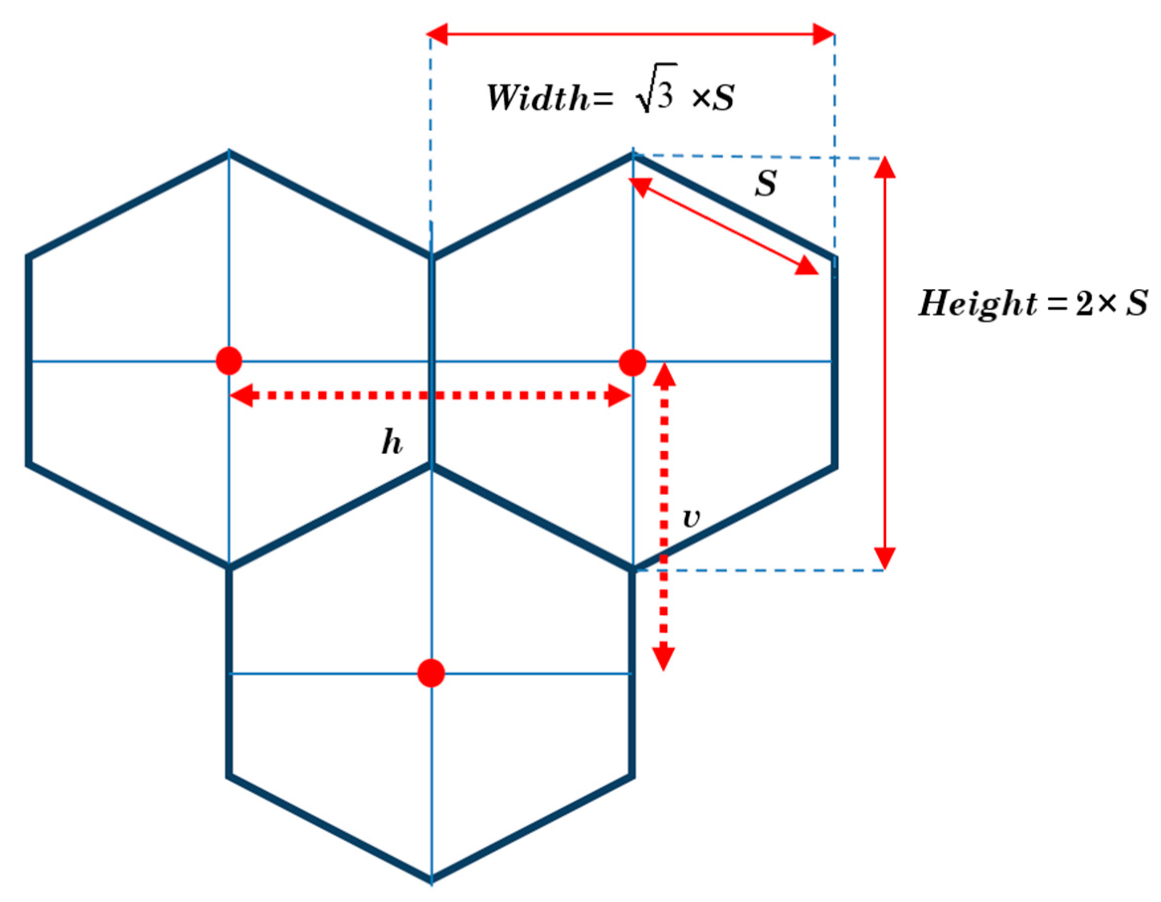
• The introduction of a pioneering adaptive and dynamic DFG division methodology based on a hexagonal structure. The division process dynamically adjusts in response to the presence and distribution of SNs within the network vicinity. This approach ensures optimal coverage, balanced node participation, and efficient scalability, aligning the DFGs framework with the growth and distribution patterns of IoT SNs.
• The proposal of a high-efficiency DFG mechanism that continuously adapts to varying network densities. The groups dynamically evolve in response to real-time network conditions, optimizing resource utilization and balancing workloads. This adaptive framework enhances the responsiveness of the network while maintaining low latency and robust operational efficiency.
• For DFGs, there is an implementation of an innovative method for selecting the optimal PDFH, First Secondary DFH (FSDFH), and Second SDFH (SSDFH) for each DFG utilizing the MPA. This approach incorporates highly effective and complex criteria for DFFF, such as the SNs’ distance from the sink node, their RE, and the average distance between DFGMs, ASBO, and PDFH rotation times, effectively preserving SNs’ energy and prolonging the network’s lifespan.
• The implementation of a novel parameter, namely ASBO, where, to the best of our knowledge, we are the first researchers who have introduced and implemented this factor in-depth in the DFFF and RDFCF. The exact definition of ASBO is demonstrated in Section 5.2.2.
• For relaying, the proposed protocol utilizes innovative RDFCF to select a Primary Data Fusion Relay (PDFR), First Secondary DFR (FSDFR), and Second SDFR (SSDFR) based on the candidate PDFR’s RE, its distance from the sink node, PDFH, and ASBO in order to select optimal PDFRs, particularly those situated at significant distances from the sink node, thereby conserving PDFHs’ energy with demonstrated efficiency.
• The optimization and management of resource utilization and data redundancy reduction by applying data fusion techniques for device/link failures and recovery, data redundancy, and building occlusion. In particular, we analyze the issue of data redundancy among relatively close SNs, and in light of this, we provide an efficient data fusion management approach that guarantees a coherent and efficient protocol. Specialist recovery techniques are also employed to address device and link failures, consolidating the protocol and enhancing its overall performance. We also examine the effects of building occlusions at various elevations and appropriate mitigation strategies.
• The illustration of the PDFH, FSDFH, and SSDFH selection processes employing MPA within the proposed protocol through a detailed and comprehensible example, enhancing readers’ understanding and proficiency in this aspect.
• The comprehensive performance evaluation of the proposed protocol through an extensive series of simulations, considering key network performance evaluation metrics including network lifespan, energy consumption, throughput, and average delay. Comprehensive comparisons with existing protocols demonstrate the effectiveness of the proposed protocol without and with multi-hop routing.

This paper is organized as follows: Section 2 offers a thorough discussion of previous related works, focusing on the design of energy-efficient routing protocols, especially for the election of PDFH, as well as optimization methods. In Section 3, we provide a comprehensive overview of the MPA and its applications. The system model is demonstrated in Section 4, while Section 5 is dedicated to the proposed protocol, presenting a detailed demonstration of it. Section 6 meticulously displays and analyzes the simulation results. Finally, Section 7 concludes the paper and offers key recommendations.

2. Related Works

A review of the pertinent literature can be found in this section. In the last twenty years, the adoption of the IoT has received close attention from academics across diverse disciplines, influencing various facets of daily life. The essence of IoT lies in establishing connectivity among all entities, enabling human interaction with objects through a variety of SNs. In IoT, where battery-powered SNs are often deployed in remote or inaccessible areas, adopting energy-efficient strategies becomes paramount since these SNs have finite energy sources. To mitigate this challenge, energy consumption must be minimized. Numerous approaches have been proposed to prolong the lifespan of the IoT and enhance overall network longevity. The Cluster Head (CH) selection emerges as a crucial technique to ensure network stability by organizing SNs into clusters within the network area via machine learning, and CHs are selected from these clusters according to predetermined criteria. The utilization of CI, which is becoming more and more common in WSNs, the IoT, and crowd-sensing applications, can help to achieve this [31]. Numerous studies have explored metaheuristic optimization algorithm-based clustering techniques to address the ambiguity in WSNs. While various CH selection methods have been introduced, optimizing energy efficiency remains a persistent challenge in the IoT.

Energy and Distance-Based CH Selection (EDB-CHS) and EDB-CHS with Balanced Objective Function (EDB-CHS-BOF) are two innovative protocols for CH selection that were proposed by Darabkh et al. [32]. The objectives of these protocols are to prevent premature SN breakdown, handle imbalances in energy consumption among SNs, and increase the lifespan of the network as a whole. They suggest a hexagonal cluster structure for the EDB-CHS protocol and generate an expression with a closed form to find the ideal number of CHs in the network. They further offer an effective approach for choosing a CH based on a threshold probability that bears in mind many aspects, such as SN’s probability of becoming a CH, closeness to the sink node, and SN’s RE. On the other hand, long-distance communications between adjacent CHs are the focus of the EDB-CHS-BOF protocol. A new threshold probability for each SN to become a CH in a given round is proposed in this protocol. To guarantee a uniform distribution of CHs over the network, a balanced objective function is also introduced. Most importantly, the findings from experiments show that these proposed protocols perform better, far exceeding their rivals, especially when it comes to throughput and network longevity. The author in [33] utilizes two metaheuristic algorithms for clustering and routing tasks. Firstly, they employ the Whale Optimization Algorithm (WOA) to cluster the network, forming optimal CHs through a method called WOA-clustering. Subsequently, for routing these CHs to the sink node, they utilize the Harris Hawks Optimization (HHO) algorithm in a routing method termed HHO-Routing. By adopting these approaches, they achieve reduced energy consumption for data transmission to the sink node. To validate the efficacy of the proposed protocol, comparisons with existing algorithms are conducted for a more comprehensive assessment. The simulation outcomes reveal enhancements in data transmission rates, energy consumption, and the number of rounds before the first node dies.

Motivated by the need to enhance energy efficiency in underwater WSNs and extend network lifespan, the authors in [34] presented an energy-efficient clustering and multi-hop routing protocol employing metaheuristic-based algorithms. However, current metaheuristic-based techniques often employ distinct algorithms for clustering and multi-hop routing, resulting in increased computational intricacy, diverse initialization procedures, and challenges in hyperparameter tuning. To address these limitations, a novel hierarchical structure named the Hierarchical Chimp Optimization Algorithm (HChOA) for both clustering and multi-hop routing tasks is introduced. The proposed HChOA is evaluated using various metrics through extensive simulations, comparing its performance with different protocols. The results demonstrate that HChOA outperforms others concerning network lifespan and energy consumption. In essence, Darabkh et al. [35] presented new strategies that improve energy consumption in the network as a whole, even when several important network factors are considered. The network is divided equitably into several clusters by the clustering process, and each cluster elects a CH using PSO, taking into account crucial factors such as SN’s RE and distance from the Mobile Sink (MS). Moreover, in the proposed protocol, the movement of the MS is coordinated to distribute energy consumption evenly across all SNs. This is achieved by implementing a circular trajectory with a dynamic radius and constant angular velocity. The MS initiates its movement from the center of the network, traversing along the radius in both forward and reverse directions. This strategic movement pattern ensures that SNs in closer proximity to the sink consume less energy compared to those located farther away, thus enhancing the network’s energy efficiency and overall performance. Additionally, the MS broadcasts its initial position, enabling each SN to predict the sink’s instantaneous position. Furthermore, the clustering overhead is significantly minimized as the setup phase is infrequently invoked. To evaluate the performance of the proposed protocol regarding network lifetime and overall power consumption across arbitrary rounds, extensive simulations have been conducted, demonstrating conclusively that the innovations embedded in this protocol significantly surpass those of its counterparts. The authors in [36] have introduced a novel optimization algorithm called SWARAM (Osprey Optimization Algorithm-based Energy-Efficient CH Selection) for WSNs in the context of the IoT to optimize CH selection. The SWARAM approach comprises two phases: cluster construction and CH selection, where SNs are first clustered based on Euclidean distance, followed by CH selection using the SWARAM technique. The performance results of SWARAM are compared with existing CH selection and demonstrate that SWARAM enhances packet delivery ratio and network lifetime by 10% each, thereby improving the overall network performance. Ensemble clustering has long demonstrated its prowess in unsupervised learning, but traditional Co-Association (CA) matrix-based methods still fall short in several critical areas. These methods tend to focus solely on strengthening pairwise CA within the same cluster, often neglecting the valuable inter-cluster relationships that provide a more comprehensive understanding of the data. Additionally, they rely heavily on external clustering methods such as spectral clustering to derive results from the CA matrix, and they fail to adaptively assign weights to individual base clustering results, treating all contributions as equally important regardless of their relevance or quality. To address these limitations, the authors in [37] proposed WEC-FCA, a novel Weighted adaptive Ensemble Clustering method powered by a Fuzzy CA (FCA) matrix. The FCA matrix revolutionizes ensemble clustering by capturing both CA and inter-cluster relationships, offering a more nuanced representation of the dataset. By incorporating a rank constraint into the FCA matrix, they designed an innovative optimization framework that directly outputs the optimal ensemble FCA matrix, inherently aligned with the true number of clusters and eliminating the need for external clustering methods. Furthermore, WEC-FCA dynamically assigns weights to each base clustering result using Shannon entropy, ensuring that the most significant contributions are emphasized during the optimization process. The experimental results on both synthetic and real-world datasets demonstrate the superiority of WEC-FCA, consistently achieving comparable or better clustering performance than state-of-the-art methods, all while addressing the fundamental shortcomings of traditional approaches. The rapid development of advanced communication technologies has positioned location information as a cornerstone for enabling context-aware and location-aware intelligent services. Among these, modern Intelligent Transportation Systems (ITS) present the most stringent demands for real-time, highly accurate, and privacy-preserving location data. To address these challenges, the authors in [38] introduced a novel Spatial–Temporal Federated Transfer Learning (ST-FTL) framework, which combines multi-sensor data fusion with advanced privacy-preserving techniques to enhance cooperative positioning in urban ITS. The framework employs a three-layer architecture that integrates Federated Learning (FL) with Transfer Learning (TL), enabling a faster convergence of the global model, reduced communication costs, and improved prediction accuracy, even in scenarios with limited local data, such as urban canyons. A density-based spatial–temporal clustering algorithm is developed to identify optimal source domains for transfer, ensuring similarity between regions and improving cross-region model performance. Additionally, a convolutional-gated unit is proposed to filter irrelevant features and generate meaningful new features, enhancing global model initialization and weight aggregation. Locally, a multi-sensor data fusion model combines GPS and inertial measurement unit data through an improved time-aware asymmetric attention mechanism, which dynamically adjusts the importance of each data source based on contextual relevance. Furthermore, a streamlined Siamese network structure enables lightweight data augmentation by leveraging historical data from individual vehicles, addressing the challenge of insufficient training data. Experimental evaluations using two public datasets demonstrate the superiority of the proposed ST-FTL framework over state-of-the-art methods, achieving enhanced positioning accuracy, faster convergence, and robust performance in urban ITS scenarios.

The references [39,40,41,42] cite works that are extremely pertinent to our suggested protocol. In [39], a PSO-based energy-efficient clustering protocol (PSO-EEC) is introduced with the purpose of improving network lifespan. This protocol utilizes the PSO algorithm to select CHs and relay SNs within the network. CHs are chosen based on an FF derived from the PSO algorithm, which takes into account the SN energy ratio (initial and RE), distance from SNs to CHs, and SN degree to determine the most suitable SN for the CH role. For data transmission to the sink node, PSO-EEC employs a fitness value based on the RE of CHs and distance to the sink node to select relay SNs for multi-hop data transfer. The simulation results demonstrate that the proposed protocol outperforms existing techniques in terms of performance parameters, including energy consumption, network lifetime, and throughput. To develop effective clusters, a linearly decreasing inertia weight PSO-based Clustering technique (LDIWPSOC) is presented in [40]. In LDIWPSOC, PSO initially employs a particle encoding mechanism to indicate the indices of SNs selected as CHs by representing particles using SN coordinates. Coordinates and velocity are generated at random during particle initialization. Subsequently, in order to find the global and personal optimum solutions, an FF is derived considering parameters such as the intra-cluster distance, the distance between CHs and the sink node, and the RE of selected CHs. Finally, in order to update the position and velocity of the particles, a linearly decreasing inertia weight has been provided, where personal and global best solutions are iteratively updated until the global best solution is achieved. This stimulates exploration at the start of the iteration and exploitation as it becomes closer to the end. In this way, it is feasible to significantly increase search accuracy and quickly find the global optimal solution without settling for the local optima. SNs with significant disparities in their neighbors might be chosen as CHs, resulting in excessive intra-cluster energy consumption. An Optimized Fuzzy Clustering Algorithm (OFCA) is proposed in [41] for the selection of CHs and a routing protocol for data transmission to the sink node. In the OFCA, CHs are chosen based on distance from the sink node, RE, and SN concentration using type-1 fuzzy logic system. To establish an energy-efficient routing path to the sink node, other CHs are utilized via PSO. The FF of PSO is designed to determine the local and global best of particles, thereby increasing the network lifespan. As in standard PSO, the global best solution is determined by first initializing the particles and then updating them until a particle with an optimal fitness value represents the global best solution. As a result, CHs that have higher concentration, a less than average distance to the sink node, and higher levels of RE are selected as relay SNs. The PSO-based routing scheme in OFCA selects optimal CHs to establish efficient routing paths for data forwarding, thereby minimizing the energy consumption of CHs involved in inter-cluster communication and enhancing network lifetime. However, employing a single path from the source node to the destination may not guarantee high Quality of Service (QoS) for the network. The simulation results demonstrate that OFCA achieves a longer network lifespan and facilitates the transmission of more messages to the sink node. The authors in [42] introduced a novel clustering and routing protocol named NPSOP, based on PSO, aimed at extending network lifespan while ensuring energy efficiency and load balance. NPSOP employs PSO to select CHs and determine routes for each CH simultaneously, with particle components constrained by RMs such as distance to the sink node, RE, and centrality to enhance convergence speed. An FF, considering both network load balancing and energy consumption, evaluates particle quality. Additionally, an adaptive inertial weight is utilized to update particle status, preventing trapping in local optima and facilitating convergence to the global optimal solution iteratively. Extensive experiments compare NPSOP with existing approaches across performance metrics including energy consumption, throughput, network lifetime, standard deviation of residual energy, and load. NPSOP exceeds PSO-EEC, LDIWPSO, and OFCA by 29.94%, 24.16%, and 13.67%, respectively, in the results, which show substantial increases in network lifetime. Likewise, NPSOP reduces energy consumption by 24.08%, 19.16%, and 10.95%, respectively, in comparison to PSO-EEC, LDIWPSO, and OFCA.

Beyond the previous discussion,

Table 1. A comparative analysis table of closely related studies focusing on similar contribution aspects as in our proposed work.

Protocols	Objectives	PDFH Selection Algorithm	DFFF Parameters	Data Fusion Grouping Schemes	DFGs Number	RDFCF Parameters	Impairments Handling	Novel Examples
PSO-EEC [39]	Improve network lifespan	PSO	The ratio of SNs’ initial energy and RE, distance between DFGMs and PDFH, and SN degree	Distributed	Predefined	The RE of PDFH, distance between PDFH and the sink	x	x
LDIWPSOC [40]	Enhance energy efficiency	PSO	SN’s RE, average distance between PDFH and its DFGMs, and distance of PDFH from the sink	Hybrid *	Predefined	The nearest PDFH	x	x
OFCA [41]	Improve network lifespan	Fuzzy	The total RE of selected PDFHs, average distance from PDFHs to the sink, and total concentration of selected PDFHs	Centralized	Predefined	PSO SN’s RE, distance from the sink node, and concentration of PDFH	x	x
NPSOP [42]	Prolong the network lifespan	PSO	SN’s RE, average distance between PDFH and its DFGMs, and distance of PDFH from the sink node	Distributed	Predefined	PSO Energy consumption and load balance	x	x
Our proposed protocol without routing	Improve network lifespan, minimize energy consumption, and maintain load balancing	MPA	SN’s RE, average distance between DFGMs, distance to the sink node, PDFH rotation times, and ASBO	Hybrid	Dynamic	x	✓	✓
Our proposed protocol with multi-hop routing	Improve network lifespan, minimize energy consumption, and maintain load balancing	MPA	SN’s RE, average distance between DFGMs, distance to the sink node, PDFH rotation times, and ASBO	Hybrid	Dynamic	Distance between PDFH and candidate PDFR, distance between candidate PDFR and the sink node, RE of candidate PDFR, and ASBO	✓	✓

Hybrid means that the clustering schemes have both centralized and distributed algorithms. (✓) indicates that an aspect is fully addressed in the corresponding article. (x) indicates that an aspect is not covered.

provides a listing of protocols that are pertinent to our work (i.e., refs. [39,40,41,42]) and emphasizes the unique aspects of our methodology in contrast to these earlier studies. The comparison is predicated on the significant subjects covered in these papers, including the division of the network area, CH selection techniques, the parameters of the DFFF, clustering/data fusion grouping schemes, the number of clusters/DFGs, the type of inter-cluster communication, scheduling, RDFCF parameters, and the inclusion of examples to demonstrate CH selection processes.

3. Fundamentals of Marine Predators Algorithm and Its Practical Applications

The MPA, introduced in 2020 [43], is a nature-inspired, population-based metaheuristic optimization method. It is based on how ocean predators find food, specifically Lévy and Brownian movements, and it follows the best foraging and encounter rate rules that have been seen in marine ecosystems between predators and prey [44]. Since its inception, MPA has gained popularity over other optimization methods such as GA [20], PSO [21], and ACO [22].

Table 2. A comparison table of the MPA with different optimization methods regarding various features.

Feature	MPA	GA	PSO	ACO
Inspiration	Marine predators’ hunting and foraging behavior	Natural selection and genetics	Social behavior of bird flocks or fish schools	Foraging behavior of ants
Parameter dependency	Low, fewer parameters make it easy to tune	High, sensitive to mutation and crossover rates	Moderate, requires tuning of inertia, cognitive, and social factors	High, sensitive to pheromone decay rate and heuristic factors
Search mechanism	Lévy flight, Brownian motion, and adaptive hunting strategies	Selection, crossover, mutation	Velocity and position updates based on local/global best solutions	Pheromone trails and heuristic information
Complexity	Relatively low, easy to implement with few parameters	Moderate to high, requires complex operations like crossover	Moderate, requires tuning but simple operations	High, with pheromone updates and multiple iterations over paths
Exploration	Strong, with adaptive mechanisms for global exploration	Moderate, dependent on mutation rates	Strong, influenced by random velocity components	Moderate, relies on pheromone evaporation
Exploitation	Balanced, with adaptive strategies for local exploitation	Moderate, focuses on local exploitation post-crossover	Good, with convergence toward optimal regions	Good, but susceptible to local optima due to pheromone build-up
Convergence speed	Generally fast, with dynamic adjustment for convergence	Moderate to slow, often slower due to genetic operations	Fast, especially with appropriate parameter settings	Slow to moderate, depends on pheromone evaporation rate
Scalability	High, works well for large-scale optimization problems	Moderate, may struggle with very large-scale problems	High, performs well on various problem sizes	Moderate, can become computationally expensive with large problems
Limitations	Relatively new, less extensively tested across diverse applications	Prone to premature convergence and local optima	May stagnate at local optima if poorly tuned	Slow convergence, may become stuck in local optima

compares the MPA with these algorithms, highlighting its superior search efficiency, convergence speed, parameter sensitivity, and adaptability in real-world applications. The MPA is widely used in continuous optimization problems across domains including image segmentation, fog computing, photovoltaic modeling, wind–solar systems, engineering, medical data classification, scheduling, sentiment analysis, and feature selection [45]. Like other metaheuristics, MPA refines a set of potential solutions, using random initialization and iterative methods to approach the global optimum [46].

This section outlines the evolution of the MPA as a simple and effective metaheuristic optimization method. Its inspiration is discussed in [43], while the mathematical model is detailed in the following subsections.

3.1. The MPA’s Population Initialization

MPA is a population-based technique resembling the majority of metaheuristics. It begins by setting the initial parameters and uniformly distributing the initial solution across the search space as its first attempt, utilizing the following equation [43]:

$$\overrightarrow{X}={\overrightarrow{X}}_{min}+\overrightarrow{rand}\times ({\overrightarrow{X}}_{max}-{\overrightarrow{X}}_{min}),$$

(1)

where ${\overrightarrow{X}}_{min}$ and ${\overrightarrow{X}}_{max}$ denote the lower and upper boundaries of the search space for an optimization problem, while $\overrightarrow{rand}$ is a randomly generated number between 0 and 1.

3.2. $\overrightarrow{Prey}$ and $\overrightarrow{Elite}$ Matrices Construction and Fitness Evaluation

Drawing from the theory of survival of the fittest, it is commonly observed in nature that top predators exhibit superior foraging abilities. Similarly, in the context of optimization algorithms, the fittest solution is likened to a top predator and is selected to form a matrix known as $\overrightarrow{Elite}$ matrix, as shown in Equation (2). This matrix, comprised of arrays, facilitates the search for and detection of prey by utilizing information about their positions [43].

$$\overrightarrow{Prey}=\left[\begin{array}{cccc}{X}_{1,1}& X_{1,2}& ....& X_{1,d}\\ X_{2,1}& X_{2,2}& ....& X_{2,d}\\ ....& ....& ....& ....\\ X_{n,1}& X_{n,2}& ....& X_{n,d}\end{array}\right],$$

(2)

where $\overrightarrow{X^I}$ indicates the vector representing the top predator, which is duplicated $n$ times to form $\overrightarrow{Elite}$ matrix, where n is the number of search agents and d is the number of dimensions. In particular, both prey and predators are regarded as search agents, as they are engaged in searching for resources. Consequently, while a predator seeks its prey, the prey simultaneously searches for its own sustenance. Following each iteration, $\overrightarrow{Elite}$ matrix is updated if a superior predator replaces the existing top predator. One more matrix, known as $\overrightarrow{Prey}$ and possessing the same dimensions as $\overrightarrow{Elite}$, is employed for updating the positions of predators. In essence, during initialization, the $\overrightarrow{Prey}$ matrix is constructed, with the fittest member (predator) being responsible for constructing the $\overrightarrow{Elite}$ matrix. The structure of $\overrightarrow{Prey}$ matrix is as follows [43]:

$$\overrightarrow{Prey}=\left[\begin{array}{cccc}{X}_{1,1}& X_{1,2}& ....& X_{1,d}\\ X_{2,1}& X_{2,2}& ....& X_{2,d}\\ ....& ....& ....& ....& \\ X_{n,1}& X_{n,2}& ....& X_{n,d}\end{array}\right],$$

(3)

where $X_{i,j}$ symbolizes j^th dimension of i^th prey. It is essential to note that the entire optimization process is primarily and directly linked to these two matrices. Once $\overrightarrow{Prey}$ is constructed, MPA evaluates the fitness value for each prey according to the objective function of the problem under consideration.

3.3. The MPA’s Optimization Process

The MPA optimization process is segmented into three primary phases, each accounting for different velocity ratios and simulating the complete life cycle of a predator and prey. Each phase is allocated a specific number of iterations, delineated according to the rules governing the movement of predators and prey in nature. These phases encompass the following phases:

3.3.1. Phase 1: Exploration Phase

During high-velocity ratio (V ≥ 10), or when the predator moves faster than the prey, typically occurring in the first third of iterations of optimization where exploration is critical, the optimal strategy for the predator is to remain stationary. Mathematically, this rule is represented as follows [43]:

$$While(Iter<{\displaystyle \frac{1}{3}}Max\_Iter)$$

$${\overrightarrow{StepSize}}_i={\overrightarrow{R}}_B\otimes \left({\overrightarrow{Elite}}_i-{\overrightarrow{R}}_B\otimes {\overrightarrow{Prey}}_i\right),\hspace{1em}i=1,....n$$

(4)

$${\overrightarrow{Prey}}_i={\overrightarrow{Prey}}_i+P.\overrightarrow{R}\otimes {\overrightarrow{StepSize}}_i,$$

(5)

where Iter and Max_Iter stand for the current iteration number and the maximum number of iterations, respectively. ${\overrightarrow{StepSize}}_i$ denotes the current step sizes of the i^th predator, while ${\overrightarrow{R}}_B$ refers to a vector consisting of numerical values generated randomly from a Gaussian distribution, representing the Brownian motion. The symbol $\otimes$ indicates the elementwise multiplication. Specifically, the multiplication of ${\overrightarrow{R}}_B$ with $\overrightarrow{Prey}$ represents the prey’s movement. P is a constant number with a value of 0.5, while $\overrightarrow{R}$ is a vector containing uniformly distributed random numbers ranging from 0 to 1.

3.3.2. Phase 2: Transition Phase Between the Exploration and Exploitation Phases

During the unit velocity ratio phase, where both the predator and prey move at similar speeds, it signifies that they are actively seeking their targets. This phase occurs during the middle stage of optimization, where the balance between exploration and exploitation is crucial. Therefore, half of the population focuses on exploration while the other half emphasizes exploitation. In this phase, the prey is tasked with exploitation, while the predator focuses on exploration. According to the established rule, when the velocity ratio is approximately 1 (V ≈ 1), if the prey moves following a Lévy distribution, the optimal strategy for the predator is to adopt a Brownian motion. Consequently, MPA adopts the approach of prey movement governed by a Lévy distribution while the predator employs a Brownian motion strategy.

$$While({\displaystyle \frac{1}{3}}Max\_Iter<Iter<{\displaystyle \frac{2}{3}}Max\_Iter)$$

MPA makes the following assumptions about the first half of the population [43]:

$${\overrightarrow{StepSize}}_i={\overrightarrow{R}}_L\otimes \left({\overrightarrow{Elite}}_i-{\overrightarrow{R}}_L\otimes {\overrightarrow{Prey}}_i\right),\hspace{1em}i=1,....n/2$$

(6)

$${\overrightarrow{Prey}}_i={\overrightarrow{Prey}}_i+P.\overrightarrow{R}\otimes {\overrightarrow{StepSize}}_i,$$

(7)

where ${\overrightarrow{R}}_L$ refers to a vector containing random numbers drawn from a Lévy distribution, symbolizing Lévy movement. Multiplying ${\overrightarrow{R}}_L$ by $\overrightarrow{Prey}$ mimics the prey’s movement in a Lévy manner, while adding the step size to the prey’s position replicates the actual movement of the prey. On the other hand, as the majority of steps in the Lévy distribution tend to be small, this phase primarily contributes to exploitation. For the remaining half of the population, the assumption made in MPA is as follows [43]:

$${\overrightarrow{StepSize}}_i={\overrightarrow{R}}_B\otimes \left({\overrightarrow{R}}_B\otimes {\overrightarrow{Elite}}_i-{\overrightarrow{Prey}}_i\right),\hspace{1em}i=n/2,....,n$$

(8)

$${\overrightarrow{Prey}}_i={\overrightarrow{Elite}}_i+P.CF\otimes {\overrightarrow{StepSize}}_i,$$

(9)

where CF stands for the convergence factor, which is a parameter that is dynamically updated throughout the iterations to regulate the step size for the movement of predators. It is calculated using the subsequent equation [43]:

$$CF={\left(1-{\displaystyle \frac{Iter}{Max\_Iter}}\right)}^{2\times \left({\displaystyle \frac{Iter}{Max\_Iter}}\right)}.$$

(10)

3.3.3. Phase 3: Exploitation Phase

In the low-velocity ratio phase, the predator moves faster than the prey, which typically occurs in the final phase of the optimization process and is characterized by a high exploitation capability. In this phase, designated by a low-velocity ratio (V = 0.1), the optimal strategy for the predator is to employ the Lévy movement pattern. This phase is outlined as follows [43]:

$$While(Iter>{\displaystyle \frac{2}{3}}Max\_Iter)$$

$${\overrightarrow{StepSize}}_i={\overrightarrow{R}}_L\otimes \left({\overrightarrow{R}}_L\otimes {\overrightarrow{Elite}}_i-{\overrightarrow{Prey}}_i\right),\hspace{1em}i=1,....,n$$

(11)

$${\overrightarrow{Prey}}_i={\overrightarrow{Elite}}_i+P.CF\otimes {\overrightarrow{StepSize}}_i,$$

(12)

The multiplication of ${\overrightarrow{R}}_L$ and $\overrightarrow{Elite}$ mimics the predator’s movement using the Lévy strategy, while adding the step size to the $\overrightarrow{Elite}$ position replicates the predator’s movement to aid in updating the prey position.

3.4. Eddy Formation and Fish Aggregating Devices’ Effect

Based on the characteristics of predators and their interaction with the surrounding environment, like eddy formation or Fish Aggregating Devices (FADs), predators allocate 80% of their search efforts to nearby areas for prey, while the remaining 20% involves exploring other environments with different prey. This process, termed FADs, is mathematically expressed as follows [43]:

$${\overrightarrow{Prey}}_i=\left\{\begin{array}{cc}{\overrightarrow{Prey}}_i+CF\left[{\overrightarrow{X}}_{\mathit{min}}+\overrightarrow{R}\otimes \left({\overrightarrow{X}}_{\mathit{max}}-{\overrightarrow{X}}_{\mathit{min}}\right) \right]\otimes \overrightarrow{U},\hfill & if r\le FADs,\\ {\overrightarrow{Prey}}_i+\left[ FADs\left(1-r\right)+r\right] \left({\overrightarrow{Prey}}_{r_1}-{\overrightarrow{Prey}}_{r_2}\right),\hfill & if r>FADs,\end{array}\right.$$

(13)

where $r$ is a randomly generated number within the range [0, 1]. The parameter FADs = 0.2 signifies the impact of FADs on the updating process. $\overrightarrow{U}$ comprises elements of 0 and 1. ${\overrightarrow{Prey}}_{r_1}$ and ${\overrightarrow{Prey}}_{r_2}$ denote two predators chosen randomly from the population.

3.5. Marine’s Memory Saving

As indicated, marine predators possess a prominent ability to remember successful foraging locations, a characteristic mirrored in MPA through memory saving. Following the update of $\overrightarrow{Prey}$ and the incorporation of FADs influence, the matrix goes through fitness evaluation to update $\overrightarrow{Elite}$. Each solution’s fitness from the current iteration is compared to its counterpart in the previous iteration, with the fitter solution replacing its predecessor. This iterative process not only enhances solution quality but also mimics predators returning to prey-rich areas after successful foraging trips. This iterative procedure concludes upon reaching a predetermined termination criterion (i.e., Max_Iter ).

4. System Model

The network assumptions, network model, and energy consumption model are all covered in this subsection.

4.1. Protocol’s Assumptions

It is imperative to go over the underlying assumptions that the proposed protocol is based upon before delving into the specifics of the proposed protocol. The assumptions below are developed with the understanding that every IoT network functions in a unique context.

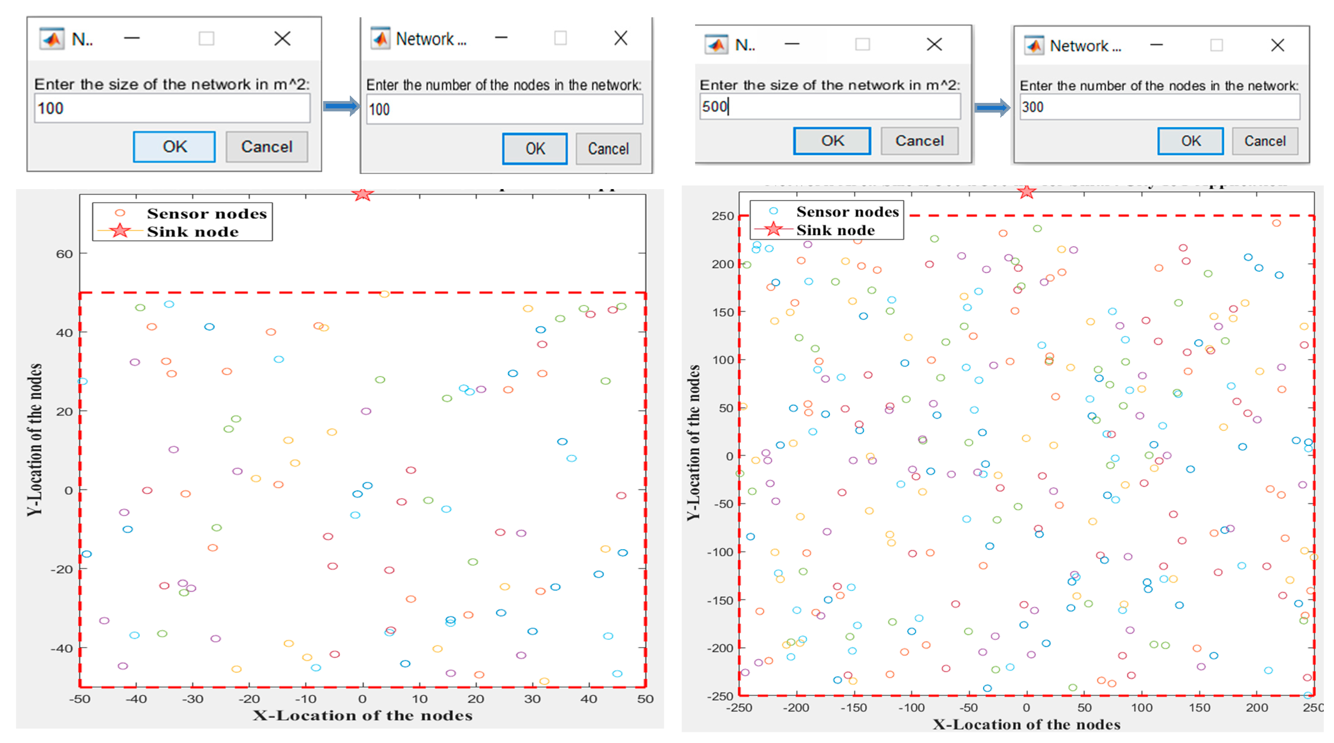
• Every network area size is customized to reflect a particular IoT application.
• There is an abundance of IoT SNs distributed throughout a rectangular geographic area positioned at random, with one the sink node within the IoT network.
• The sink node is positioned outside the physical boundaries of the network and possesses boundless energy. Furthermore, by broadcasting, the sink node can distribute messages to every SN in the network sensory area.
• Each IoT SN and the sink node have unique IDs and are stationary.
• All SNs have finite energy capacity and are isomorphic. This means that they have the same amount of beginning energy and the same processing capacity.
• Every SN is equipped with GPS and knows not only the coordinates of the sink node but also those of other SNs.
• SNs die when their energy runs out completely.
• SNs may regulate their power at which they transmit data according to how close they are to the receiver.
• SNs are allotted specific transmission slots for data fusion purposes, and within these TSs, SNs always have data to communicate, since our protocol is data-driven (i.e., having continuous data to send), not event-driven.
• The distance between the source and the receiver can be estimated based on the received signal strength.

4.2. Energy Consumption Model

In IoT networks, the primary energy-consuming factor is the SNs using energy to communicate with their designated DFHs and the DFHs expending energy to communicate with the sinks or other DFHs (e.g., routing). Additionally, another significant source of energy consumption is the process of data fusion, where DFHs aggregate and process data received from multiple SNs to reduce the amount of data transmitted further up the network. This involves computational energy costs for operations such as filtering, compressing, and merging data streams, which add to the overall energy expenditure of the network. Consequently, radio energy and channel propagation models, which were previously described in [47,48], are used in our simulations. An R-bit packet requires the transmitter to expend the following energy in order to move over a distance d [47,48]:

$$E_{TX}(R,d)=\left\{\begin{array}{cc}R\times E_{elec}+R\times {\epsilon }_{fs}\times d^2,\hfill & if d<d_o,\\ R\times E_{elec}+R\times {\epsilon }_{mp}\times d^4,\hfill & if d\ge d_o.\end{array}\right.$$

(14)

When an R-bit packet is received, the following energy consumptions occur [47,48]:

$$E_{RX}(R,d)=E_{elec}(R),$$

(15)

where the term E_elec, measured in nJ/bit, in Equations (14) and (15) refers to the energy consumed by the transmitter or receiver electrical circuits per bit. In the multipath fading channel model and the free space model, we utilize ${\epsilon }_{mp}$ and ${\epsilon }_{fs}$, respectively, to quantify the energy consumption per bit of the amplifier. The distance between the transmitter and the receiver is indicated by d. The threshold distance, also known as the crossover distance (d_o), is the point of change between the two communication models previously explained. To determine the value of d_o, we employ the subsequent method [47,48]:

$$do=\sqrt{\left({\epsilon }_{fs}/{\epsilon }_{mp}\right)}.$$

(16)

Moreover, the energy consumed during data aggregation (also referred to as data fusion) can be expressed as follows:

$$E_{DA}=N\times E_{fusion},$$

(17)

where N represents the number of SNs whose data are aggregated by DFH, E_fusion is the energy required to process (aggregate) a single bit of data, measured in nJ/bit/signal, and E_DA stands for total energy consumed for data aggregation. Therefore, if R represents the size of a data packet (in bits) received from each SN, then the total energy consumed for aggregating N SNs’ data packets is as follows:

$$E_{DA}=N\times R\times E_{fusion}.$$

(18)

4.3. Network Model

In the proposed protocol, SNs are randomly distributed inside a W × W rectangle sensing field. Each SN has a distinct ID that can be anywhere between 1 and N, such that SN = {SN₁, SN₂, …, SN_N}. Along with its coordinates in relation to the field center, it also contains location information ($x_i,y_i$). The network model’s graphic representation is displayed in Figure 1. Data from SNs are received by a DFH, and are subsequently routed to the sink node, where the sink node is positioned at a specific location outside the region. The network is broken down into rounds throughout its active lifespan. Setup and steady-state are the two phases that jointly make up the first round. The steady-state phase is all that is included in subsequent rounds. It is noteworthy to mention that regrouping (DFH reselection) must take place after a certain number of rounds (i.e., batch), so the setup and steady-state phases are carried out in the following round. However, successive rounds only comprise the steady-state phase, and the process continues, as confirmed in [49]. The RTs for the proposed protocol are given in Figure 2 and Figure 3, respectively, to ensure the efficiency of the data fusion mechanism. In the setup phase, the sink node employs the MPA to identify DFHs after dividing the sensing area into DFGs. This will be covered in more depth subsequently. In the setup phase, all SNs in the area of sensing receive a request information message from the sink node, and each SN_i responds by sending an information message to the sink node. The ID, current RE, and location of a SN_i are all part of this message. The sink node breaks down the area of sensing into H equal hexagonal groups after receiving this message from all SNs, where the group’s radius is adaptable to the network size. Every DFG can be represented symbolically by DFG_H and is identified by all SNs. Furthermore, after the MPA method is executed, the sink node gathers these data into the sink node’s table message, which contains crucial network information and is subsequently provided to SNs used to identify as a $DF{H}_l\{1<l<H\}$ for each DFG. In addition, the sink node is liable for figuring out the relative RT and assigning each SN_i a specific TDMA TS for packet transmission during the steady state phase. Consequently, it sends its data directly to DFH_l. After transmission, SN_i enters sleep mode to save energy. Then, a DFH_l collects data from all of DFGMs and delivers them directly to the sink node or the next PDFR based on the proposed protocol without routing and with multi-hop routing, respectively.

When a SN_i fails to provide enough energy sufficient to send a packet to the sink node or its DFH, it becomes dead. In these cases, the SN_i is taken off the sink’s table. A disjoin message is broadcast to all SNs in the network sensing area by a DFH when its energy level sags below a predetermined threshold. Furthermore, information about DFGMs and their corresponding RE levels is included in another disjoin message that is sent straight to the sink node. Here, the sink node realizes that, in order to bring about synchronization, the entire network’s regrouping (DFH reselection) procedure is warranted. The proposed protocol involves various forms of messages, detailed as follows: (1) The Request Information Message: A broadcast from the sink node to all SNs, requesting their information. (2) The SN’s information message: A unicast message is sent by each SN_i to the sink node as a reply. The main fields of this message are the SN’s ID, location, and RE. (3) The sink node’s Table Message contains all necessary information about the SNs after network area division and running the MPA. Each SN_i extracts the required fields based on its role from this message, which has two forms: Firstly, the DFGMs table message, including fields specific to SN_i itself such as the SN’s ID, RE, type, status, DFG number, DFG ID, distance to the sink node, distance to its DFH, and message arrival time in sec. Secondly, the DFH table message, in the case of the proposed protocol without routing, detailing a DFH and its DFGMs, contains the SN’s ID, RE, type, status, DFG number, distance to the sink node, and priority of TDMA TS, while the proposed protocol with routing has the same message fields with additional fields for PDFR information such as the next PDFR ID, the distance between it and its PDFH, RE, status, DFG number, distance to the sink node, and priority of TDMA TS. (4) Disjoin message (to sink node): If a DFH’s energy drops below the threshold, it sends this message to the sink node, which is a unicast message containing the DFGMs’ IDs, their RE, and DFH information, to inform the sink node that regrouping is necessary. (5) Disjoin message (to SNs): A DFH broadcasts this message to all SNs, instructing them to cease data transmission to their DFH due to imminent regrouping, thereby ensuring synchronization across the network, regardless of whether a DFH’s energy is below the threshold.

5. The Proposed Protocol

One of the main factors influencing how long a network lasts is how well a node maintains its energy. The network would fail to achieve its targeted operating needs in a shorter amount of time if its rate of energy consumption increased. The proposed protocol may make sure that PDFHs with more energy are chosen by basing the PDFH selection process on the RE of SNs. This choice criterion may increase the network’s overall stability and lengthen its duration of use. Moreover, the PDFH selection procedure can reduce energy consumption by taking the distance to the sink into account. This method guarantees that SNs closer to the sink are prioritized as PDFHs, reducing the need for energy-consuming long-distance transfers. Furthermore, another critical component in PDFH selection is the average distance between DFGMs, which is considered in the proposed protocol. In conclusion, it seems that the proposed protocol presents a viable option for network-wide energy consumption optimization. Through the consideration of node-to-node energy consumption balance, the proposed protocol might potentially prolong the life of IoT networks and lessen early PDFH death. Moreover, they select PDFH by applying the MPA to calculate the DFFF. The substantial interest in MPA within the research community can be attributed to several factors, including its simplicity, applicability, realistic runtime performance, rapid convergence rate, high effectiveness, and capability to address continuous, multi-objective, and binary optimization problems more efficiently than other established algorithms in the field. To emphasize the effectiveness of MPA, we presented its initial application within an IoT domain directly relevant to this research, along with some preliminary results [50,51]. A key differentiator lies in the use of distinct fitness functions: one study applied a three-dimensional fitness function [50], while another used a five-dimensional fitness function [51]. For the proposed protocol without routing, following the PDFH selection process, SNs send their data to their selected PDFH, which aggregates the received data with its own data and then transmits it directly to the sink node, as shown in Figure 1a in the case of the proposed protocol without routing. However, in the case of the proposed protocol with multi-hop routing, PDFH sends the data to PR based on the RDFCF, as demonstrated in Figure 1b. This section provides a comprehensive overview of the algorithms considered to enhance the performance of the proposed protocol. Specifically, Section 5.1 elucidates the method for dividing the network area, while Section 5.2 offers an in-depth explanation of how the MPA is used to select a PDFH, FSDFH, and SSDFH, while Section 5.3 addresses the techniques employed to avoid intra- and inter-DFG interference. In Section 5.4, data transmission using multi-hop routing and innovative RDFCF is demonstrated thoroughly. The communication overhead is presented in Section 5.5. Finally, Section 5.6 deals with the major network impairments.

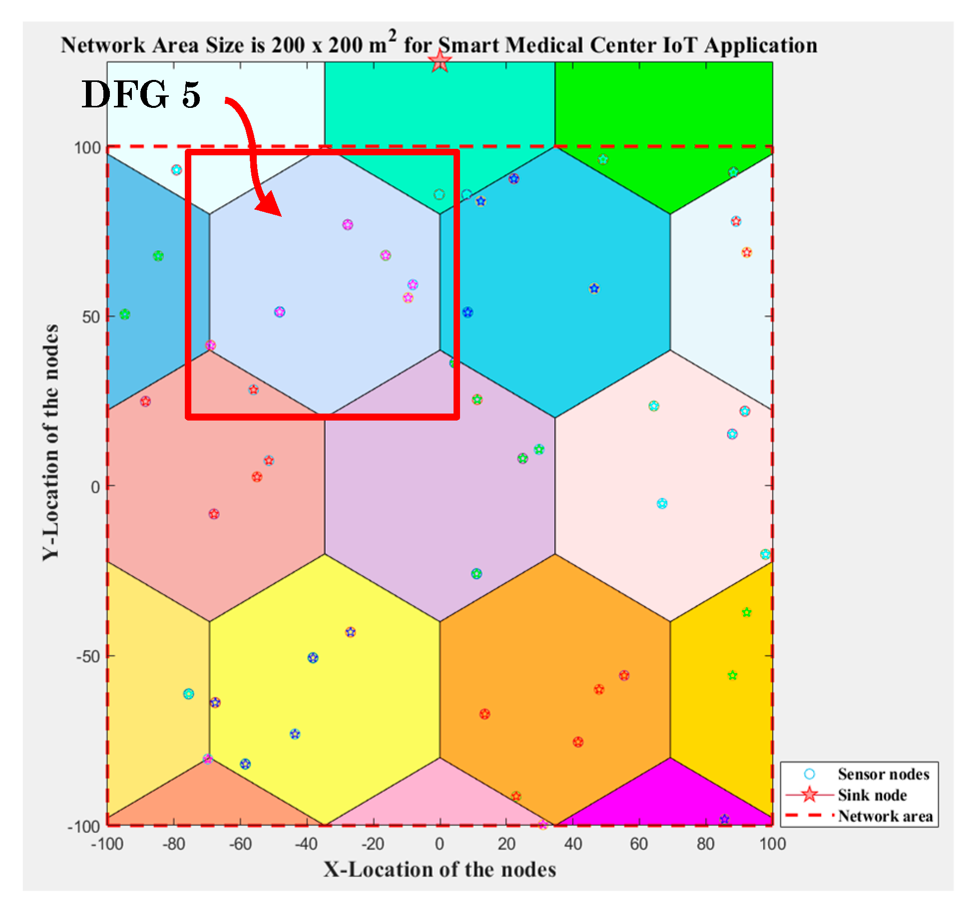
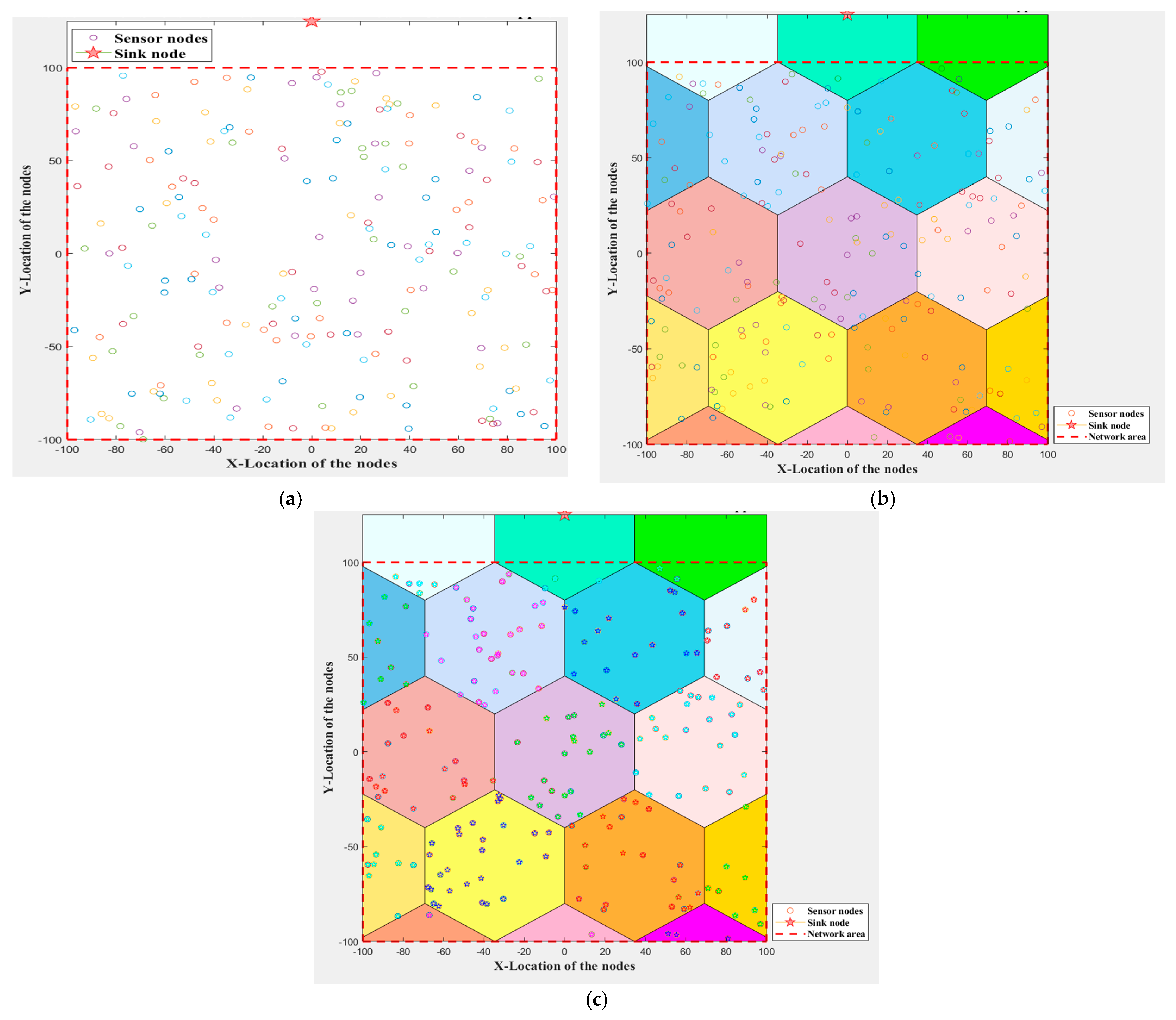
5.1. Network Area Division (DFGs Division)

Hexagonal data fusion grouping ensures uniform coverage, reduces edge effects, and enhances data storage, addressing issues like ungrouped SNs. Unlike circular DFGs, which leave gaps and lead to inefficient space use and irregular neighbor spacing, hexagonal grids offer superior adjacency and clarity, making them ideal for IoT networks. Managing DFGs in IoT networks improves efficiency, scalability, and energy conservation by aggregating data at a central point (i.e., DFH) instead of transmitting it from multiple SNs. This reduces communication load and power consumption, vital for battery-powered SNs. The network sensing area (W × W) is partitioned into hexagonal DFGs of the same size with a pointy top orientation, following a methodology similar to that presented in [32], with density calculated for both the overall network and individual groups. The sink node adjusts DFGs dynamically, aiming for balance between network density and DFG density. If the densities mismatch, merging or redistribution strategies are employed to optimize connectivity, load distribution, and network performance, minimizing redundancy and ensuring efficient operation. Each hexagonal DFG’s side length (S) can be determined by applying the formula given in Equation (19).

$$S=W/f,$$

(19)

where W refers to the network size measured in (m) and f is a constant defined by the simulation.

In the pointy top orientation, the vertical distance (v) between neighboring hexagonal centers is $v=\left({\displaystyle \frac{3}{4}}\right)\times height=\left({\displaystyle \frac{3}{2}}\right)\times S$. However, the horizontal distance (h) is $h=width=\sqrt{3}\times S$, as represented in Figure 4. Based on this division, Figure 5a illustrates the network before partitioning, covering an area of 200 × 200 m². Subsequently, Figure 5b,c demonstrate the network post-partitioning and the distribution of SNs into the constructed DFG.

In our proposed protocol, each network size is representative of a specific IoT application, with an assumed network density of 0.0025 nodes/m², which is also equivalent to a DFG density.

Table 3. Variations in network area sizes and their corresponding details.

Network Size (W)	Hexagonal Side Length (S)	SNs Count (N)	IoT Application Type	The Sink Node Location
100 × 100 m2	20 m	25	Smart logistics park	(0,75)
200 × 200 m2	40 m	100	Smart medical center	(0,125)
300 × 300 m2	60 m	225	Smart factories zone	(0,175)
400 × 400 m2	80 m	400	Smart university	(0,225)
500 × 500 m2	100 m	625	Smart city	(0,275)

provides a comprehensive overview of these applications. Additionally, Figure 6a–e depicts models of a smart logistics park, smart medical center, smart factories zone, smart university, and smart city, along with their corresponding network sizes. Algorithm 1 shows the detailed steps of the setup phase.

Algorithm 1. DFGs formation (setup phase) for the proposed protocol.

5.2. PDFH and SDFH Selection Utilizing the MPA

Because DFHs play a crucial role in routing and data collection, DFH selection is a vital phase in WSN-based IoT, with respect to their role in gathering data from DFGMs and transmitting them to the sink node. Selecting ideal DFHs becomes especially important in networks that are homogeneous, meaning that each SN has the same energy level. It is essential to have this option in order to guarantee that energy utilization is spread uniformly throughout the network [13]. Many strategies, such as GA [52,53], PSO [35,54], fuzzy logic system [55,56], and Equilibrium Optimizer (EO) [31,57], to mention a few, have been developed for CH selection. The proposed protocol impressively incorporates the MPA, an effective and state-of-the-art optimization technique, to identify the optimal PDFH, FSDFH, and SSDFH for each DFG by applying a well-defined DFFF. However, the reason behind selecting FSDFH and SSDFH will be discussed in Section 5.6. The MPA is an innovative metaheuristic algorithm that has proven to be adaptable in solving a variety of real-world issues. One key advantage lies in its ability to mimic the behavior of marine predators, drawing inspiration from their foraging strategies and adaptive capabilities. By leveraging concepts from nature, MPA can effectively navigate complex search spaces, making it well-suited for addressing the PDFH selection problem [58]. Additionally, MPA incorporates mechanisms for exploration and exploitation, allowing it to strike a balance between global exploration and local exploitation. Another advantage is its simplicity and ease of implementation, making it accessible to researchers and practitioners across different domains. Furthermore, MPA’s memory retention mechanism enables it to remember successful solutions, facilitating continuous improvement over successive iterations [44]. The MPA has demonstrated its efficacy in selecting the most optimal PDFH, thereby enhancing energy conservation and prolonging the network’s lifespan in the proposed protocol. In order to accomplish this goal, the communication distance between the sink node and DFGMs in a particular DFG, their RE, average distance between DFGMs, ASBO, and PDFH rotation times are the main RMs that the sink node evaluates to select the finest PDFH based on the DFFF. Figure 7 provides a thorough illustration of the selection process for PDFHs using the MPA.

The data exchange starts with the sink node broadcasting a request information message to every SN. In response to the sink’s message, SNs reply with an information message that carries their own distinct IDs, the coordinates of X and Y, and the current RE. The sink node consequently becomes comprehensive information on each SN. After that, the setup phase is initiated by the sink node, which divides the network sensory area into hexagonal DFGs and places SNs among them. To put it briefly, this study uses the well-known MPA as an optimization method to determine which DFGM is best suited to fulfill the role of a PDFH. As the ensuing subsections shall expound upon, the MPA comprises two phases: the initialization phase and the iteration phase.

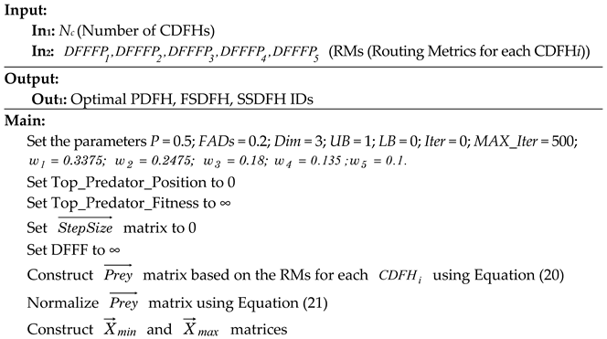
5.2.1. The Initialization Phase

During the initialization phase of the MPA, a set of input parameters needs to be configured, which includes the following:

(a)

Number of search agents (SAs): This parameter represents the number of DFGMS within a certain DFG eligible to participate in the DFH selection process (N_c).

(b)

Dimension (Dim): This parameter defines the number of RMs utilized in our research; its specific value is set at 5.

(c)

Maximum number of iterations (Max_Iter): This parameter involves iteratively running the algorithm to determine the most appropriate DFH node. In our proposed protocol, Max_Iter is defined as 500.

(d)

Lower and upper and bounds (LB and UB): The LB and UB are set to 0 and 1, respectively. Specifically, our proposed protocol utilizes a normalization technique to define these boundaries at 0 and 1. This choice arises from the lack of precise information regarding the UB and LB of the three RMs employed in our study. To ensure equal treatment and establish uniformity among these metrics, we opted for normalization. As a result, all values are confined within the standardized range of [0, 1].

(e)

Positions: This parameter comprises an array of IDs corresponding to the DFGMs located within a DFG, utilized to identify the optimal DFH’s ID.

(f)

Main parameters of MPA: The authors in [43] have defined these parameters (i.e., FADs and P), which have the values of 0.2 and 0.5, respectively. Interestingly, these values are retained and unchanged in our study. The following are the initial values that will be subject to updates in subsequent phases.

$$Top\_predator \_pos=[0 0 0 0 0], Top\_predator \_fit=\infty$$

$$\overrightarrow{\mathrm{S}tepSize}=\begin{array}{c}\begin{array}{c}S{A}_1\\ S{A}_2\\ :\\ S{A}_{Nc}\end{array}\end{array}\left[\begin{array}{ccccc}0& 0& 0& 0& 0\\ 0& 0& 0& 0& 0\\ :& :& :& :& :\\ 0& 0& 0& 0& 0\end{array}\right], \overrightarrow{fitness}=\begin{array}{cc}\begin{array}{c}S{A}_1\\ S{A}_2\\ :\\ S{A}_{Nc}\end{array}& \left[\begin{array}{c}0\\ 0\\ :\\ 0\end{array}\right]\end{array}$$

$${\overrightarrow{X}}_{\min }=\begin{array}{c}\begin{array}{c}S{A}_1\\ S{A}_2\\ :\\ S{A}_{Nc}\end{array}\end{array}\left[\begin{array}{ccccc}0& 0& 0& 0& 0\\ 0& 0& 0& 0& 0\\ :& :& :& :& :\\ 0& 0& 0& 0& 0\end{array}\right], {\overrightarrow{X}}_{\max }=\begin{array}{c}\begin{array}{c}S{A}_1\\ S{A}_2\\ :\\ S{A}_{Nc}\end{array}\end{array}\left[\begin{array}{ccccc}1& 1& 1& 1& 1\\ 1& 1& 1& 1& 1\\ :& :& :& :& :\\ 1& 1& 1& 1& 1\end{array}\right]$$

(g)

$\overrightarrow{Prey}$ matrix generation: This matrix is the initial solution for the MPA. A DFG is thought to have a list of DFGMs, each of which is expected to be a Candidate DFH (CDFH) and it is identified as CDFH = [CDFH₁, CDFH₂, …, CDFH_Nc], where Nc represents the number of rows in $\overrightarrow{Prey}$ matrix. On the other hand, each DFGM has five RMs, which indicate the number of columns for the $\overrightarrow{Prey}$ matrix and can be written as RM = [RM₁, RM₂, RM₃, RM₄, RM₅], where RM₁ refers to the distance between a CDFH_i and the sink ($D_{CDF{H}_i\to Sink}$), RM₂ denotes for the ratio of the initial energy to the current RE of a CDFH_i $Inv(R{E}_{CDF{H}_i})$, RM₃ is the average distance between DFGMs ($AvgDi{s}_{CDF{H}_i\to DFGMs}$), RM₄ stands for the ratio of the average number of times (either rounds or batches) that all IoT SNs have become DFHs (i.e., assigned the DFH role) to the number of times (either rounds or batches) CDFH_i played this role $X_{CDF{H}_i}$, and RM₅ represents $ASB{O}_{CDF{H}_i}$. The exact definitions of these RMs will be thoroughly discussed later, as shown in Equation (20).

$$\overrightarrow{Prey}=\begin{array}{cc}& \begin{array}{ccccc}\hspace{1em}\hspace{1em}\hspace{1em}{\mathrm{RM}}_1\hspace{1em}\hspace{1em}\hspace{1em}& \hspace{1em}\hspace{1em}{\mathrm{RM}}_2\hspace{1em}\hspace{1em}\hspace{1em}\hspace{1em}& \hspace{1em}\hspace{1em}\hspace{1em}{\mathrm{RM}}_3\hspace{1em}\hspace{1em}\hspace{1em}\hspace{1em}\hspace{1em}& {\mathrm{RM}}_4\hspace{1em}\hspace{1em}\hspace{1em}& \hspace{1em}{\mathrm{RM}}_5\hspace{1em}\hspace{1em}\hspace{1em}\end{array}\\ \begin{array}{c}{CDFH}_1\\ {CDFH}_2\\ \begin{array}{c}:\\ .\end{array}\\ {CDFH}_{Nc}\end{array}& {\left[\begin{array}{c}\begin{array}{ccccc} \hspace{1em}{D_{{CDFH}_1\to Sink}}_{(1,1)}\hspace{1em}& {Inv(R{E}_{CDF{H}_1})}_{(1,2)}& \hspace{1em}{{AvgDis}_{{CDFH}_1\to DFGMs}}_{(1,3)}& \hspace{1em}{X}_{{CDFH}_1(1,4)}& \hspace{1em}{ASBO}_{{CDFH}_1(1,5)}\end{array}\\ \begin{array}{ccccc}\hspace{1em} {D_{{CDFH}_2\to Sink}}_{(2,1)}\hspace{1em}& {Inv(R{E}_{CDF{H}_2})}_{(2,2)}& \hspace{1em}{{AvgDis}_{{CDFH}_2\to DFGMs}}_{(2,3)} & X_{{CDFH}_2(2,4)}& \hspace{1em}{ASBO}_{{CDFH}_2(1,5)}\end{array}\\ \begin{array}{ccc}\hspace{1em}:\hspace{1em}\hspace{1em}\hspace{1em}\hspace{1em}\hspace{1em}\hspace{1em}\hspace{1em}& :\hspace{1em}\hspace{1em}\hspace{1em}\hspace{1em}& \hspace{1em}\hspace{1em}\hspace{1em}\hspace{1em}:\hspace{1em}\hspace{1em}\hspace{1em}\hspace{1em}\hspace{1em}\hspace{1em}\hspace{1em}\hspace{1em}:\hspace{1em}\hspace{1em}\hspace{1em}\hspace{1em}\hspace{1em}\hspace{1em}:\end{array}\\ \begin{array}{ccccc}\hspace{1em} {D_{{CDFH}_{\mathit{Nc}}\to Sink}}_{(\mathit{Nc},1)}& {Inv(R{E}_{CDF{H}_{Nc}})}_{(Nc,2)}& {{AvgDis}_{{CDFH}_{Nc}\to DFGMs}}_{(Nc,3)}& X_{{CDFH}_{Nc}(Nc,4)}& {ASBO}_{{CDFH}_{Nc}(Nc,5)}\end{array}\end{array}\right]}_{Nc\times 5}\end{array}$$

(20)

It is good to stress the point that the $\overrightarrow{Prey}$ matrix is normalized. In other words, every RM performs a normalization process. By using this method, the values of RMs are rescaled to fall inside the [0, 1] range. In order to ensure impartiality and meaningful comparisons amongst the many criteria while identifying the best DFH, this normalizing step is essential. Equation (21) provides a detailed description of the particular normalization procedure. Assuming that a RM is in the “m” row and is in the “n” column, we can say that RM_scaled reflects the scaled RM version of the original RM after normalization.

$$R{M}_{scaled}={\displaystyle \frac{R{M}_{m,n}-R{M}_{n(\mathit{min})}}{R{M}_{n(\mathit{max})}-R{M}_{n(\mathit{min})}}},$$

(21)

where m values are located in [1, N_c], n has five values (1, 2, 3, 4, and 5), RM_m,n stands for the original value of RM that requires normalization, and RM_n(max) and RM_n(min) are the maximum and minimum values of the RM in the same column, respectively.

5.2.2. The Iterative Phase

The DFFF will be used in this phase to determine which DFH is chosen. We also comprehend that the DFFF is essential to tracking down and identifying the prey (target node) in the MPA process. This subsection introduces the DFFF’s parameters before being followed by a powerful DFFF.

• DFFF parameters definitions

The MPA’s process of choosing the best DFH depends substantially on the definition of the relevant DFFF. To achieve this, we have incorporated $D_{CDF{H}_i\to Sink}$, a shorter distance to the sink node, less $AvgDi{s}_{CDF{H}_i\to DFGMs}$, more RE levels, a smaller ASBO, and a smaller number of PDFH rotations into the proposed DFFF. The purpose of the DFFF is to prolong the network’s lifetime and reduce energy consumption. This subsection provides a comprehensive description of the DFFF parameters:

(1)

The ratio of CDFH_j’s initial energy (E_o) to its current RE ($R{E}_{CDF{H}_i}$) $Inv(R{E}_{CDF{H}_i})$: This metric represents the amount of energy left in the DFGMs after they have been in operation. When choosing a DFH, this is the most important parameter to take into account. Due to its collection, aggregation, and transmission of DFGMs data to the sink node, DFH uses a disproportionate amount of energy as compared to other SNs. The DFFF Parameter ($DFFF{P}_1$) is a representation of this parameter, and it should be minimized. Also, as a result of the normalizing procedure, its value falls between 0 and 1, as shown in Equation (22). This parameter guarantees that a CDFH_j with more RE is selected to be a DFH.

$$DFFF{P}_1=Inv(R{E}_{CDF{H}_i})=E_{o_{CDF{H}_i}}/R{E}_{CDF{H}_i},\hspace{1em}0<DFFF{P}_1<1.$$

(22)

(2)

Distance of the CDFH_j to the sink node ($D_{CDF{H}_i\to Sink}$): This parameter is symbolized by $DFFF{P}_2$ and it needs to be reduced to shorten the transmission’s overall distance. Equation (21) illustrates how the normalization process triggers its value to be from 0 to 1.

$$DFFF{P}_2=D_{CDF{H}_i\to Sink},\hspace{1em}0<DFFF{P}_2<1.$$

(23)

Using Euclidean distance, $DFFF{P}_2$ determines which DFGM is most suited to become a DFH depending on how close CDFH_j is to the sink node. Equation (24) is used to compute $D_{CDF{H}_i\to Sink}$.

$$D_{{CCH}_i\to Sink}=\sqrt{{({sink}_y-{{CCH}_i}_y)}^2+{({sink}_x-{{CCH}_i}_x)}^2}.$$

(24)

(3)

Average distance between DFGMs ($AvgDi{s}_{CDF{H}_i\to DFGMs}$): This parameter is the measure of how centered a CDFH_j is in relation to all of its neighbors (DFGMs). This is an essential first step towards reducing intra-DFG communication costs. DFGMs use less energy to transfer data to DFHs if DFHs have lower $AvgDi{s}_{CDF{H}_i\to DFGMs}$ values. Therefore, $AvgDi{s}_{CDF{H}_i\to DFGMs}$ is denoted by $DFFF{P}_3$. Moreover, this function should be minimized. Additionally, the distance between CDFH_j and its neighbor CDFH_j is determined using Euclidean distance, as demonstrated in Equation (25).

$$DFFF{P}_3=AvgDi{s}_{CDF{H}_i\to DFGMs}={\displaystyle \frac{1}{Nc-1}}{\displaystyle \sum _{j=1,j\ne i}^{Nc}(D_{CDF{H}_j\to CDF{H}_i}),}\hspace{1em}0<DFFF{P}_3<1.$$

(25)

$$D_{{CDFH}_j\to {CDFH}_i}=\sqrt{{({{CDFH}_j}_y-{{CDFH}_i}_y)}^2+{({{CDFH}_j}_y-{{CDFH}_i}_x)}^2}.$$

(26)

(4)

$X_{CDF{H}_i}$: This parameter refers to the ratio of the number of times (either rounds or batches) that the current CDFH_j played the DFH role to the average number of times (either rounds or batches) that all DFGMs have become DFHs (i.e., assigned the DFH role). Therefore, $X_{CDF{H}_i}$, which also known as $DFFF{P}_4$ can be expressed as follows:

$$DFFF{P}_4=X_{CDF{H}_i}=DFH{R}_{CDFC{H}_i}/\left({\displaystyle \frac{{\displaystyle \sum _{k=1}^{N_c}DFH{R}_{CDF{H}_k}}}{N_c}}\right), 0<DFFF{P}_4<1.$$

(27)

where $DF{R}_{CDF{H}_k}$ refers to the number of times (either rounds or batches) that a CDFH k is assigned the DFH role.

(5)

Average scale for buildings occlusions ($ASB{O}_{CDF{H}_i}$): ASBO refers to an estimation that represents the extent to which buildings obstruct visibility or line-of-sight in a given area. This scale can be used to assess factors like sunlight exposure, view obstruction, and even the impact on wireless signal propagation. ASBO is typically calculated by analyzing how much of a particular area or viewpoint is blocked by surrounding buildings. This parameter exemplifies a CDFH_j position (height) to the height of buildings around a PDFH as shown in

Table 4. Representation of building occlusions based on a PDFH position.

Range		Interpretation
	$0-1/3r$	Extremely close
	$1/3r-2/3r$	Close
	$2/3r-r$	Moderately close
	$r-1 1/3r$	Moderately far
	$1 1/3r-1 2/3r$	Far
	$1 2/3r-2r$	Extremely far

and Figure 8. As a result, $ASB{O}_{CDF{H}_i}$, which also stands for $DFFF{P}_5$, can be defined as follows:

$$DFFF{P}_5=ASB{O}_{CDF{H}_i}={\displaystyle \frac{{\displaystyle \sum _{i=1}^{N_b}SB{O}_{CDF{H}_i}}}{N_b}},\hspace{1em}0<DFFF{P}_5<1.$$

(28)

where $SB{O}_{CDF{H}_i}$ signifies the scale for building occlusions for each CDFH_j, and N_b is assigned to the number of buildings that may occlude CDFH_j within the coverage area. To elaborate more on this,

Table 5. The scale for building occlusions at low height.

Scale	Interpretation
0.1	Extremely close
0.2	Close
0.3	Moderately close
0.4	Moderately far
0.5	Far
0.6	Extremely far

,

Table 6. The scale for building occlusions at moderate height.

Scale	Interpretation
0.2	Extremely close
0.3	Close
0.4	Moderately close
0.5	Moderately far
0.6	Far
0.7	Extremely far

and

Table 7. The scale for building occlusions at high height.

Scale	Interpretation
0.3	Extremely close
0.4	Close
0.5	Moderately close
0.6	Moderately far
0.7	Far
0.8	Extremely far

represent the interpretations for the scale. In essence, the scale preference indicates that lower is better.

• DFFF estimation:

In order for the MPA to locate the best PDFH and FSDFH, one essential element is the DFFF. To discover a feasible solution, the MPA takes into account all of the aforementioned parameters when designing the DFFF. It is important to note that the CDFH_i that has the lowest DFFF is selected to be PDFH, and the second lowest one is nominated as FSDFH. Thus, the following is the best linear combination of DFFFP₁, DFFFP₂, DFFFP₃, DFFFP₄, and DFFFP₅ for PDFH and FSDFH selection:

$$DFFF=w_1\times DFFF{P}_1+w_2\times DFFF{P}_2+w_3\times DFFF{P}_3+w_4\times DFFF{P}_4+w_5\times DFFF{P}_5,$$

(29)

where $w_1$, $w_2$,$w_3$, $w_4$, and $w_5$ stand for the weight’s values for RM₁, RM₂, RM₃, RM₄, and RM₅, respectively, where $w_1+w_2+w_3+w_4+w_5=1.$ The values of $w_1$, $w_2$,$w_3$, $w_4$, and $w_5$ are 0.3375, 0.2475, 0.18, 0.135, and 0.1, respectively. It is important to stress that an extensive amount of trial-and-error evaluation goes into determining these precise values. While Appendix A offers a thorough and informative example that clarifies the PDFH, FSDFH, and SSDFH selection process using the MPA, Algorithm 2 depicts the all-inclusive MPA-based PDFH and SDFH selection procedure.

Algorithm 2. PDFH, FSDFH, and SSDFH selection using the MPA in the proposed protocol.

5.2.3. Optimizing Data Fusion Regrouping (PDFH Reselection) Procedure

Indeed, to guarantee that the PDFH selection process is not carried out in each round, in this paper, once the sink node selects PDFH of each DFG using the MPA at the initial round, the process of regrouping for the next round is decided locally by each PDFH that is currently in place (i.e., distributed-based). The proposed protocol requires PDFHs to compare their RE levels (RE_PDFH) to the energy threshold ($E_{th}$) in the subsequent round after the setup phase. Equation (30), which represents the $E_{th}$, defines it as the average RE of all DFGMs, including PDFH. If the RE_PDFH is equal to or greater than the $E_{th}$, PDFH can continue to communicate inside the DFG with DFGMs; if not, it must stop and send a disjoin message to the sink node and all SNs in the network to choose a new PDFH as per Equation (31). This message contains the current RE levels of DFGMs.

$$E_{th}={AVG\_RE}_{(DFGMs)}=\left({\displaystyle \sum _{j=1}^{N_c}RE(j)}/N_c\right) .$$

(30)

$$\mathrm{PDFH} \mathrm{reselection} =\left\{\begin{array}{cc}\mathrm{Seleect} \mathrm{a} \mathrm{new}\mathrm{PDFH},\hfill & \mathrm{if} E_{th}>R{E}_{PDFH}\\ \mathrm{Keep} \mathrm{the} \mathrm{current} \mathrm{PDFH},\hfill & \mathrm{if} E_{th}<R{E}_{PDFH}\end{array}\right..$$

(31)

This technique reduces the number of control overhead during the setup phase (i.e., PDFH selection) by ensuring that the proposed protocol ensures that the PDFH selection procedure is not repeated for each round. Before PDFHs may be re-selected, the RE of the chosen PDFHs must drop to a certain level. When the subsequent eligible DFGM is selected to act as PDFH, the reselection process is considered satisfactory. As a result, PDFH can stay the same for several rounds until its RE drops below $E_{th}$. That is why our protocol is considered batch-based. This condition is necessary to prevent PDFH from disconnecting the network and dying prematurely. An additional feature is suggested in the proposed protocol for setting a dynamic threshold for the RE, ensuring that SNs will stay qualified for PDFHs until the network has totally broken down. In other words, $E_{th}$ is calculated each round, and its value changes based on the current RE of the DFGMs, as specified in Equation (30). As can be observed from the results presented in Section 6, this aspect significantly improves the network’s longevity over traditional approaches.

When RE_PDFH drops below $E_{th}$, they are degraded to DFGMs so that they may carry on with their sensing duties. A new PDFH is chosen to replace the existing one in light of the RMs values and the MPA. The network also removes dead SNs. Since PDFHs need to be awake all the time, this increases the amount of energy they need. SNs rotate PDFHs in order to maintain equilibrium in energy consumption. Algorithm 3 demonstrates the PDFH selection and reselection procedures for the proposed protocol.

Algorithm 3. PDFH selection and reselection procedures for the proposed protocol.

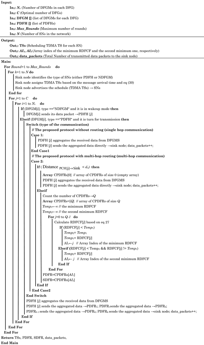
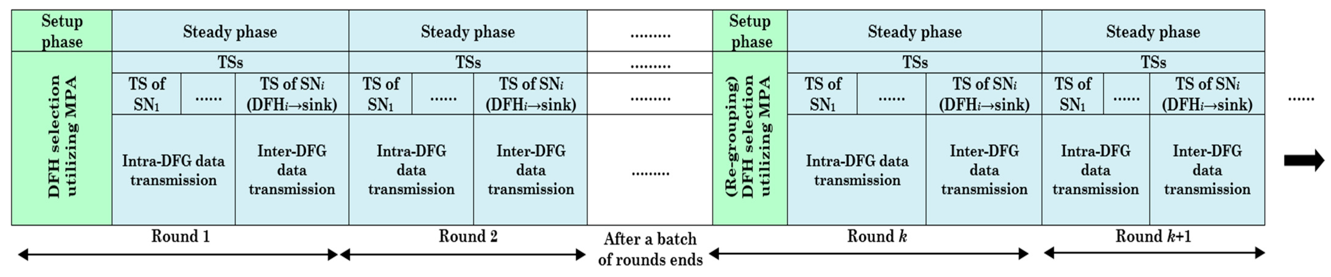
5.3. Mastering Data Fusion Communications: Efficient Scheduling and Transmission over Intra- and Inter-DFG

As was previously pointed out, SNs reply with information messages after receiving a request for information from the sink node. The arrival time of each message received by SNs is then recorded by the sink node for usage at an ulterior point and time. Consequently, the sink node divides the network area into identical hexagonal DFGs and begins the process of PDFH, FSDFH, and SSDFH selection by running the MPA between DFGMs in each DFG. After determining PDFHs, FSDFHs, and SSDFHs, the sink node sends the sink’s table message for all SNs in the network containing its ID, arrival time, its role (PDFH or DFGM), DFG number, PDFH ID, their TSs, and distance to the sink and to PDFH. After SNs receive the sink’s table message, the steady-state phase starts. In simpler terms, SNs send their data to their PDFHs, which in turn send the data to the sink node, which maintains sufficient knowledge about all PDFH IDs and DFGMs that correspond with them, aside from DFG ID, RT, and the message arrival time for all SNs. Therefore, the sink is in charge of assigning TDMA TSs for SNs. In-depth explanations of the workings of this scheduling strategy will be covered shortly. In fact, the TDMA schedule that is suggested in [59] is enhanced by TDMA, which makes use of neighborhood data from the local area to efficiently arrange TSs and reduce the likelihood of collisions. The selected PDFH controls the data fusion and transmission process by acting as a control center inside its local region (i.e., DFG). In addition, the sink creates a TDMA schedule for the DFG’s DFGMs, giving each one a specific TS for data transmission during the steady-state phase. With this scheduling technique, intra-DFG interference is evaded, and data collisions inside the DFG are avoided since SNs only send data during their assigned TS. Additionally, this technique makes it easier for DFGMs to adopt a sleep–wake cycle. In order to preserve energy during their sleep cycles, SNs must be active only during their allotted TDMA TSs throughout this cycle. SNs may run at a reduced rate of power during the sleep cycle to effectively conserve energy. PDFH gathers sensed data from all DFGMs within their allotted TSs at the completion of each round (i.e., steady-state phase), aggregates these data, and then sends the aggregated data back to the sink node via single-hop or multi-hop communication channels. No matter how many data packets are received in PDFHs, they aggregate the received data packets into a single packet, therefore lowering the volume of data and directly sending the fused data to the sink node. Indeed, the use of Direct Sequence Spread Spectrum (DSSS) for communication between the sink node and PDFH is crucial. Specifically, DSSS is employed to minimize inter-DFG interference. Each DFG is assigned a unique spreading code that differs from those used in adjacent DFGs. This distinct spreading code effectively prevents inter-DFG interference, ensuring that DFGs do not interfere with each other. To provide further light on how TDMA performs in the proposed protocol without routing, each DFGM within a DFG is given a ranking order by the sink node based on the information message’s arrival time once the data fusion grouping procedure is complete. “First reach, first assign” is the mechanism used in ranking if the type of DFGM is Normal DFGM (“NDFGM”). This concept states that the first information transmission to reach PDFH is ranked 1, the second arrival is ranked 2, and so on. Until each NDFGM in the DFG is given its proper ranking order, this ranking process is completed. Conversely, because PDFH receives data from DFGMs, aggregates them with its own data, and then transmits the fused data to the sink node, it is given the highest rank in the DFG regardless of its arrival time. Due to this fact, the sink node now uses the TDMA scheduling approach to assign transmission TSs. The allocation criteria are based on the given rank, which is saved in the Turn of TDMA TS field. Additionally, the precise allocated TS is expressed by Equation (32), and the arrangement of intra- and inter-DFG TSs for a single DFG, such as DFG 6, is shown in

Table 8. TDMA schedule for intra and inter for DFG 6.

SN ID	Message Arrival Time (ms)	Type	DFG ID	PDFH ID	Rank	TDMA TS Number
20	10	“NDFGM”	6	10	1	1
16	15	“NDFGM”	6	10	2	2
4	16	“NDFGM”	6	10	3	3
32	20	“NDFGM”	6	10	4	4
10	7	“PDFH”	6	10	5	5

.

$$TS=\left\{\begin{array}{cc}{\displaystyle \frac{RT}{N_c+1}},\hfill & if sin\mathrm{gle}-\mathrm{hop} \mathrm{communication} \mathrm{is} \mathrm{employed},\\ {\displaystyle \frac{RT}{N_c+N_{PDFRs}+1}},& if \mathrm{multi}-\mathrm{hop} \mathrm{communication} \mathrm{is} \mathrm{employed},\end{array}\right.$$

(32)

where $N_{PDFRs}$ refers to the number of PDFRs needed to reach the sink node.

5.4. Transmission Through Multiple Hops Using an Innovative Relay Data Fusion Cost Function for Improving Routing Technique

In IoT networks, data fusion is essential for addressing energy consumption challenges, particularly given the energy limitations of SNs. By aggregating and processing raw data locally within the network, data fusion minimizes the amount of data that needs to be transmitted, thereby reducing the energy required for communication, which is directly influenced by packet size and transmission distance. It eliminates redundant data, ensuring that only relevant information is transmitted, and enables localized processing, reducing the reliance on long-distance communication, which consumes exponentially more energy. These efficiencies extend the lifespan of SNs and the network as a whole, making IoT deployments more sustainable and scalable, particularly in energy-sensitive or remote environments where battery replacement is impractical. Data fusion, therefore, plays a critical role in optimizing energy use and enhancing the overall efficiency of IoT systems. In the proposed protocol without routing, PDFHs directly forward the collected data to the sink node after aggregating it from SNs. As a result, PDFHs farther away from the sink node consume more energy and die far sooner than PDFHs closer to the sink. To achieve reliable and effective load balancing and reduce the overhead of communication (i.e., transmission distances), we provide the idea of multi-hop communication to the proposed protocol. It is interesting to note that a DFG-based method is incorporated into an effective multi-hop communication process, in which PDFHs independently gather data from every SN in their DFGs and forward it to the sink node. To effectively send the gathered data to the sink node, PDFHs essentially use intermediary PDFHs as PDFRs, FSDFRs, and SSDFRs. Section 5.5 will go into further information about the function of FSDFRs and SSDFRs. The multi-hop approach employed in the proposed protocol offers reliable, stable, and efficient load balancing by minimizing transmission distances. Taking into account the previous discussion, the proposed protocol has two different types of communication processes: intra-DFG communication and inter-DFG communication. A PDFH and a SDFH are allocated to each DFG when the network is divided into many DFGs for multi-hop inter-DFG communication. PDFH is responsible for managing intra-DFG communication, or communications between DFGMS within that DFG. Part of this PDFH’s function is to collect data from DFGMs within its DFG and, based on how far away from the sink node it is, send it there directly if the distance is less than d_o, or through an intermediary PDFH (PDFRs and SDFRs) if the distance is greater. In the proposed protocol, the sink node performs the computations required to determine which PDFRs and SDFRs are optimal for each PDFH.

This approach significantly enhances inter-DFG communications in scenarios where PDFHs and the sink node are located at significant distances from one another. This reduces energy consumption and increases the network’s operational lifetime. Crucially, when selecting a PDFR and a SDFR, the prerequisites that follow must be fulfilled: (1) The Euclidean distance between Candidate PDFR (CPDFR) and PDFH should be as near to d_o as possible in the direction of the sink node (i.e., upstream), provided that it is smaller than d_o. The numerator of Equation (33), which is carefully chosen to make certain that the smallest value is the ideal one, provides this assurance. (2) In the upstream direction, the CPDFR should have the greatest RE among all PDFHs; to maintain this, the average RE of all CPDFRs is divided by the RE of CPDFR j. (3) $ASB{O}_{CPDFRs\left[j\right]}$ is also considered based on Table 4, Table 5, Table 6 and Table 7, Figure 8, and Equation (23). This leads to the proposal of an innovative RDFCF, whereby each PDFH chooses SR with the second-lowest RDFCF and PDFR with the lowest. Until the data reaches the sink node, the process is then repeated. For this reason, the RDFCF of a CPDFR j ($RDFCF [j]$) is estimated as follows:

$$RDFCF[j]=\left({\displaystyle \frac{do}{D_{PDF{H}_i\to CPDFRs\left[j\right]}}}\right)+\left({\displaystyle \frac{Avg\left(R{E}_{CPDFRs\left[K\right]}\right)}{R{E}_{CPDFRs\left[j\right]}}}\right)+\left({\displaystyle \frac{Avg\left(ASB{O}_{CPDFRs\left[K\right]}\right)}{ASB{O}_{CPDFRs\left[j\right]}}}\right),\hspace{1em}j=0,1,2,....,K-1,$$

(33)

where $D_{PDF{H}_i\to CPDFRs\left[j\right]}$ is the distance between CPDFRs[j] and PDFH_i, each of which represents a distinct member of the CPDFRs array. Conversely, $Avg(R{E}_{CPDFRs\left[K\right]})$ represents the average RE of all CPDFRs, and $R{E}_{CPDFRs\left[j\right]}$ indicates the RE of CPDFRs[j]. By doing this, the multi-hop routing approach utilized in this work increases the effectiveness of communication in situations where there are considerable distances between PDFHs and the sink node, without using unnecessary energy during the communication process, thereby extending the lifetime of the network. Furthermore, the integration of data fusion plays a pivotal role in this context. Data fusion allows intermediate PDFRs to aggregate and synthesize incoming data from multiple sources, significantly reducing redundant transmissions. This process minimizes the amount of raw data forwarded to the sink node, conserving energy at each hop and reducing network congestion. As a result, the overall efficiency of the communication process improves, further extending the network’s lifetime. Algorithm 4 provides a more thorough description of how the proposed protocol operates for scheduling, data transmission, and leveraging data fusion for optimized performance.

Algorithm 4. Scheduling and data transmission for the proposed protocol.

5.5. Communication Overhead of the Proposed Protocol

In this subsection, we aim to provide readers with a comprehensive demonstration of how our network model manages energy dissipation. In essence, the radio and channel propagation models for energy consumption are applied in this paper, which were previously described in [47,48]. The energy used in the proposed protocol is broken down into two phases: setup energy and steady-state energy.

• The first round, which involves both setup and steady-state phases, proceeds as follows:

✓

Setup phase:

1.

The sink node sends a request information message to each SN. Thus, the energy dissipated by each SN to receive the request information message is as follows:

$$E_{RSNs}(N{L}_C,d_{SN\to sink})=E_{elec}\times N{L}_C,$$

(34)

where $N{L}_C$ represents the length of control message.

2.

The energy dissipated by each SN in order to send their information message to the sink node.

$$E_{TSNs}(N{L}_C,d_{SN\to sink})=\left\{\begin{array}{c}N{L}_C\times E_{elec}+N{L}_C\times {\epsilon }_{fs}\times d_{SN\to sink}^2, if d_{SN\to sink}<d_o,\\ N{L}_C\times E_{elec}+N{L}_C\times {\epsilon }_{mp}\times d_{SN\to sink}^4, if d_{SN\to sink}\ge d_o.\end{array}\right.$$

(35)

3.

The energy dissipated by each SN to receive the sink table message.

$$E_{RSNs}(N{L}_C,d_{SN\to sink})=E_{elec}\times N{L}_C.$$

(36)

Thus, the energy dissipated in the setup phase ($E_{Setup}$) is as follows:

$$E_{Setup}=2\times N{E}_{RSNs}+N{E}_{TSNs}.$$

(37)

✓

Steady-state phase:

1.

The energy dissipated by SNs, within a DFG, to send their data to a PDFH.

$$E_{TSNs}(N{L}_D,d_{SN\to PDFH})=\left\{\begin{array}{c}N{L}_D\times E_{elec}+N{L}_D\times {\epsilon }_{fs}\times d_{SN\to PDFH}^2, if d_{SN\to PDFH}<d_o,\\ N{L}_D\times E_{elec}+N{L}_D\times {\epsilon }_{mp}\times d_{SN\to PDFH}^4, if d_{SN\to PDFH}\ge d_o,\end{array}\right.$$

(38)

where $N{L}_D$ represents the length of data message.

2.

The energy dissipated by a PDFH to receive the data from DFGMs, aggregate all the data, including PDFH, and then send them back to the sink node.

$$E_{RPDFH}(N{L}_D,d_{SN\to PDFH})=(N_c-1)\times N{L}_D\times E_{elec}.$$

(39)

$$E_{DAPDFH}(N{L}_D,d)=N_c\times N{L}_D\times E_{fusion}.$$

(40)

$$E_{TPDFH}(N{L}_D,d_{PDFH\to sink})=\left\{\begin{array}{c}N{L}_D\times E_{elec}+N{L}_D\times {\epsilon }_{fs}\times d_{PDFH\to sink}^2, if d_{PDFH\to sink}<d_o,\\ N{L}_D\times E_{elec}+N{L}_D\times {\epsilon }_{mp}\times d_{PDFH\to sink}^4, if d_{PDFH\to sink}\ge d_o.\end{array}\right.$$

(41)

Accordingly, the total energy dissipated by all PDFHs is denoted as follows:

$$E_{PDFHs}=C\times (E_{RPDFH}+E_{DAPDFH}+E_{TPDFH}).$$

(42)

3.

In the subsequent rounds, if the energy of a PDFH is higher than the energy of its DFG, only the steady-state phase is in effect. However, if the energy of a PDFH falls below a DFG’s average energy, regrouping is initiated. During regrouping, the sink node retains information about the SNs’ locations but lacks real-time data on their current energy levels. The sources of energy dissipation in this scenario include the following:

i.

The energy dissipated by all PDFHs to send disjoin messages to the sink node.

$$E_{TCH}(N{L}_C,d_{PDFH\to sink})=\left\{\begin{array}{c}N{L}_C\times E_{elec}+N{L}_C\times {\epsilon }_{fs}\times d_{PDFH\to sink}^2, if d_{PDFH\to sink}<d_o,\\ N{L}_C\times E_{elec}+N{L}_C\times {\epsilon }_{mp}\times d_{PDFH\to sink}^4, if d_{PDFH\to sink}\ge d_o.\end{array}\right.$$

(43)

ii.

The energy dissipated by a PDFH to send disjoin messages to SNs.

$$E_{TCH}(N{L}_C,d_{SN\to PDFH})=\left\{\begin{array}{c}N{L}_C\times E_{elec}+N{L}_C\times {\epsilon }_{fs}\times d_{SN\to PDFH}^2, if d_{SN\to PDFH}<d_o,\\ N{L}_C\times E_{elec}+N{L}_C\times {\epsilon }_{mp}\times d_{SN\to PDFH}^4, if d_{SN\to PDFH}\ge d_o.\end{array}\right.$$

(44)

iii.

The energy dissipated by SNs to receive disjoin messages from a PDFH.

$$E_{RSNs}(N{L}_C,d)=E_{elec}\times N{L}_C.$$

(45)

Consequently, the energy dissipated for the disjoin message is calculated as follows:

$$E_{disjoin}=C\times E_{TCHs}+N\times E_{TCHs}+N\times E_{RSNs}.$$

(46)

Thus, the energy dissipated in the steady-state phase ($E_{Steady}$) is as follows:

$$E_{Steady}=(N-C)\times E_{TSNs}+E_{CHs}+E_{disjoin}.$$

(47)

Consequently, the total energy dissipation each round, which includes the setup and steady-state phases, can be determined using Equations (35) and (45):

$$E_{Round}=E_{Setup}+E_{Steady}.$$

(48)

5.6. Dealing with Data Fusion Impairments: More Optimized Data Fusion Techniques Including Building Occlusion Management, Devices/Links Failures and Recovery, Device Deployment Redundancy, Redundant Coverage, and Data Redundancy

In addition to being used and improved for energy dissipation and communication effectiveness, data fusion grouping approaches in the IoT may also be used to deal with concerns regarding building occlusion, device/link failures, and data redundancy. These factors are essential for networks to continue operating with stability and reliability. The use of self-healing mechanisms in the proposed protocol is noteworthy. These mechanisms relate to the system’s capacity to autonomously identify, diagnose, and fix malfunctions without the need for human interaction. In fact, in large-scale or remote IoT deployments, where manual intervention is difficult and expensive, self-healing methods are very helpful. The network initiates repair procedures and may even need to reorganize its structure to accommodate the modifications when the proposed protocol automatically identifies possible failures and evaluates the data to determine the root cause of the problem. The next subsections will have more detail.

5.6.1. Data Fusion Management in Building Occlusion Impairment

Building occlusion presents a significant challenge in urban environments, particularly for applications requiring accurate spatial data. The presence of tall structures obstructs line-of-sight measurements, complicating the acquisition of complete and reliable sensor data. To address this issue, advanced data fusion techniques that integrate information from diverse sources, such as ground-based SNs, are essential. In urban IoT networks, building occlusion, particularly at varying heights, has a substantial effect on wireless communication performance and reliability. Buildings of different heights block line-of-sight pathways, which results in multipath propagation and signal attenuation. Such conditions raise packet loss and lower data rates. The degree of occlusion increases with building height; that is, higher buildings can withstand greater signal blockage, dead zone creation, and interference with the connection of SNs behind or at lower levels. Signal transmission is further complicated by the complexity of metropolitan surroundings with a mix of low- and high-rise structures. Effectively addressing building occlusion in the proposed protocol requires a multifaceted strategy that combines advanced technology with strategic planning. One key approach is optimizing the placement of PDFHs at elevated sites where they are less likely to encounter signal blockage. In this work, by employing data fusion algorithms and considering a novel RM named ASBO in the design of the DFFF and RDFCF, data gaps caused by occlusions can be mitigated. Accordingly, these methods enable the synthesis of multi-sensor inputs to reconstruct occluded areas and improve the robustness of urban datasets. Additionally, the use of data fusion grouping, supported by a robust backup policy, enhances the network’s ability to handle disruptions. Multipath routing is another vital component, as it ensures uninterrupted data flow by enabling alternate transmission paths when primary routes are blocked. The proposed protocol also features adaptive algorithms that dynamically regroup and adjust routing pathways in response to real-time network conditions, thereby significantly mitigating the effects of occlusion. Furthermore, signal amplification using the two-ray ground-reflection model enhances signal penetration and intensity, reducing the impact of physical barriers. Such approaches not only enhance communication and data reliability but also support real-time decision-making in dynamic and cluttered urban environments.

5.6.2. Optimized Data Fusion in Devices/Links Failures and Recovery

Device/link failures in IoT-enabled WSNs are unavoidable because of hazardous conditions, short battery life, and hardware failures. Data fusion plays a critical role in maintaining the robustness and continuity of operations during devices or link failures. Thus, to keep the network functional, optimized data fusion grouping algorithms need not only to be able to detect these kinds of failures and recover from them but also need to enable the network to aggregate and reconcile information from multiple SNs, even when parts of the network are compromised. By integrating redundancy-aware algorithms, the proposed protocol ensures minimal information loss and maintains accuracy in decision-making. Furthermore, recovery strategies are boosted by exploiting adaptive CI, which dynamically recalibrates the network based on real-time failure patterns. This optimization not only enhances fault tolerance but also reduces latency in restoring operational integrity, providing a resilient backbone for critical IoT applications. The following demonstrates the precise methods used to maintain this.

An FSDFH and SSDFH are essential to maintaining the resilience and reliability of the network in the proposed protocol. An FSDFH and SSDFH’s main job is to carry out the main PDFH’s tasks in the case of breakdown. This way, data processing and communication within a DFG may continue without any major delays. Since PDFH serves as a major hub for data aggregation and coordination, its failure might result in serious data loss and communication problems; hence, redundancy is crucial. The network may bounce back from PDFH failures faster when it has an FSDFH and SSDFH, which increases the proposed protocol’s overall stability and lifespan. By applying the MPA method, the PDFH, FSDFH, and SSDFH selections take place concurrently, with FSDFH having the second-lowest DFFF among DFGMs, SSDFH having the third-lowest DFFF, and PDFH having the lowest. As a result, DFGMs send data to PDFH, FSDFH, and SSDFH, keeping in mind that both FSDFH and SSDFH also have the responsibility of delivering data to PDFH, ensuring that all devices are used effectively. In this regard, both FSDFH and SSDFH maintain identical data to that of PDFH. The data are subsequently consolidated by PDFH and sent, either directly or through PRs, to the sink node. If PDFH malfunctions, FSDFH takes over, combines the data it receives, and sends them just as PDFH does. FSDFH uses TDMA, just like PDFH, but it remains in active mode to guarantee that it receives data from all DFGMs, much like PDFH does. On the other hand, SSDFH does the same tasks if both PDFH and FSDFH fail.

When designing the proposed protocol, a critical mechanism that we take into account to guarantee the reliability of the network and early detection of device/link failures is periodic health check messages. Under this strategy, SNs routinely transmit data messages together with status updates to either their PDFH, FSDFH, and SSDFH or directly to the sink node, while they send these updates to the sink node. Generally speaking, battery levels, transmit/receive circuits, signal strength, data transmission status, and operational health are all included in these updates. The network can quickly detect any device/link failures before they develop into costly problems by continually monitoring these parameters. By prolonging the lifespan of the proposed protocol and enabling immediate actions like local and global repairs, this proactive approach preserves optimal network performance. In simple terms, periodic health check messages help to ensure reliable and consistent data transmission even in the event of device or link failures by enabling the efficient utilization of resources and enhancing the network’s overall robustness and resilience. By addressing failures at various levels, the proposed protocol includes both local and global repair techniques, enabling fast recovery from device/link failures and the maintenance of optimal performance. More specifically, local repair is the act of resolving problems or failures that are restricted to a small portion of the network, usually impacting a single DFG or a small number of SNs. The primary benefit of the local repair is its promptness; it may be carried out quickly, reducing the network’s exposure to the breakdown. Another benefit is reduced overhead since only a small portion of the network is affected by the local repairs, which lowers communication and computational overhead. The following situations call for local repair, along with the techniques needed to recover them:

• For a NDFGM: According to our proposed approach, DFGMs communicate with their PDFHs, FSDFHs, and SSDFHs on a regular basis regarding their health check messages. When a DFGM fails to transmit a data message during TS, or when PDFH receives information about abnormal parameters from DFGM via the health status information added to its data message, PDFH will provide a new, updated TDMA schedule that will undoubtedly omit the failing DFGM.
• For a PDFH: The proposed protocol requires that a PDFH includes its health status information in its data message, which it then delivers to both its FSDFH, SSDFH, and the sink node. As was previously indicated, both FSDFH and SSDFH stay in active mode and keep an eye on the data messages that PDFH sends to the sink node. When at least (1.15 × RT) of the anticipated time to receive data from PDFH passes without any transmission, or when abnormal parameters, particularly internal transmit/receive circuits, are detected by FSDFH in the PDFH health status information, then FSDFH assumes the role of PDFH, aggregates the received data, and transmits it to the sink node. On the other hand, SSDFH does the same tasks if FSDFH fails. Specifically, if (1.3 × RT) of the anticipated time to receive data from PDFH or FSDFH passes without any transmission from PDFH or FSDFH, SSDFH takes the role of PDFH. The reasons behind this are attributed to the elimination of the use of global repair.
• For an FSDFH or SSDFH: According to our proposed protocol, FSDFH and SSDFH regularly transmit their health status information to the sink node separately while appending it to their data message, which is subsequently transmitted to their PDFH. FSDFH or SSDFH will be deleted from the sink node table message and will not be used for any further network operations if the sink node finds aberrant parameters in this message. However, regrouping will still occur in the next batch, so this is not an urgent scenario.

Global repair, in contrast to local repair, is the process of identifying and resolving problems or failures that impact a greater percentage of the network or the network as a whole. Global repair is advantageous because it allows for a thorough recovery by resolving broad problems, which guarantees the network’s overall health and performance in addition to effective resource utilization and the avoidance of future failures. Within the proposed protocol, global repair is a component of the dynamic regrouping process, a crucial recovery mechanism intended to improve the resilience and efficiency of the network. To preserve network integrity, it entails rearranging PDFH, FSDFH, and SSDFH roles inside DFGs as well as reestablishing communication channels (PDFRs, FSDFRs, and SSDFRs). In order to adjust to changes like SN failures, energy depletion, or changes in network architecture, this procedure is essential. To sum up, the core purpose of dynamic regrouping is to keep SNs’ energy consumption evenly distributed, which will increase the network’s lifespan overall. Furthermore, it minimizes data loss and communication delays by assigning crucial tasks to the most competent SNs. The following situations demand global repair, along with the approaches needed to recover them:

• If the sink node does not obtain any data from PDFH, FSDFH, SSDFH, and PDFRs after 45% of the anticipated time to receive data messages (i.e., 1.45 × RT). In other words, we assign a 15% delay for each role.
• If the sink node receives health status messages from PDFH, FSDFH, and SSDFH and finds anomalous parameters within these messages.

It is essential to note that multipath routing in the proposed protocol is an additional method for not only improving the resilience, efficiency, and reliability of the fusion and transmission of data in the network, but also for opening the door to equal and unequal load balancing. In reality, instead of being dependent on a single path, this technique creates many pathways between SNs and the sink node. This reduces the hazards brought on by congestion, changing network conditions, and connection failures. Furthermore, multipath routing distributes traffic across several routes to balance the network load, extending the life of SNs by avoiding the improper utilization of certain channels. In dynamic and resource-constrained contexts, this redundancy not only increases fault tolerance but also improves the overall quality of service, making it an essential strategy for preserving reliable and efficient communication and boosting the network’s resistance to interruptions. In the end, the proposed protocol provides multipath communications by utilizing a novel RDFCF that ultimately chooses between PDFR, FSDFR, and SSDFR, meaning primary and secondary routes, respectively. It is critical to spot routing failures (i.e., PDFR, FSDFR, and SSDFR failures). Since they are SNs in the network, their failures are addressed with the same procedures followed in local and global repair that were employed previously.

5.6.3. Device Deployment Redundancy and Redundant Coverage Optimizations

In fact, when developing an efficient data fusion grouping protocol for IoT networks, we must consider the redundancy of device deployment and the difficulties associated with redundant coverage within the service area. Overlapping coverage and redundant devices can result in excessive energy consumption and ineffective network resource utilization. The network’s longevity and efficacy are greatly improved by our implementation of the proposed protocol, which takes these aspects into account. To guarantee stability and fault tolerance, redundant device deployment basically involves the positioning of several SNs in close proximity to one another. Redundancy can improve the resilience of a network, but it can also lead to redundant data transfers and inefficient energy usage. The proposed protocol further employs data fusion techniques to consolidate redundant information from multiple SNs, thereby reducing the volume of transmitted data and conserving energy. By aggregating data at designated fusion points, it eliminates duplicate and non-critical information while maintaining the integrity and accuracy of the dataset. As a result, the proposed protocol ensures that the DFG density will not surpass the network density as shown in Table 3 and will be equal to it. We prevent the deployment of duplicate devices by doing this. On the other hand, redundant coverage describes the situation in which overlapping sensing zones result from many SNs covering the same area. Increased communication overhead and needless data replication may result from this redundancy. The protocol addresses this by employing intelligent data fusion mechanisms that merge overlapping sensing data into unified datasets, effectively mitigating redundancy. In the proposed protocol, SNs are only in active mode within their TS. They only transmit data to the related PDFHs during this particular TS. After that, they use a TDMA schedule to transition back to sleep mode. A PDFH will not accept data from an SN if it is sent to another PDFH because SN is not one of the PDFH’s DFGMs. In this manner, intra-DFG interference is avoided. However, DSSS is utilized to reduce inter-DFG interference. This means that every DFG is given a distinct spreading code that is different from the codes issued to other DFGs. This distinction in spreading codes prevents DFGs from interfering with each other, ensuring efficient data fusion and enabling the network to utilize its resources optimally while maintaining robust fault tolerance and operational stability.

5.6.4. Data Redundancy and Data Fusion Optimization

The process of replicating data over several SNs in order to guarantee data integrity and reliability is known as data redundancy. Redundancy must be properly controlled to prevent needless energy and bandwidth utilization, even if it might be advantageous for fault tolerance. Data fusion further enhances this process by combining data from multiple sources to produce accurate, comprehensive, and useful information. By reducing the volume of raw data transmitted and processed, data fusion minimizes redundancy and promotes efficiency, particularly in sensor networks. The proposed protocol integrates data redundancy and fusion techniques to ensure sustained communication, optimize resource utilization, and enhance network performance. Redundancy is dynamically adjusted based on current network demands, while data fusion techniques are employed to refine the data collection process. These improvements help to balance energy consumption, reduce latency, and maintain high levels of reliability. The following techniques can be used to optimize the proposed protocol and manage data fusion and redundancy:

• Redundant data aggregation: This proposed protocol uses redundant data aggregation, which aggregates and processes multiple copies of data from different SNs inside a DFG to improve reliability of data and alleviate network congestion. This method means gathering redundant data from DFGMs at PDFH, FSDFH, or SSDFH, aggregating it to remove duplicates, and then sending it to the sink node after extracting valuable information. By doing the above, we guarantee that the integrity and completeness of the data are maintained, even in the event that any data packets are lost or distorted in transmission. Through the reduction in the sent data amount, this technique maximizes bandwidth utilization while simultaneously enhancing fault tolerance and data reliability. Moreover, it lowers the network’s energy consumption since fewer data packets must be sent across lengthy distances. It is important to note that this method is applied to every IoT application listed in Table 3, which makes it more equipped to manage the difficulties of dynamic and resource-constrained IoT circumstances.
• Energy-adaptive and selective redundancy methods: The following lines provide more details on these methods:

  i.

  Energy adaptive redundancy levels: In the proposed protocol, adaptive redundancy levels refer to dynamically modifying the quantity and distribution of redundant data and operations in response to SN’s energy levels and real-time network circumstances to assess the health of the network and determine the appropriate amount of redundancy in real time. For example, if network stability is threatened, the proposed protocol can boost redundancy to provide reliable data transfer and fault tolerance, as long as SN energy levels are higher than the energy-critical threshold. On the other hand, it can decrease redundancy to save bandwidth and energy in steady circumstances. Because of its flexibility, the network can minimize needless overhead while maintaining excellent performance and resiliency. By adjusting redundancy based on variables including SN energy levels, network traffic, and data criticality, this method maximizes the trade-off between reliability and resource utilization.

  ii.

  Selective redundancy: In the proposed protocol, selective redundancy is a strategy that aims to improve network resilience and reliability by purposefully replicating critical data and functions only at particular network points/parts. The proposed protocol applies redundancy selectively according to the significance of the data and the application’s criticality. For example, critical data may need more redundancy in IoT healthcare applications, such as health monitoring information. As shown in Table 3, we have a variety of IoT applications in our proposed protocol, which we categorize into non-medical and medical applications. Medical applications have prioritized redundant data by identifying critical SNs, such as PDFHs, FSDFHs, and SSDFHs, and making sure they keep duplicate copies of crucial activities and data since they deal with urgent and high-importance data. By doing this, the total resource consumption of the network remains relatively low while enabling swift recovery from node failures or communication interruptions. In order to establish secondary channels for data transmission in the event that the primary route fails, selective redundancy is also incorporated into multipath routing. The trade-off between fault tolerance and resource utilization is lessened with the aid of this adapted redundancy. The proposed protocol guarantees that vital services continue to function by concentrating redundancy efforts on the most important parts, improving the network’s overall performance and stability.

We conclude by introducing a new variable, the Redundancy Energy Threshold (RET), in light of the previously discussed methods. It is interesting to note that SNs with energy levels below RET will undoubtedly limit redundancy and optimize data fusion to preserve power, but SNs with high-importance data (urgent and critical) and energy levels above RET can afford to store and transmit redundant data.

6. Simulation Results and Discussions

In this section, we evaluate and analyze the performance of our newly proposed protocol using a comprehensive set of simulations. The simulation environment is first examined, and the parameters that are used are described. Secondly, we specify the performance evaluation metrics that are utilized to assess the importance of the improvements brought about by our protocol. Lastly, we highlight the simulation results and main observations.

6.1. Simulation Environment and Setting Parameters

Interest in optimizing IoT network performance has grown in academia, leading to the evaluation of various modeling and experimental frameworks. This is driven by the challenges of real-world experiments, such as complexity, time, and cost. This research focuses on selecting an environment suitable for diverse smart service scenarios and smart city applications. Simulations were conducted in MATLAB 9.8.0.1323502 (R2020a) to model various IoT network situations, using a laptop with a 12th Gen Intel Core i7-12700H processor, 16 GB RAM, and Windows 11 Pro. A rectangular sensing area with randomly spaced SNs and an external sink node was used, as shown in Figure 9. Simulation parameters, summarized in

Table 9. Simulation parameters of the proposed protocol.

Classification of Parameters	Parameter Name	Value for the First Scenario	Value for the Second Scenario
Network parameter	Network sensing area (W × W)	100 × 100 m2	500 × 500 m2
	Number of SNs (N)	100 nodes	300 nodes
	The sink node position (x,y)	(0,75)	(0,275)
	Number of DFGs (C)	Dynamic
	Type of SNs deployment	Random
Packet parameters	Data packet length (NLD)	4000 bits
	Control packet length (NLC)	200 bits
	Number of packets	Variable
Simulator		MATLAB R2020
Energy parameters	SN’s initial energy (EIo)	1 J
	Electronic energy (Eelec)	50 nJ/bit
	Energy data aggregation (Efusion)	5 nJ/bit
	Energy consumed by the transmission amplifier (${\epsilon }_{fs}$)	10 pJ/bit/${\mathrm{m}}^2$
	Energy consumed by the transmission amplifier (${\epsilon }_{mp}$)	0.0013 pJ/bit/${\mathrm{m}}^4$
	The cutoff distance (do)	87.7 m
Execution parameters	Number of simulation rounds	Variable
	Maximum number of rounds	60,000 rounds
	Number of simulations runs	50 runs

, align with comparative protocols to ensure fairness. The intra-DFG communication model involves SNs transmitting R-bit data packets to PDFHs, which then communicate with the sink node or PR in the inter-DFG model. To address randomness from SN placement, each scenario was simulated 50 times, and the average results were recorded.

6.2. Performance Metrics

An extensive series of simulations has been executed to thoroughly assess the resilience and efficacy of our proposed protocol, taking into account a wide range of performance metrics. These simulations offer a comprehensive picture of network longevity and aid in determining how quickly SNs in the network use up their energy resources.

i.

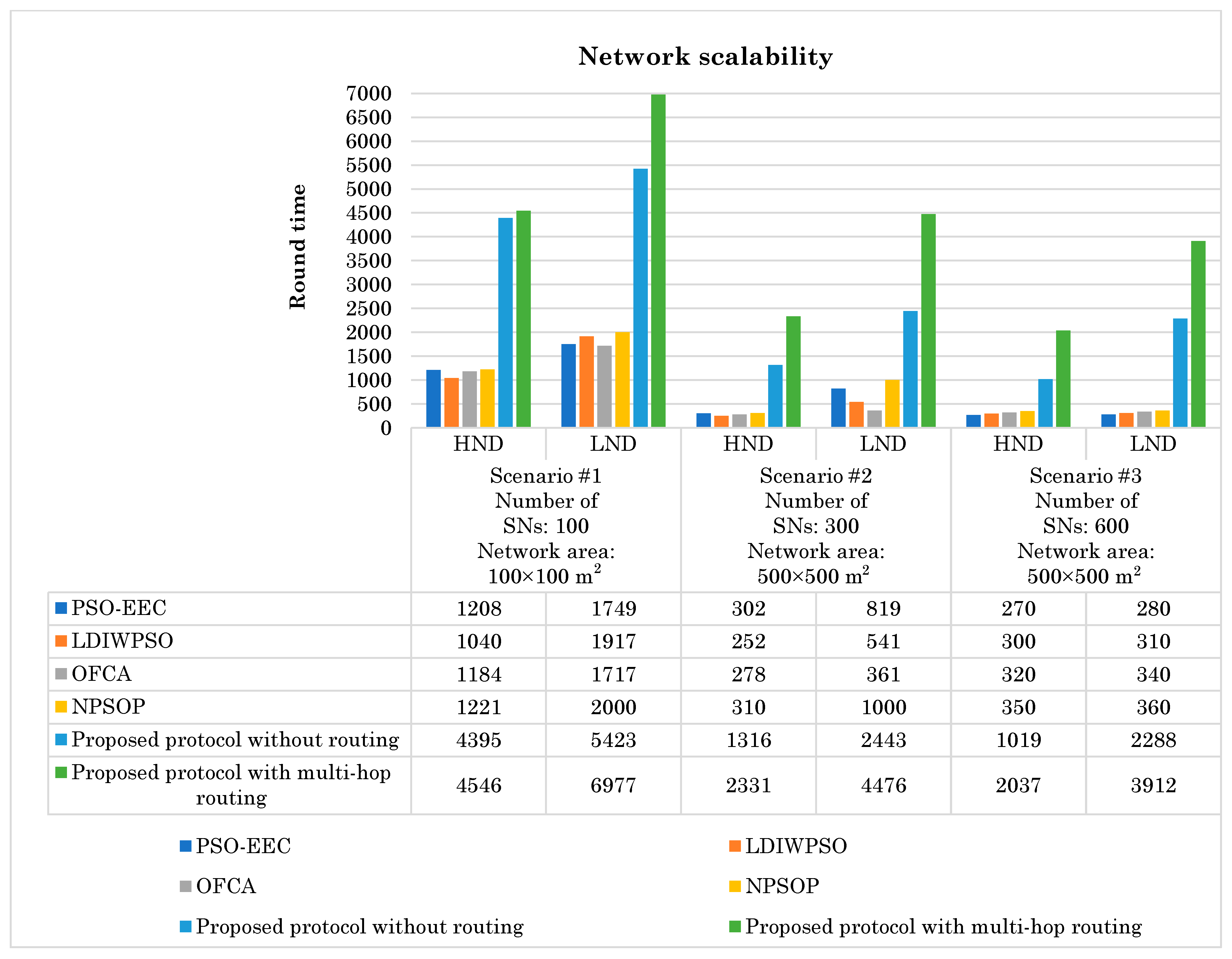
Network Lifetime: The number of rounds until the last SN runs out of energy and ceases to operate is what defines it. Two criteria were used to evaluate network lifespan: Half Node to Die (HND), which is a measure that calculates how many rounds pass from the IoT network’s initial deployment to the point at which 50% of SNs run out of energy and stop working. The term Last Node to Die (LND) refers to the total number of rounds needed for all SNs in the network to run out of energy and eventually die. The count of living and dead SNs is used to measure it.

ii.

Total Energy Consumption: This determines how much SNs consume energy after each round. The unit of measurement is Joules.

iii.

Throughput: This measures the efficiency of the network by counting the total number of data packets, in bits, that are successfully delivered to the sink node when reaching LND. Expressed in bits per second (bps), throughput indicates the network’s capacity to handle data traffic effectively, with higher throughput values reflecting more efficient data transmission.

iv.

Average Delay: This metric captures the journey time each data packet endures on its way to the sink node, measured in milliseconds (ms). It represents the typical wait time per packet as it navigates the network, reflecting the efficiency of the data flow. By calculating this delay over multiple rounds and averaging the results, we gain insight into the mean time it takes for a packet to successfully reach its destination.

6.3. Simulation Scenarios and Results

This subsection of the research paper discusses and evaluates the simulation results. We analyze the behavior of various protocols, including LDIWPSOC [40], PSO-EEC [39], OFCA [41], NPSOP [42], and our proposed protocol, both without routing and with multiple hops. Considering the parameters listed in Table 9, two scenarios are examined for the simulation. Specifically, we deployed 100 SNs within a 100 × 100 m² area and 300 SNs within a 500 × 500 m² area. In both scenarios, 10% and 5% of the total SNs are used as the number of DFGs, the same as the comparable protocols. However, our protocol has a dynamic number of DFGs. A comparison is performed using three performance metrics: network lifespan, energy consumption, and throughput assessments.

6.3.1. Simulation Scenario 1: Alive Nodes Versus Diversity of Network Sizes (Network Scalability) Evaluation

Network scalability is crucial in IoT networks, which are widely used for extensive monitoring and data collection across various applications. Data fusion grouping and routing protocols with strong scalability can effectively manage network growth and changes while maintaining performance, energy efficiency, and data transmission quality. In this study, we examine how network size affects the network lifetime of our proposed protocol. We consider various network sizes, i.e., 100 × 100 m² and 500 × 500 m², and with different network densities, i.e., 100, 300, and 600 nodes. Figure 10 illustrates how network lifetime varies with HND and LND across different IoT network sizes and node densities. The comparison includes LDIWPSOC, PSO-EEC, OFCA, NPSOP, our proposed protocol without routing, and our proposed protocol with multi-hop routing. As illustrated in Figure 10, the network lifetime decreases as the network size increases. This result is expected, as larger network sizes lead to greater communication distances between SNs and their PDFHs, as well as between PDFHs and the sink node. Consequently, the network’s energy is depleted more quickly. All the protocols fall short when compared to the proposed protocol. This difference can be attributed to the exceptional contributions of our proposed protocol, beginning with dividing the network into a dynamic number of hexagonal DFGs, which offers several benefits, particularly in enhancing the efficiency and coverage of the network area. Unlike traditional square or rectangular grids, hexagonal data fusion grouping allows for more uniform coverage with fewer overlaps or gaps, thanks to the geometric properties of hexagons. This layout is advantageous as it reduces interference between SNs, as each one in the DFG is equidistant from its neighbors, optimizing the transmission range and minimizing signal loss. Furthermore, hexagonal data fusion grouping can facilitate energy savings, as SNs in the DFG can more effectively manage resources and coordinate communication, leading to improved network longevity. This arrangement is especially favorable in large-scale IoT deployments, such as smart cities, where efficient data transmission, energy conservation, and reliable connectivity are critical. Another contribution is the strengths of the MPA used in the proposed protocol. It excels at balancing exploration and exploitation, effectively navigating the PDFH selection problem. It also has a strong ability to escape local optima, a challenge for many traditional optimization methods, as mentioned in Table 2. Its adaptability is especially useful in the PDFH selection process, where it evaluates key factors to choose the best PDFHs. By prioritizing high-energy SNs and avoiding low-energy SNs, the method helps to prevent premature failures and ensures a more balanced network load. The proposed protocol reduces energy consumption during network message exchange by integrating the data fusion grouping and routing phases. Additionally, energy consumption is optimized in both data fusion grouping and routing phases, giving the proposed protocol better scalability compared to other protocols. Beyond the proposed protocol’s application in optimizing energy dissipation and communication efficiency, the data fusion grouping approach can also address issues related to network impairments including building occlusion, device/link failures, and data redundancy. These factors are crucial for ensuring the stability and reliability of network operations.

Table 10. Improvement ratios in network lifetime for the proposed protocol without routing compared to counterparts across different network sizes.

Scenarios	Metric	PSO-EEC	LDIWPSO	OFCA	NPSOP
Scenario #1: Number of SNs: 100 Network area: 100 × 100 m2	HND	264%	323%	271%	260%
	LND	210%	183%	216%	171%
Scenario #2: Number of SNs: 300 Network area: 500 × 500 m2	HND	336%	422%	373%	325%
	LND	198%	352%	577%	144%
Scenario #3: Number of SNs: 600 Network area: 500 × 500 m2	HND	277%	240%	218%	191%
	LND	717%	638%	573%	536%

and

Table 11. Improvement ratios in the network lifetime for the proposed protocol with multi-hop routing compared to counterparts across different network sizes.

Scenarios	Metric	PSO-EEC	LDIWPSO	OFCA	NPSOP	Proposed Protocol Without Routing
Scenario #1: Number of SNs: 100 Network area: 100 × 100 m2	HND	276%	337%	284%	272%	3%
	LND	299%	264%	306%	249%	29%
Scenario #2: Number of SNs: 300 Network area: 500 × 500 m2	HND	672%	825%	738%	652%	77%
	LND	447%	727%	1140%	348%	83%
Scenario #3: Number of SNs: 600 Network area: 500 × 500 m2	HND	654%	579%	537%	482%	100%
	LND	1297%	1162%	1051%	987%	71%

present a comparison of the improvement ratios of the proposed protocol with or without multi-hop routing, respectively, in terms of network lifespan across different network sizes, to further corroborate our results. These are contrasted against the corresponding protocols in each case.

6.3.2. Simulation Scenario 2: Alive Nodes Evaluation

This scenario uses the HND and LND metrics pertaining to the number of SNs that are still active to conduct a detailed investigation of the network lifespan. Furthermore, Figure 11 clearly displays the examination’s results by contrasting the performance of our proposed protocol, that is, without routing and with multi-hop routing, with that of the LDIWPSOC, PSO-EEC, OFCA, and NPSOP protocols. Figure 11 illustrates a common and steady trend: The number of alive SNs for all protocols decreases as the number of rounds rises. This pattern is rather expected because as the number of rounds rises, the SNs’ energy consumption increases as a result of the exchange of messages and lengthy communication distances, drawing the network closer to its endpoint. The outstanding results achieved by the proposed protocol can be attributed to several key amendments. The first of these is the selection of an optimal number of PDFHs as the network demands rather than a fixed number of PDFHs. This efficiency stems largely from the fact that most message exchanges occur within the Friis free space channel propagation model. Second, the proposed protocol includes an efficient technique for selecting PDFHs, FSDFHs, and SSDFHs, utilizing the MPA. The protocol does this by, interestingly, not only choosing the right optimization method (MPA), but by also incorporating five crucial RMs in its DFFF, which made a powerful impact, taking the results to a whole new level. It is worth noting that ASBO is an innovative RM that we pioneered, specifically designed to reflect real-world conditions where obstacles interfere with wireless signals. This groundbreaking approach brings us closer to the complexities of everyday applications by factoring in the impact of obstructions on signal transmission. Additionally, unlike the methods used in directly connected protocols, the proposed protocol significantly reduces setup overhead by employing batch-round data fusion grouping. This means that data fusion grouping does not occur every round but rather in batches, and only when the energy of PDFH drops below the threshold energy, which is the average energy of DFGMs. The sink node efficiently manages this responsibility, ensuring an equal distribution of energy depletion among SNs. This significant reduction in control overhead greatly contributes to extending the IoT network’s lifetime. Additionally, after selecting PDFHs, the sink node sends a TDMA schedule through an informative message table. This message is sent only once, which minimizes the number of message exchanges between the sink node, PDFHs, and DFGMs, thereby reducing energy consumption and further prolonging the network’s lifetime. Remarkably, the proposed protocol with multi-hop routing boasts a significantly extended network lifetime, surpassing other protocols. This success is attributed to its use of multi-hop routing, where data are sent to PRs instead of directly to the sink node, regardless of the distance between PDFHs and the sink node (single-hop communication). PRs are carefully selected based on an innovative RDFCF, which has significant factors, including the distance to the sink node, CPRs’ RE, and ASBO. Consequently, the advantages of our proposed concepts are clearly evident, demonstrating superior performance compared to other protocols. Notably, the HND and LND values in the proposed protocol are significantly higher than those in other protocols across various network sizes. To assess the effectiveness of the proposed protocol compared to other protocols,

Table 12. Comparative analysis of improvement ratios: HND and LND in the proposed protocol versus counterparts.

Items	Protocols Considred in Comparision	HND	Improvement Ratios for the Proposed Protocol Without Routing	Improvement Ratios for the Proposed Protocol with Multi-Hop Routing	LND	Improvement Ratio for the Proposed Protocol Without Routing	Improvement Ratio for the Proposed Protocol with Multi-Hop Routing
Scenario #1 Number of SNs: 100 Number of DFHs: 10% Network area: 100 × 100 m2	PSO-EEC	1310	235%	314%	1933	135%	261%
	LDIWPSO	1288	241%	321%	1352	236%	416%
	OFCA	1415	211%	283%	1776	156%	293%
	NPSOP	1465	200%	270%	2078	119%	236%
	Proposed protocol without routing	4395	NA	23%	4546	NA	53%
	Proposed protocol with multi-hop routing	5423	NA	NA	6977	NA	NA
Scenario #1 Number of SNs: 100 Number of DFHs: 5% Network area: 100 × 100 m2	PSO-EEC	1208	264%	349%	1749	160%	299%
	LDIWPSO	1040	323%	421%	1917	137%	264%
	OFCA	1184	271%	358%	1717	165%	306%
	NPSOP	1221	260%	344%	2000	127%	249%
	Proposed protocol without routing	4395	NA	23%	4546	NA	53%
	Proposed protocol with multi-hop routing	5423	NA	NA	6977	NA	NA
Scenario #2 Number of SNs: 300 Number of DFHs: 10% Network area: 500 × 500 m2	PSO-EEC	256	414%	811%	396	517%	1030%
	LDIWPSO	277	375%	742%	380	543%	1078%
	OFCA	307	329%	659%	367	566%	1120%
	NPSOP	318	314%	633%	397	515%	1027%
	Proposed protocol without routing	1316	NA	77%	2443	NA	83%
	Proposed protocol with multi-hop routing	2331	NA	NA	4476	NA	NA
Scenario #2 Number of SNs: 300 Number of DFHs: 5% Network area: 500 × 500 m2	PSO-EEC	302	336%	672%	819	198%	447%
	LDIWPSO	252	422%	825%	541	352%	727%
	OFCA	278	373%	738%	361	577%	1140%
	NPSOP	310	325%	652%	1000	144%	348%
	Proposed protocol without routing	1316	NA	77%	2443	NA	83%
	Proposed protocol with multi-hop routing	2331	NA	NA	4476	NA	NA

NA: means not available, as the protocol is compared with itself, which is not meaningful.

presents the improvement ratios across HND and LND scenarios.

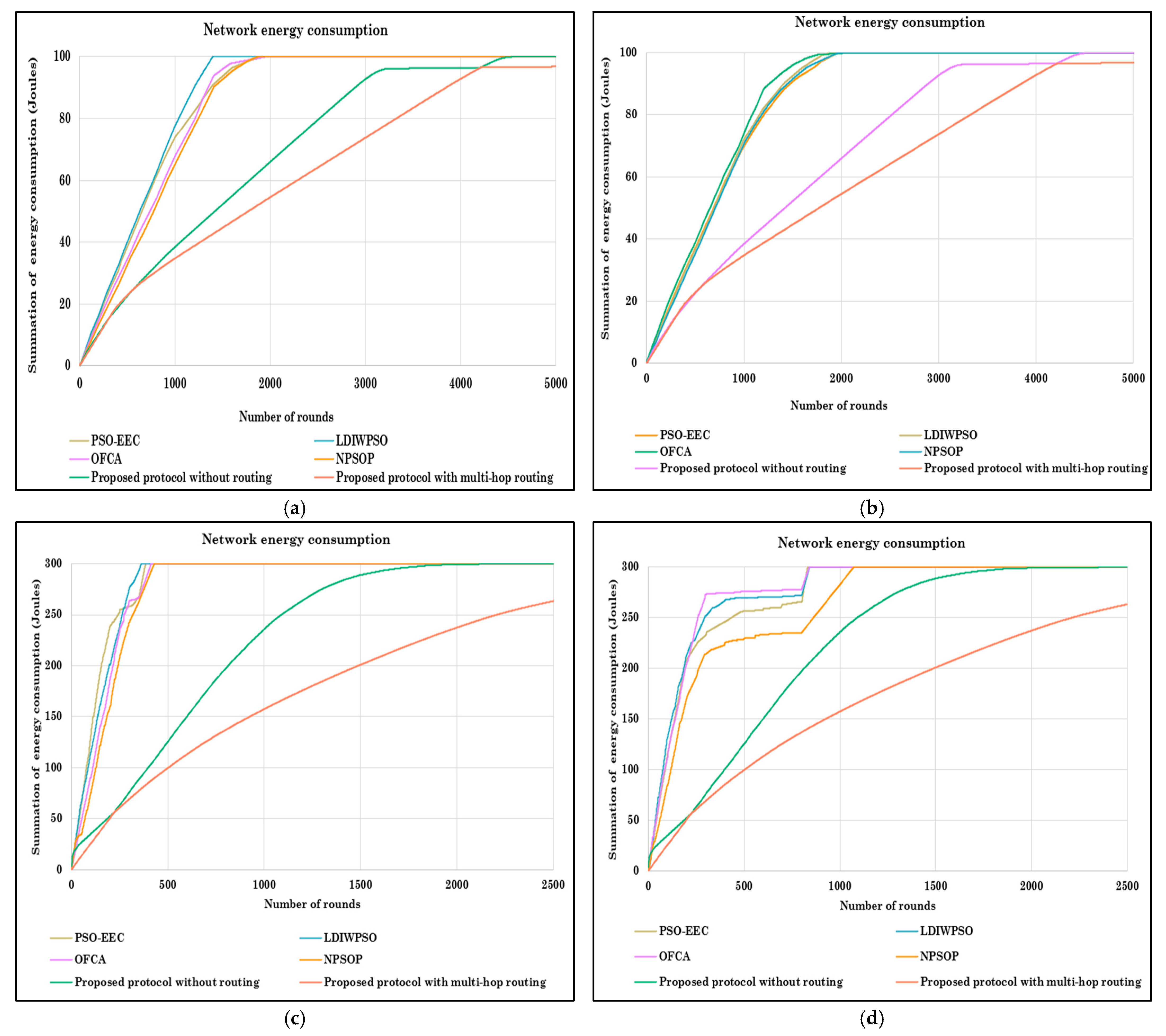
6.3.3. Simulation Scenario 3: Energy Consumption Evaluation

In this subsection, we dive into the simulation results that reveal how energy consumption varies across different protocols. Specifically, we compare the total energy consumption of our cutting-edge protocol with its counterparts: LDIWPSOC, PSO-EEC, OFCA, and NPSOP. As shown in Figure 12, it is clear that energy consumption rises as data transmission and distances increase. While these other protocols have made strides, they still fall short of what our proposed protocol offers, both with and without routing options, and especially when using multi-hop routing. Our protocol goes above and beyond to minimize energy consumption by integrating a host of innovative features. From a novel scheduling strategy to an optimal DFG formation process that secures the ideal number of PDFHs, it is designed to maximize efficiency. One of our key contributions is regrouping after a set of rounds, triggered when a PDFH’s energy falls below the DFG’s average. This approach significantly extends the network’s lifespan by ensuring SNs with lower energy are less likely to become PDFHs, effectively conserving their resources. By tackling network impairments, our protocol delivers a noticeable boost in overall performance, truly setting a new standard for energy-efficient networking. In essence, backup CHs (i.e., FSDFH, SSDFH, FSDFR, and SSDFRs) play a crucial role in maintaining the stability, reliability, and efficiency of data transmission. These backups are responsible for aggregating data from SNs and relaying it to the sink node or other PRs. However, IoT networks are often prone to SN failures due to battery depletion, connectivity issues, or environmental factors, which can disrupt communication and data flow. Implementing backup CHs provides a fail-safe mechanism that ensures continuous network operation, even when PDFHs fail. FSDFH and SSDFH can immediately take over data aggregation and forwarding tasks, minimizing data loss, reducing downtime, and maintaining network performance. This redundancy is essential for critical applications, such as healthcare monitoring or industrial automation, where consistent data transmission is vital for decision-making and operational efficiency. More to the point, the routing strategy in the proposed protocol with multi-hop routing, which is based on a novel RDFCF, helps to reduce the communication distances between SNs and the sink node, which reduces energy consumption and enhances load balancing for PDFHs that are located farther away from the sink node.

Table 13. Comparative analysis of improvement ratios: energy consumption in the proposed protocol versus counterparts.

Items	Protocols Considred in Comparision	Improvement Ratio for the Proposed Protocol Without Routing	Improvement Ratio for the Proposed Protocol with Multi-Hop Routing
Scenario #1 Number of SNs: 100 Number of CHs: 10% Network area: 100 × 100 m2	PSO-EEC	135%	260%
	LDIWPSO	225%	399%
	OFCA	133%	258%
	NPSOP	143%	273%
	Proposed protocol without routing	NA	53%
	Proposed protocol with multi-hop routing	NA	NA
Scenario #1 Number of SNs: 100 Number of CHs: 5% Network area: 100 × 100 m2	PSO-EEC	131%	254%
	LDIWPSO	137%	264%
	OFCA	126%	247%
	NPSOP	130%	253%
	Proposed protocol without routing	NA	53%
	Proposed protocol with multi-hop routing	NA	NA
Scenario #2 Number of SNs: 300 Number of CHs: 5% Network area: 500 × 500 m2	PSO-EEC	194%	438%
	LDIWPSO	190%	432%
	OFCA	190%	432%
	NPSOP	128%	317%
	Proposed protocol without routing	NA	83%
	Proposed protocol with multi-hop routing	NA	NA
Scenario #2 Number of SNs: 300 Number of CHs: 10% Network area: 500 × 500 m2	PSO-EEC	534%	1063%
	LDIWPSO	573%	1133%
	OFCA	490%	981%
	NPSOP	468%	941%
	Proposed protocol without routing	NA	83%
	Proposed protocol with multi-hop routing	NA	NA

NA: means not available, as the protocol is compared with itself, which is not meaningful.

displays the improvement ratios over a range of total rounds to evaluate the proposed protocol’s potency compared to other protocols.

6.3.4. Simulation Scenario 4: Throughput Evaluation

In this context, the contributions of our proposed protocol, both without routing and with multi-hop routing, have been verified with respect to throughput when reaching LND. Figure 13 shows the throughput of the network until round n for the proposed protocol and its counterparts. The results show that in all protocols, larger network area sizes result in lower throughput. Furthermore, our proposed protocol performs substantially better than the other protocols for all network sizes due to the innovative ideas that were previously described. It goes without saying that the proposed protocol not only doubles the network’s lifespan but also enhances data transmission rates and energy efficiency. The proposed protocol sustains network functionality for a far longer period of time than previous ones. This results in more data being sent to the sink node, thereby increasing the overall network throughput. A pertinent question that may arise is the extent to which the proposed protocol outperforms other protocols. Complementing this graphical analysis,

Table 14. Comparative analysis of improvement ratios: throughput in the proposed protocol versus counterparts.

Items	Protocols Considred in Comparision	Throughput (×108)	Improvement Ratio for the Proposed Protocol Without Routing	Improvement Ratio for the Proposed Protocol with Multi-Hop Routing
Scenario #1 Number of SNs: 100 Number of DFHs: 10% Network area: 100 × 100 m2	PSO-EEC	4.3543	51%	66%
	LDIWPSO	4.5695	44%	58%
	OFCA	4.8841	35%	48%
	NPSOP	4.9338	33%	47%
	Proposed protocol without routing	6.5752	NA	10%
	Proposed protocol with multi-hop routing	7.2344	NA	NA
Scenario #1 Number of SNs: 100 Number of DFHs: 5% Network area: 100 × 100 m2	PSO-EEC	4.3295	52%	67%
	LDIWPSO	4.5530	44%	59%
	OFCA	4.7434	39%	53%
	NPSOP	4.8179	36%	50%
	Proposed protocol without routing	6.5752	NA	10%
	Proposed protocol with multi-hop routing	7.2344	NA	NA
Scenario #2 Number of SNs: 300 Number of DFHs: 10% Network area: 300 × 300 m2	PSO-EEC	2.8610	89%	101%
	LDIWPSO	3.5661	51%	61%
	OFCA	3.4373	57%	67%
	NPSOP	3.8712	40%	48%
	Proposed protocol without routing	5.4008	NA	6%
	Proposed protocol with multi-hop routing	5.7432	NA	NA
Scenario #2 Number of SNs: 300 Number of DFHs: 5% Network area: 300 × 300 m2	PSO-EEC	2.5288	114%	127%
	LDIWPSO	3.1322	72%	83%
	OFCA	2.4949	116%	130%
	NPSOP	3.2475	66%	77%
	Proposed protocol without routing	5.4008	NA	6%
	Proposed protocol with multi-hop routing	5.7432	NA	NA

NA: means not available, as the protocol is compared with itself, which is not meaningful.

quantifies the improvement ratios of the throughput, offering a precise evaluation of the proposed protocol’s efficiency and dominance over alternative approaches.

6.3.5. Simulation Scenario 5: Average Delay Evaluation

Figure 14 presents an in-depth comparative analysis of the average delay observed in the proposed protocol versus existing protocols. The results unequivocally demonstrate that the proposed protocol, whether employed with or without multi-hop routing, delivers superior performance, achieving the lowest average delay across the board. This remarkable enhancement stems from the sophisticated and adaptive algorithms embedded within the proposed protocol, as discussed earlier, enabling it to outperform its counterparts by a significant margin. This metric collectively underscores the protocol’s ability to redefine delay performance benchmarks in IoT networks, solidifying its utility in latency-critical applications.

6.4. Analysis of Underlying Causes and Correlations of Results

The proposed protocol outperforms others in network lifespan, energy consumption, throughput, and delay due to its strategic design. The use of a hexagonal DFG ensures uniform coverage and minimal signal loss, which conserves energy and extends network lifetime. The MPA and dynamic RMs optimize PDFH selection, balancing load and preventing node failures. Multi-hop routing reduces communication distance, conserving energy, while the RDFCF mechanism selects optimal relay nodes to minimize energy usage. Data fusion grouping reduces control overhead, and backup mechanisms maintain data flow during node failures. These factors collectively enhance throughput, minimize delay, and optimize energy usage, especially for latency-sensitive IoT applications.

The correlation between network lifespan, energy consumption, throughput, and average delay reveals several important correlations as follows:

• Network lifespan and energy consumption: There is an inverse correlation between energy consumption and network lifespan. Protocols that minimize energy usage extend the operational time of SNs, thereby prolonging the overall network lifespan. The proposed protocol achieves this by optimizing routing and PDFH selection, reducing unnecessary energy expenditure.
• Network lifespan and throughput: A longer network lifespan directly contributes to higher throughput, as the network remains functional for a more extended period of time, allowing more data packets to be transmitted to the sink node. This correlation is evident in the proposed protocol, where efficient energy management ensures sustained data transmission over time.
• Energy consumption and average delay: Lower energy consumption correlates with reduced average delay. Efficient energy usage ensures that SNs and PDFHs remain operational and responsive, minimizing the time required for data transmission. The proposed protocol’s optimized scheduling and routing strategies contribute to this correlation by enhancing both energy efficiency and transmission speed.
• Throughput and average delay: While high throughput generally indicates efficient data transmission, it can sometimes lead to increased network congestion and higher delays. However, the proposed protocol balances this by employing multi-hop routing and adaptive scheduling, which maintain high throughput without significantly increasing delay.

7. Conclusions, Home Recommendations, and Future Directions

The majority of IoT SNs utilized in smart city applications have limited battery life and are not rechargeable. This characteristic makes IoT networks highly vulnerable to sudden spikes in energy consumption, emphasizing the critical need for energy conservation to ensure prolonged network operation. Addressing this challenge, our work proposes a novel IoT routing protocol incorporating innovative energy-efficient data fusion grouping and routing algorithms. At the core of this protocol is the data fusion grouping algorithm, which plays a pivotal role in enhancing energy efficiency by uniformly dividing the network sensing area into hexagonal DFGs. This not only minimizes redundant data transmission but also balances energy consumption across the network, thereby extending the operational lifespan of the proposed protocol. Each SN responds with an information message containing its ID, location, and RE when the sink node sends a request information message. Using the DFG algorithm, the sensing area is structured systematically, while the MPA is employed to determine the PDFH, FSDFH, and SSDFH. Five critical RMs—the SN’s RE, average distance between DFGMs, distance from the sink node, ASBO, and the ratio of the average rounds all the DFGMs served as PDFHs to the rounds served by the CDFH_i—were incorporated to optimize routing and resource allocation. Further, we developed a new TDMA scheme, a novel RDFCF, and an innovative DFFF. The comprehensive simulation results demonstrate the superior performance of the proposed protocol, particularly in terms of network lifetime, total remaining energy, throughput, and average delay over several rounds, both with and without multi-hop routing. Comparative analyses against relevant protocols, including LDIWPSOC, PSO-EEC, OFCA, and NPSOP, confirm the significant improvements achieved due to the enhancements introduced in our approach. Moreover, our work addresses critical real-world challenges such as building occlusions at various heights, device/link failures, and data redundancy obstacles. These considerations place our protocol ahead of its competitors, particularly in challenging environmental settings. The robust data fusion algorithm incorporated in our protocol not only optimizes data transmission efficiency but also effectively mitigates data redundancy, making it a cornerstone of the protocol’s success in extending network longevity and reliability. By addressing these critical aspects comprehensively, our proposed protocol establishes a strong foundation for energy-efficient and reliable IoT networks in smart city applications. Therefore, we enthusiastically urge the Greater Amman Municipality (GAM) and the Information and Communication Technology (ICT) industry to take the adoption of these models into consideration and implement them in reality, given the remarkable outcomes attained with the smart models that have been presented. This advice is especially important as the ICT industry and GAM have not yet proposed or implemented any smart model projects for Amman, the capital of Jordan. Future research could focus on further enhancing the PDFH selection and routing mechanisms in IoT networks for smart cities. One promising direction is to incorporate machine learning techniques, which could enable predictive analytics to anticipate energy spikes and optimize routing paths preemptively. Another avenue for improvement is to test the protocol’s effectiveness in larger-scale smart city environments with more diverse obstacles and real-time data requirements, which would provide insights into its scalability and robustness.

References

1. Darabkh, K.A.; Al-Akhras, M.; Khalifeh, A.F.; Jafar, I.F.; Jubair, F. An innovative RPL objective function for broad range of IoT domains utilizing fuzzy logic and multiple metrics. Expert Syst. Appl. 2022, 205, 117593. [Google Scholar] [CrossRef]
2. Vishwakarma, A.K.; Chaurasia, S.; Kumar, K.; Singh, Y.N.; Chaurasia, R. Internet of things technology, research, and challenges: A survey. Multimed. Tools Appl. 2024, 1–36. [Google Scholar] [CrossRef]
3. Zeng, F.; Pang, C.; Tang, H. Sensors on Internet of Things Systems for the Sustainable Development of Smart Cities: A Systematic Literature Review. Sensors 2024, 24, 2074. [Google Scholar] [CrossRef]
4. Zhang, Z.; Zhang, Y.; Tian, H.; Martin, A.; Liu, Z.; Ding, W. A survey of evidential clustering: Definitions, methods, and applications. Inf. Fusion 2025, 115, 102736. [Google Scholar]
5. Liu, Z.; Li, J.; Zhang, X.; Wang, X. Multi-level information fusion for missing multi-label learning based on stochastic concept clustering. Inf. Fusion 2024, 115, 102775. [Google Scholar] [CrossRef]
6. Yu, B.; Xu, R.; Cai, M.; Ding, W. A clustering method based on multi-positive–negative granularity and attenuation-diffusion pattern. Inf. Fusion 2023, 103, 102137. [Google Scholar] [CrossRef]
7. Xie, J.; Jiang, L.; Xia, S.; Xiang, X.; Wang, G. An adaptive density clustering approach with multi-granularity fusion. Inf. Fusion 2024, 106, 102273. [Google Scholar] [CrossRef]
8. Darabkh, K.A.; Al-Akhras, M.; Zomot, J.N.; Atiquzzaman, M. RPL Routing Protocol over IoT: A Comprehensive Survey, Recent Advances, Insights, Bibliometric Analysis, Recommendations, and Future Directions. J. Netw. Comput. Appl. 2022, 207, 103476. [Google Scholar]
9. Zaman, M.; Puryear, N.; Abdelwahed, S.; Zohrabi, N. A Review of IoT-Based Smart City Development and Management. Smart Cities 2024, 7, 1462–1501. [Google Scholar] [CrossRef]
10. Samiayya, D.; Radhika, S.; Chandrasekar, A. An optimal model for enhancing network lifetime and cluster head selection using hybrid snake whale optimization. Peer Peer Netw. Appl. 2023, 16, 1959–1974. [Google Scholar] [CrossRef]
11. Hosseinzadeh, M.; Hemmati, A.; Rahmani, A.M. Clustering for smart cities in the internet of things: A review. Clust. Comput. 2022, 25, 4097–4127. [Google Scholar] [CrossRef]
12. Wang, Z.; Duan, J.; Xing, P. Multi-Hop Clustering and Routing Protocol Based on Enhanced Snake Optimizer and Golden Jackal Optimization in WSNs. Sensors 2024, 24, 1348. [Google Scholar] [CrossRef] [PubMed]
13. Darabkh, K.A.; AlAdwan, H.H.; Al-Akhras, M.; Jubair, F.; Rahamneh, S. A revolutionary RPL-based IoT routing protocol for monitoring building structural health in smart city domain utilizing equilibrium optimizer algorithm. Soft Comput. 2024, 28, 10099–10138. [Google Scholar] [CrossRef]
14. Chen, Y.; Liu, X.; Rao, M.; Qin, Y.; Wang, Z.; Ji, Y. Explicit speed-integrated LSTM network for non-stationary gearbox vibration representation and fault detection under varying speed conditions. Reliab. Eng. Syst. Saf. 2024, 254, 110596. [Google Scholar] [CrossRef]
15. Darabkh, K.A.; Al-Akhras, M. The Potential of Computational Intelligence to Extend the Lifespan of Internet of Things Power-Limited Sensor Networks. In Proceedings of the 2024 International Conference on Software, Telecommunications and Computer Networks (SoftCOM), Split, Croatia, 26–28 September 2024; pp. 1–6. [Google Scholar]
16. Ramalingam, S.; Dhanasekaran, S.; Sinnasamy, S.S.; Salau, A.O.; Alagarsamy, M. Performance enhancement of efficient clustering and routing protocol for wireless sensor networks using improved elephant herd optimization algorithm. Wirel. Netw. 2024, 30, 1773–1789. [Google Scholar] [CrossRef]
17. Chai, X.; Lee, B.G.; Hu, C.; Pike, M.; Chieng, D.; Wu, R.; Chung, W.Y. IoT-FAR: A multi-sensor fusion approach for IoT-based firefighting activity recognition. Inf. Fusion 2025, 113, 102650. [Google Scholar]
18. Huang, C.; Coskun, S.; Karimi, H.R.; Ding, W. A distributed state and fault estimation scheme for state-saturated systems with quantized measurements over sensor networks. Inf. Fusion 2024, 110, 102452. [Google Scholar] [CrossRef]
19. Ji, Y.; Huang, Y.; Zeng, J.; Ren, L.; Chen, Y. A physical–data-driven combined strategy for load identification of tire type rail transit vehicle. Reliab. Eng. Syst. Saf. 2024, 253, 110493. [Google Scholar] [CrossRef]
20. Kaleybar, H.J.; Davoodi, M.; Brenna, M.; Zaninelli, D. Applications of Genetic Algorithm and Its Variants in Rail Vehicle Systems: A Bibliometric Analysis and Comprehensive Review. IEEE Access 2023, 11, 68972–68993. [Google Scholar] [CrossRef]
21. Kumaravel, V.; Panneerselvam, A. A multi objective Tabu particle swarm optimization for effective cluster head selection in WSN. Clust. Comput. 2019, 22, 12275–12282. [Google Scholar]
22. Bharathi, M.; Srinivas, T.A.S. Exploring Ant Colony Optimization for Enhanced Routing in IoT Networks: A Survey. Adv. Image Process. Pattern Recognit. 2024, 7, 68–83. [Google Scholar]
23. Płaczek, B. Prediction-based data reduction with dynamic target node selection in IoT sensor networks. Futur. Gener. Comput. Syst. 2023, 152, 225–238. [Google Scholar] [CrossRef]
24. Darabkh, K.A.; AlAdwan, H.H.; Al-Akhras, M.; Jubair, F.; Rahamneh, S. A New Routing Protocol for Low-Power and Lossy Networks Utilizing Computational Intelligence over IoT Networks. In Proceedings of the 2023 IEEE Global Conference on Artificial Intelligence and Internet of Things (GCAIoT), Dubai, United Arab Emirates, 10–11 December 2023; pp. 97–102. [Google Scholar]
25. Darabkh, K.A.; Asma’a, B.A.; Al-Akhras, M.; Wafa’a, K.K. Improving Network Lifetime in IoT Sensor Network Based on Particle Swarm Optimization, Clustering, and Mobile Sink. In Proceedings of the 2022 4th IEEE Middle East and North Africa COMMunications Conference (MENACOMM), Amman, Jordan, 6–8 December 2022. [Google Scholar]
26. Amutha, J.; Sharma, S.; Sharma, S.K. An energy efficient cluster based hybrid optimization algorithm with static sink and mobile sink node for Wireless Sensor Networks. Expert Syst. Appl. 2022, 203, 117334. [Google Scholar]
27. Suresh, S.S.; Prabhu, V.; Parthasarathy, V.; Senthilkumar, G.; Gundu, V. Intelligent data routing strategy based on federated deep reinforcement learning for IOT-enabled wireless sensor networks. Meas. Sens. 2024, 31, 101012. [Google Scholar] [CrossRef]
28. Priyadarshi, R. Energy-Efficient Routing in Wireless Sensor Networks: A Meta-heuristic and Artificial Intelligence-based Approach: A Comprehensive Review. Arch. Comput. Methods Eng. 2024, 31, 2109–2137. [Google Scholar] [CrossRef]
29. Gao, J.; Wang, Z.; Lei, Z.; Wang, R.-L.; Wu, Z.; Gao, S. Feature selection with clustering probabilistic particle swarm optimization. Int. J. Mach. Learn. Cybern. 2024, 15, 3599–3617. [Google Scholar] [CrossRef]
30. Ravi, G.; Das, M.S.; Karmakonda, K. Reliable cluster based data aggregation scheme for IoT network using hybrid deep learning techniques. Meas. Sens. 2023, 27, 100744. [Google Scholar] [CrossRef]
31. Darabkh, K.A.; Al-Akhras, M. An Improved Routing Protocol for IoT Sensors Utilizing Clustering Techniques and Optimization Methods. In Proceedings of the 6th IEEE International Conference on Advanced Communication Technologies and Networking (IEEE CommNet 2023), Rabat, Morocco, 11–13 December 2023. [Google Scholar]
32. Darabkh, K.A.; Zomot, J.N.; Al-qudah, Z. EDB-CHS-BOF: Energy and Distance Based Cluster Head Selection with Balanced Objective Function Protocol. IET Commun. 2019, 13, 3168–3180. [Google Scholar]
33. Heidari, E. A novel energy-aware method for clustering and routing in IoT based on whale optimization algorithm & Harris Hawks optimization. Computing 2024, 106, 1013–1045. [Google Scholar] [CrossRef]
34. He, S.; Li, Q.; Khishe, M.; Mohammed, A.S.; Mohammadi, H.; Mohammadi, M. The optimization of nodes clustering and multi-hop routing protocol using hierarchical chimp optimization for sustainable energy efficient underwater wireless sensor networks. Wirel. Netw. 2023, 30, 233–252. [Google Scholar] [CrossRef]
35. Darabkh, K.A.; Amareen, A.B.; Al-Akhras, M.; Kassab, W.K. An innovative cluster-based power-aware protocol for Internet of Things sensors utilizing mobile sink and particle swarm optimization. Neural Comput. Appl. 2023, 35, 19365–19408. [Google Scholar] [CrossRef]
36. Somula, R.; Cho, Y.; Mohanta, B.K. SWARAM: Osprey Optimization Algorithm-Based Energy-Efficient Cluster Head Selection for Wireless Sensor Network-Based Internet of Things. Sensors 2024, 24, 521. [Google Scholar] [CrossRef]
37. Bian, Z.; Qu, J.; Zhou, J.; Jiang, Z.; Wang, S. Weighted adaptively ensemble clustering method based on fuzzy Co-association matrix. Inf. Fusion 2023, 103, 102099. [Google Scholar] [CrossRef]
38. Zhou, X.; Yang, Q.; Liu, Q.; Liang, W.; Wang, K.; Liu, Z.; Ma, J.; Jin, Q. Spatial–Temporal Federated Transfer Learning with multi-sensor data fusion for cooperative positioning. Inf. Fusion 2023, 105, 102182. [Google Scholar] [CrossRef]
39. Rawat, P.; Chauhan, S. Particle swarm optimization-based energy efficient clustering protocol in wireless sensor network. Neural Comput. Appl. 2021, 33, 14147–14165. [Google Scholar] [CrossRef]
40. Choudhary, S.; Sugumaran, S.; Belazi, A.; El-Latif, A.A.A. Linearly decreasing inertia weight PSO and improved weight factor-based clustering algorithm for wireless sensor networks. J. Ambient. Intell. Humaniz. Comput. 2023, 14, 6661–6679. [Google Scholar] [CrossRef]
41. Giri, A.; Dutta, S.; Neogy, S. An Optimized Fuzzy Clustering Algorithm for Wireless Sensor Networks. Wirel. Pers. Commun. 2022, 126, 2731–2751. [Google Scholar] [CrossRef]
42. Huangshui, H.; Xinji, F.; Chuhang, W.; Ke, L.; Yuxin, G. A Novel Particle Swarm Optimization-Based Clustering and Routing Protocol for Wireless Sensor Networks. Wirel. Pers. Commun. 2023, 133, 2175–2202. [Google Scholar] [CrossRef]
43. Faramarzi, A.; Heidarinejad, M.; Mirjalili, S.; Gandomi, A.H. Marine Predators Algorithm: A nature-inspired metaheuristic. Expert Syst. Appl. 2020, 152, 113377. [Google Scholar] [CrossRef]
44. Al-Betar, M.A.; Awadallah, M.A.; Makhadmeh, S.N.; Alyasseri, Z.A.A.; Al-Naymat, G.; Mirjalili, S. Marine Predators Algorithm: A Review. Arch. Comput. Methods Eng. 2023, 30, 3405–3435. [Google Scholar] [CrossRef]
45. Rai, R.; Dhal, K.G.; Das, A.; Ray, S. An Inclusive Survey on Marine Predators Algorithm: Variants and Applications. Arch. Comput. Methods Eng. 2023, 30, 3133–3172. [Google Scholar] [PubMed]
46. Mugemanyi, S.; Qu, Z.; Rugema, F.X.; Dong, Y.; Wang, L.; Bananeza, C.; Nshimiyimana, A.; Mutabazi, E. Marine predators algorithm: A comprehensive review. Mach. Learn. Appl. 2023, 12, 100471. [Google Scholar] [CrossRef]
47. Darabkh, K.A.; Zomot, J.N.; Al-Qudah, Z.; Khalifeh, A.F. Impairments-aware time slot allocation model for energy-constrained multi-hop clustered IoT nodes considering TDMA and DSSS MAC protocols. J. Ind. Inf. Integr. 2021, 25, 100243. [Google Scholar] [CrossRef]
48. Shahzad, M.K.; Islam, S.M.R.; Kwak, K.-S.; Nkenyereye, L. AEF: Adaptive En-Route Filtering to Extend Network Lifetime in Wireless Sensor Networks. Sensors 2019, 19, 4036. [Google Scholar] [CrossRef]
49. Darabkh, K.A.; El-Yabroudi, M.Z.; El-Mousa, A.H. BPA-CRP: A balanced power-aware clustering and routing protocol for wireless sensor networks. Ad. Hoc Netw. 2018, 82, 155–171. [Google Scholar] [CrossRef]
50. Darabkh, K.A.; Al-Akhras, M. Prolonging IoT Sensor Networks Lifetime for Different Smart City Applications Utilizing a Three-dimension MPA Based Fitness Function. In Proceedings of the 2024 IEEE 15th Annual Information Technology, Electronics and Mobile Communication Conference (IEMCON 2024), Berkeley, CA, USA, 24–26 October 2024. [Google Scholar]
51. Darabkh, K.A.; Al-Akhras, M. A Five-dimension MPA Based Fitness Function for Optimizing Energy in IoT Sensor Networks Considering Various Smart City Applications. In Proceedings of the 2024 IEEE 15th Annual Information Technology, Electronics and Mobile Communication Conference (IEMCON 2024), Berkeley, CA, USA, 24–26 October 2024. [Google Scholar]
52. Dehkordi, A.B. EDBLSD-IIoT: A comprehensive hybrid architecture for enhanced data security, reduced latency, and optimized energy in industrial IoT networks. J. Supercomput. 2025, 81, 359. [Google Scholar] [CrossRef]
53. Rathee, M.; Kumar, S.; Dilip, K.; Dohare, U. Towards energy balancing optimization in wireless sensor networks: A novel quantum inspired genetic algorithm based sinks deployment approach. Ad. Hoc. Netw. 2023, 153, 103350. [Google Scholar] [CrossRef]
54. Gad, A.G. Particle Swarm Optimization Algorithm and Its Applications: A Systematic Review. Arch. Comput. Methods Eng. 2022, 29, 2531–2561. [Google Scholar]
55. Abdulzahra, A.M.K.; Al-Qurabat, A.K.M.; Abdulzahra, S.A. Optimizing energy consumption in WSN-based IoT using unequal clustering and sleep scheduling methods. Int. Things 2023, 22, 100765. [Google Scholar] [CrossRef]
56. Rui, K. Improving energy efficiency in wireless sensor networks (WSNs) using two-level fuzzy clustering and Artificial Bee Colony (ABC) optimization. Int. J. Electron. 2025, 1–26. [Google Scholar] [CrossRef]
57. Al-Betar, M.A.; Abu Doush, I.; Makhadmeh, S.N.; Al-Naymat, G.; Alomari, O.A.; Awadallah, M.A. Equilibrium optimizer: A comprehensive survey. Multimed. Tools Appl. 2023, 83, 29617–29666. [Google Scholar] [CrossRef]
58. Shen, B.; Khishe, M.; Mirjalili, S. Evolving Marine Predators Algorithm by dynamic foraging strategy for real-world engineering optimization problems. Eng. Appl. Artif. Intell. 2023, 123, 106207. [Google Scholar] [CrossRef]
59. Wang, Y.; Henning, I. A Deterministic Distributed TDMA Scheduling Algorithm for Wireless Sensor Networks. In Proceedings of the 2007 International Conference on Wireless Communications, Networking and Mobile Computing, Shanghai, China, 21–25 September 2007; pp. 2759–2762. [Google Scholar]
60. Firouz, N.; Masdari, M.; Sangar, A.B.; Majidzadeh, K. A Hybrid Multi objective Algorithm for Imbalanced Controller Placement in Software Defined Networks. J. Netw. Syst. Manag. 2022, 30, 51. [Google Scholar] [CrossRef]
Figure 1. DFG model of an IoT network area for the proposed protocol. (a) DFG model of a IoT network area for the proposed protocol without routing. (b) DFG model of a IoT network area for the proposed protocol with multi-hop routing.
Smartcities 08 00064 g001
Figure 2. Breaking down the operational lifetime of the IoT network in the proposed protocol without routing.
Smartcities 08 00064 g002
Figure 3. Breaking down the operational lifetime of the IoT network in the proposed protocol with multi-hop routing.
Smartcities 08 00064 g003
Figure 4. Partitioning the network area into equally sized hexagonal DFG.
Smartcities 08 00064 g004
Figure 5. Partitioning the network area into equally sized hexagonal DFGs. (a) A 300 × 300 m2 network area before partitioning. (b) Partitioning network area into equal-sized hexagonal DFGs. (c) Distributing SNs into the formed DFGs based on their locations.
Smartcities 08 00064 g005
Figure 6. A variety of IoT applications spanning different network areas. (a) Model for smart logistics park for 100 × 100 m2 of network area. (b) Model for smart medical center for 200 × 200 m2 of network area. (c) Model for smart factories zone for 300 × 300 m2 of network area. (d) Model for smart university for 400 × 400 m2 of network area. (e) Model for smart city for 500 × 500 m2 of network area.
Smartcities 08 00064 g006
Figure 7. The selected PDFHs utilizing the MPA for the proposed protocol.
Smartcities 08 00064 g007
Figure 8. Representation of building occlusions based on a PDFH position and the coverage area.
Smartcities 08 00064 g008
Figure 9. SNs distribution for the first and second scenarios.
Smartcities 08 00064 g009
Figure 10. Number of alive nodes vs. number of rounds: A comparison with counterpart protocols across various IoT network sizes (PSO-EEC [39], LDIWPSO [40], OFCA [41], and NPSOP [42]).
Smartcities 08 00064 g010
Figure 11. Number of alive nodes vs. number of rounds: A comparison with counterpart protocols for Scenarios 1 and 2 (PSO-EEC [39], LDIWPSO [40], OFCA [41], and NPSOP [42]). (a) Scenario #1: Network area: 100 × 100 m2 with 100 nodes, 10% DFHs. (b) Scenario #1: Network area: 100 × 100 m2 with 100 nodes, 5% DFHs. (c) Scenario #2: Network area: 500 × 500 m2 with 300 nodes, 10% DFHs. (d) Scenario #2: Network area: 500 × 500 m2 with 300 nodes, 5% DFHs.
Smartcities 08 00064 g011
Figure 12. Network energy consumption vs. number of rounds: A comparison with counterpart protocols for Scenarios 1 and 2 (PSO-EEC [39], LDIWPSO [40], OFCA [41], and NPSOP [42]). (a) Scenario #1: Network area: 100 × 100 m2 with 100 nodes, 10% DFHs. (b) Scenario #1: Network area: 100 × 100 m2 with 100 nodes, 5% DFHs. (c) Scenario #2: Network area: 500 × 500 m2 with 300 nodes, 10% DFHs. (d) Scenario #2: Network area: 500 × 500 m2 with 300 nodes, 5% DFHs.
Smartcities 08 00064 g012
Figure 13. Throughput: A comparison with counterpart protocols for Scenarios 1 and 2 (PSO-EEC [39], LDIWPSO [40], OFCA [41], and NPSOP [42]). (a) Scenario #1: Network area: 100 × 100 m2 with 100 nodes, 10% and 5% PDFHs. (b) Scenario #2: Network area: 500 × 500 m2 with 300 nodes, 10% and 5% PDFHs.
Smartcities 08 00064 g013
Figure 14. Average delay: A comparison with counterpart protocols for Scenarios 1 and 2 (PSO-EEC [39], LDIWPSO [40], OFCA [41], and NPSOP [42]). (a) Scenario #1: Network area: 100 × 100 m2 with 100 nodes, 10% and 5% PDFHs. (b) Scenario #2: Network area: 500 × 500 m2 with 300 nodes, 10% and 5% PDFHs.
Smartcities 08 00064 g014