Intersection Sight Distance in Mixed Automated and Conventional Vehicle Environments with Yield Control on Minor Roads

Highlights

Autonomous vehicle research is critical for developing smarter, safer, and more sustainable cities. Smart cities include the infrastructure and technologies that are necessary for autonomous vehicle (AV) operations. In planning for infrastructure and urban street designs, AV-related research such as this study informs roadway designs and optimized vehicle driving characteristics through the use of smart adaptive technologies that utilize vehicle sensors, artificial intelligence, and real-time data processing.

What are the main findings?

• A surrogate safety measure, which is the probability of unresolved conflicts (PUC), is developed to account for the reliability of intersection sight distance (ISD) at intersections with yield control on a minor road and is applied for conventional, driver-operated vehicles (DVs), and automated vehicles (AVs).
• The results show mixed DV-AV and AV-only traffic to have higher PUC values than those of DV-only traffic.

What is the implication of the main finding?

• The scenarios of mixed vehicle traffic with high PUC values indicate lower safety performances.
• A reduction in the speed limit for AVs on the minor road would lead to lowering the PUC values, improving the safety at the intersection.

Abstract

Intersection sight distance (ISD) requirements, currently designed for driver-operated vehicles (DVs), will be affected once automated vehicles (AVs) enter the driving environment. This paper examines the ISD for intersections with a yield control on a minor road in a mixed DV-AV environment. Five potential conflict types with different ISD requirements are modeled as a minor-road vehicle proceeds to cross the intersection, turns right, or turns left. Furthermore, different models are developed for each conflict type depending on the vehicle types on the minor and major roads. These models, along with the intersection geometry, establish the system demand and supply models for ISD reliability analysis. A surrogate safety measure is developed and used to measure ISD non-compliance and is denoted by the probability of unresolved conflicts (PUC). The models are applied to a case study intersection, where PUC values are estimated using Monte Carlo Simulation and compared to an established target value relating to the DV-only traffic of 0.00674. The results show that AV-related traffic has higher overall PUC values than those of DV-only traffic. A corrective measure, reducing the AV speed limit on the minor-road approaches by 3 to 4 km/h, decreases the overall PUC to values below those of the target PUC.

1. Introduction

According to the Green Book [1], a key objective of intersection design is to provide adequate visibility and intersection sight distance (ISD) to detect potentially conflicting vehicles so that appropriate action can be taken. Vehicles on a minor road approaching an intersection with yield control are not legally required to stop before crossing or turning onto a major road, but they are required to yield the right of way to vehicles on a major road. Therefore, as drivers of minor-road vehicles approach a yield control, they need to be able to assess the available gap in the major-road traffic and stop before encroaching into the intersection if it is not safe to proceed. Thus, the ISD at an intersection with yield control on the minor road (referred to simply as a yield-controlled intersection) can be defined as the distance along the minor road required for a vehicle to stop at an intersection [1,2]. Along the major road, the ISD corresponds to the distance traveled by major-road vehicles as the minor-road vehicle safely completes the crossing or turning maneuvers. The ISDs for the two intersecting roads, together with a connecting line, create a sight distance triangle (SDT), which must be free from any obstacle that could prevent a driver on the minor road from seeing a potentially conflicting vehicle on the major road. Subsequently, ISD analysis for yield-controlled intersections is based on approach SDTs, where the vertex on the minor road represents the decision point [1].

The current design guides are based on the operation of conventional, driver-operated vehicles (DVs). This includes ISD, where the North American design guidelines [1,2] are based on the recommendations of the National Cooperative Highway Research Program (NCHRP) Report 383 [3]. Several models accounting for the human driver behavior of DVs as observed in field data were used to develop these ISDs. However, the introduction of automated vehicles (AVs) is expected to produce changes in vehicle capabilities and driving logic. These operational differences warrant investigating whether the current roadway geometric elements, such as intersections, are safe and optimal for AV driving as the vehicle fleet gradually transitions from fully DVs to fully AVs. However, no models or criteria are currently available to account for AV behavior at yield-controlled intersections to provide enough clear SDTs for minor-road vehicles to react aptly. Furthermore, North American ISD guidelines are based on a deterministic design approach, where the near-worst-case value is assumed for each design parameter. Thus, the ISD values do not accurately represent real-world conditions where the values of design parameters vary by driver behavior and vehicle characteristics.

Several studies have accounted for this variation in ISD using reliability analysis. Easa [4] used the first-order second-moment (FOSM) reliability method to determine the ISD at uncontrolled intersections, including yield-controlled intersections. Easa et al. [5] also used the FOSM to analyze the ISD on roundabouts. Other studies presented a probabilistic analysis of the ISD relating to left-turning vehicles on intersections with different control types using the first-order reliability method (FORM) [6,7,8]. In all these studies, the outcome of the probabilistic approach was a measure called the probability of non-compliance (PNC), which is the probability of demand exceeding supply. In the context of ISD analysis, the PNC is defined as the probability of a vehicle’s required ISD exceeding the available ISD. A review of the available literature shows that only one probabilistic ISD study is available for yield-controlled intersections, where the ISD on both minor and major approaches was set to be equal to the stopping sight distance (SSD) from the mid-block speed [4]. Although this model was consistent with the 1990 Green Book criteria, it is now considered outdated as a newer model has been adopted in the Green Book since 2001. The literature also lacks an analysis of the ISD when AVs make up part or all of the traffic stream. This study presents models developed for reliability analysis of the ISD in a mixed vehicle environment of DVs and AVs on a typical four-leg, right-angle, yield-controlled intersection. The intersecting roads are assumed to be two-lane and undivided with no medians or grades. All the possible maneuvers from the minor road, which are crossing and both turning movements, are permitted. The models are applied in a case study to a real intersection in Ottawa, Ontario, Canada. It should be noted that only AVs that require a clear line of sight to detect conflicts are considered in this paper. On the other hand, connected automated vehicles (CAVs) are not considered since interacting vehicles can know each other’s location without physical detection and the need for a clear line of sight. Furthermore, the interaction between a CAV and a non-CAV causes the former to act as an AV due to its inability to communicate with the second vehicle. In such a case, the AV-based ISD considerations are adequate. Consequently, the DV and AV vehicle types are the focus of this paper.

Generally, this paper advances the work previously conducted on reliability analysis and intersection design. Specifically, this research makes several research contributions relative to the ISD at yield-controlled intersections in the mixed traffic of DVs and AVs not covered in other research work, including the following:

• An established relationship for estimating conflicts at intersections that accounts for AV penetration rates.
• Defined models for computing the ISD along the intersecting roads of a yield-controlled intersection based on the mixed vehicle traffic of DVs and AVs.
• A developed surrogate safety measure, which is the probability of unresolved conflict (PUC), to account for the probability of the demand ISD exceeding the supply ISD and the expected number of conflicts at the intersection.
• Corrective countermeasures for mitigating the ISD issues of existing designs being inconsistent with a mixed traffic environment and addressing new intersection designs.

2. Research Methodology

Several steps were performed to model and analyze the ISD at yield-controlled intersections in the mixed traffic of DVs and AVs (see Figure 1). The first step involved identifying the possible interaction scenarios between the vehicle types. Next, potential conflicts were defined to break down and model each possible minor vehicle’s maneuver. A new relationship that incorporated a variable for the percentages of arriving DVs and AVs from intersecting legs into a Poisson model was developed for conflict estimation. The share of DVs and AVs defined the likelihood that the next arriving vehicle at a specific approach will be a DV or an AV, respectively. Subsequently, the models were defined for the ISD on the minor and major approaches for the different conflict types and vehicle interactions. Though a few models did exist in the literature and were adopted, other required models were developed by modifying existing models or by following the principles of motion. The parameters of these models and their probability distributions were identified through the literature, data collection and analysis, or reasonable assumptions. The latter is primarily related to AV variables since there was limited information about these variables in the literature and practical constraints existed in obtaining such data. Lastly, a reliability measure is proposed along with an approach for ISD evaluation via Monte Carlo Simulation (MCS) to assess the intersection’s expected safety level in relation to the AV penetration rate and object positions relative to the intersecting roadways. This form of safety measurement was developed for yield-controlled intersections since characteristic low-traffic volumes produce low numbers of collisions that make it difficult to produce an explicit safety relationship with the expected collision frequency. It should be noted that all the models presented in this paper are based on a consistent system of units. For example, time is in s, distance is in m, speed is in m/s, and acceleration/deceleration is in m/s².

2.1. Vehicle Interactions

Sarran and Hassan [9] used a decision tree (DT) to identify the interactions emanating from a mixed traffic environment comprising DVs and AVs at intersections. The DT returned four possible interactions, where subscripts M and N refer to major and minor roads, respectively. As shown later in the model development, the major-road ISD depends on the minor-road vehicle type and maneuver. Therefore, the interactions listed below denote the vehicle type on the minor road first:

• DV_N/DV_M.
• DV_N/AV_M.
• AV_N/DV_M.
• AV_N/AV_M.

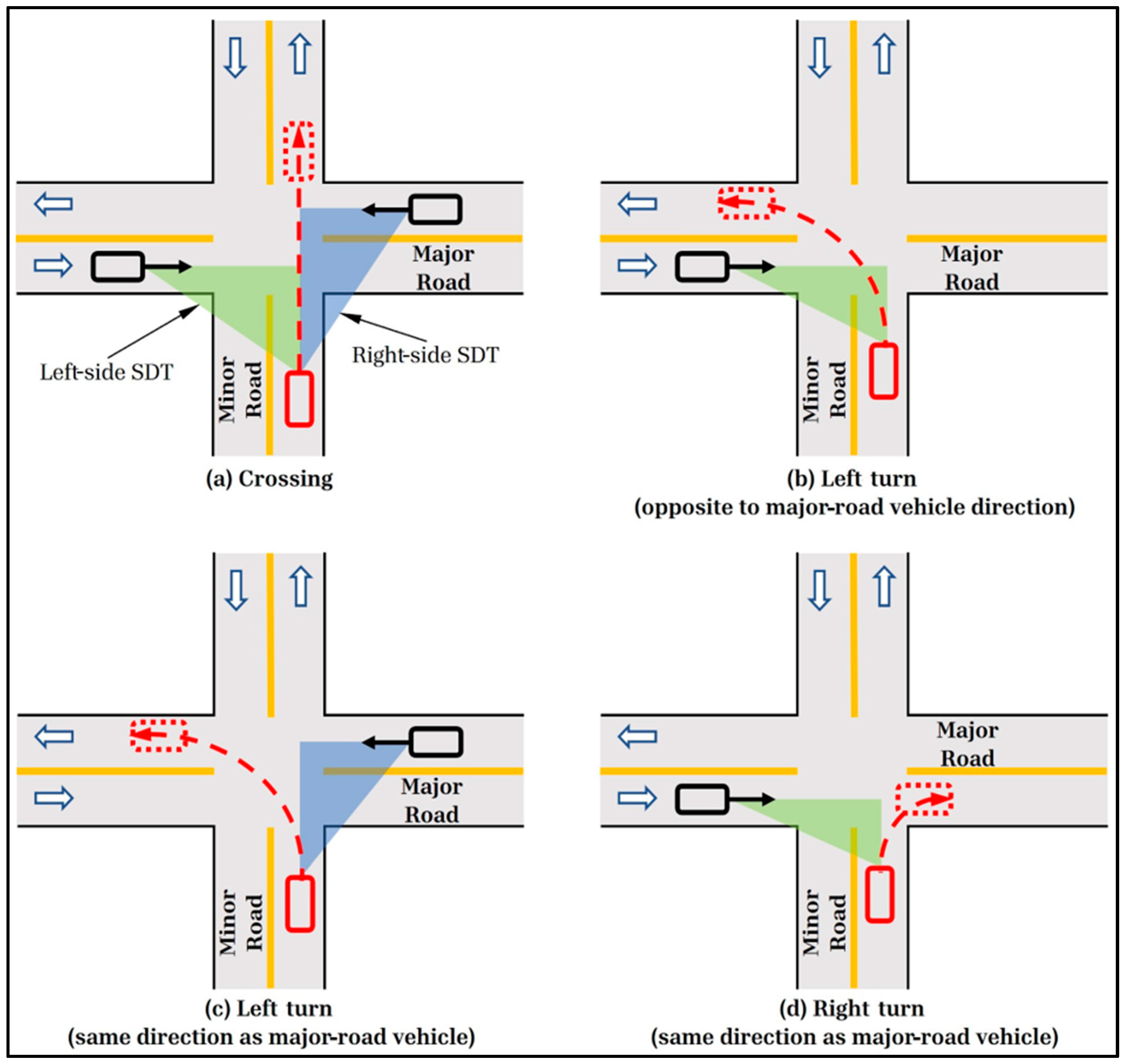
2.2. Conflict Analysis

Different conflicts can develop between the minor- and major-road vehicles on a general four-leg intersection. Focusing on the minor-road vehicle maneuver, Figure 2 shows the possible conflict types between minor- and major-road vehicles. First, Figure 2a illustrates that a minor-road vehicle traveling through the intersection and crossing the major road can conflict with vehicles on both major-road approaches. In this case, the minor-road vehicle needs to clear the paths of the conflicting major-road vehicles approaching from both sides, and analysis would require right- and left-side SDTs. Second, a minor road turning left may conflict with a major-road vehicle traveling in a direction opposite to the direction of the minor-road vehicle after the turning. As shown in Figure 2b, this conflict involves a major-road vehicle approaching from the left side. Similarly to the crossing conflicts, the minor-road vehicles need only to clear the path of the conflicting major-road vehicle, and analysis would require only a left-side SDT. Finally, a minor road turning left or right may conflict with a major-road vehicle traveling in the same direction as the minor-road vehicle after the turning. Figure 2c,d show that this conflict can develop between a left-turning minor-road vehicle and a major-road vehicle approaching from the right side or a right-turning minor-road vehicle and a major-road vehicle approaching from the left side. In this case, a safe maneuver requires the minor-road vehicle to complete the turning maneuver, accelerate to a reasonable speed, and keep an appropriate time gap ahead of the conflicting major-road vehicle. The analysis would require right- and left-side SDTs. Thus, at a typical four-leg intersection with all movements allowed, five different conflict types can develop between minor-road and major-road vehicles:

• The crossing-right side (CRS) involves a-minor-road vehicle and a major-road vehicle approaching from the right side.
• The crossing-left side (CLS) involves a minor-road vehicle and a major-road vehicle approaching from the left side.
• The left turn-left side (LTLS) involves a left-turning minor-road vehicle and a major-road vehicle approaching from the left side.
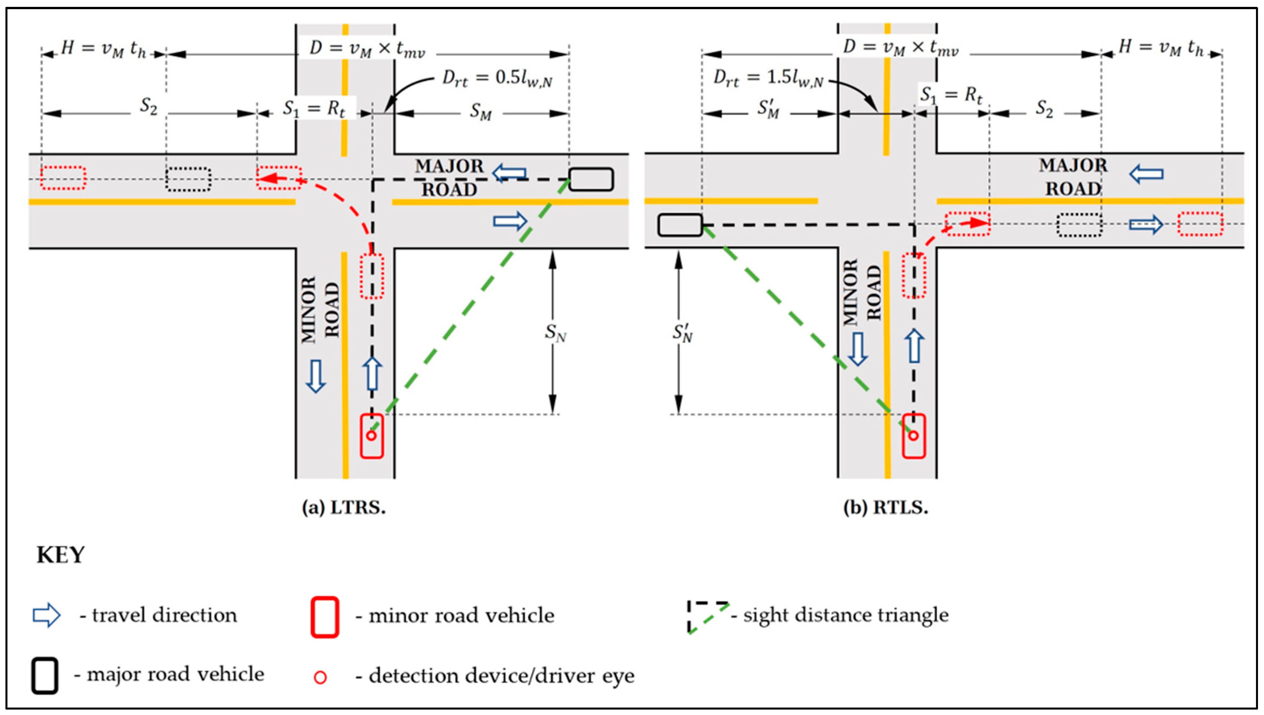
• The left turn-right side (LTRS) involves a left-turning minor-road vehicle and a major-road vehicle approaching from the right side.
• The right turn-left side (RTLS) involves a right-turning minor-road vehicle and a major-road vehicle approaching from the left side.

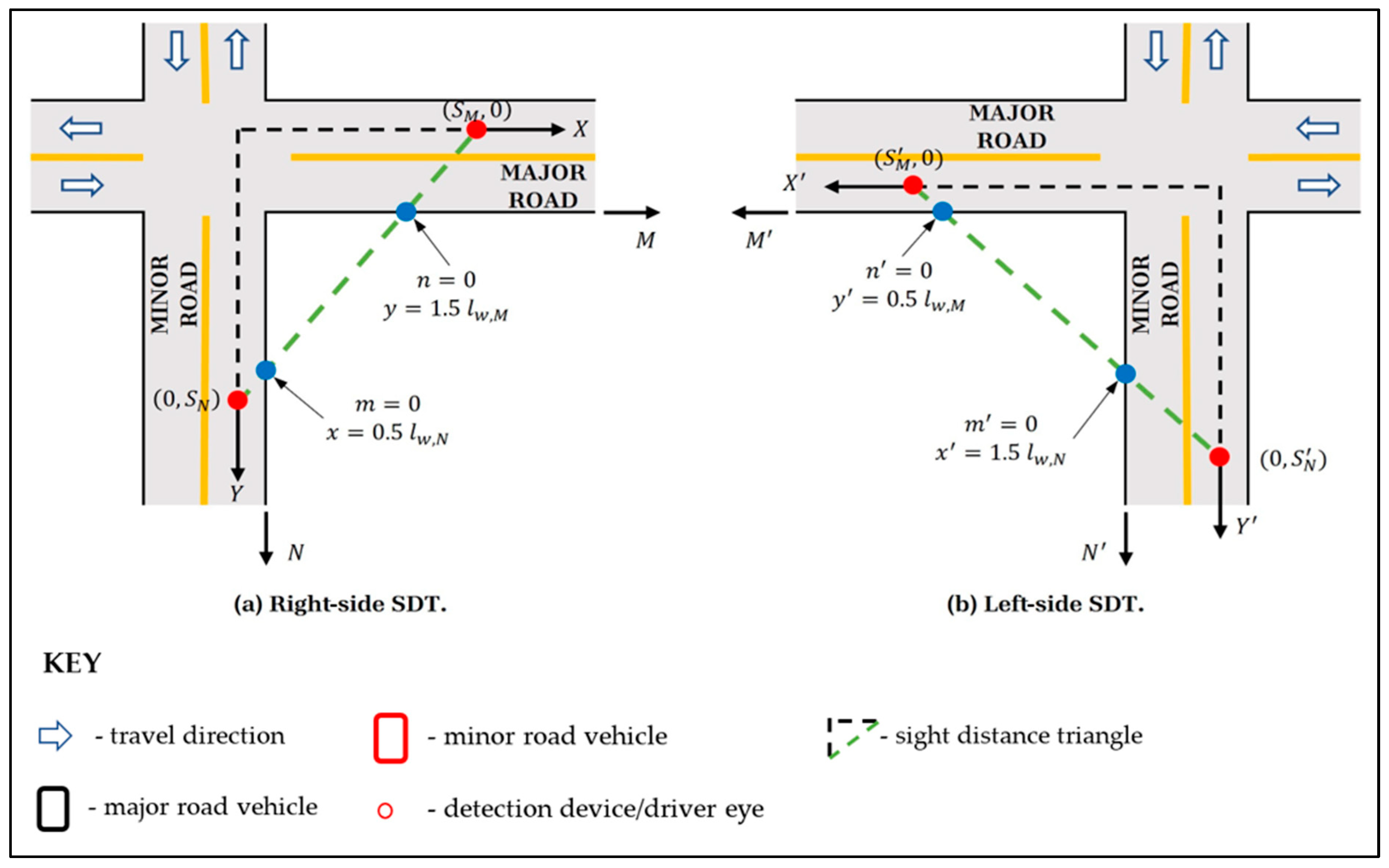
The abbreviations used to denote these conflict types identify the minor-road vehicle’s maneuver (C = crossing, RT = right turn, or LT = left turn) and the direction of the major-road approach which is the same as the SDT direction (RS = right side or LS = left side).

A Poisson-based model has been used in the literature to estimate the number of conflicts at a yield-controlled intersection due to its applicability to such low-volume intersections [3,10,11]. According to this model, the number of conflicts at yield-controlled intersections is a function of the average daily traffic (ADT) volumes on the intersecting roads, and a conflict would exist if two vehicles arrive within a specific time (t) of each other [3]. The shares of each vehicle type and turning or crossing percentages are factored into the model since the ISD analysis for these intersection types considers the various vehicle maneuvers from the minor roadway. Equation (1) models the number of daily vehicle conflicts for any maneuver on the minor road depending on the conflicting volume on the major road and assuming that all the daily traffic volume practically arrives in an 18 h (64,800 s) period and the interarrival time threshold for a conflict, $t$ = 2 s.

$${N_c}_i={P_{M}V}_M\left({\displaystyle \frac{{{P_{m}P}_{N}V}_{N}t}{T}}\right)e^{-\left({\displaystyle \frac{{{P_{m}P}_{N}V}_{N}t}{T}}\right)}$$

(1)

where ${N_c}_i$ = the number of daily conflicts for a specific interaction and conflict type, $P_M$ = the share of vehicle types under consideration on a major road, $P_N$ = the share of vehicle types under consideration on the minor road, $P_m$ = the percentage of maneuver types, $V_M$ and $V_N$ = the one directional ADT on the analysis approach of the major and minor roads (veh/d), $t$ = the interarrival time of the vehicles on the intersecting approaches (s), and $T$ = the total time during an 18-hour period in seconds.

2.3. SDT Properties

If all movements are allowed on the minor road (crossing, right turn, and left turn), different SDTs need to be analyzed for each movement or maneuver as mentioned earlier. Figure 3 shows the typical right- and left-side SDTs that can be used to analyze potential conflicts at a yield-controlled intersection. The lengths A (or A’) and B (or B’) represent the SDT legs on the major and minor roads, respectively, where the accent (’) denotes the left-side SDT parameters. The location of an object representing a potential sight obstruction is denoted by distances m (or m’) and n (or n’) from the near edges of the minor and major roads, respectively. Based on the geometry, the distances a (or a’) and b (or b’) from the sight obstruction to the SDT legs on the minor and major roads, respectively, can be defined for the various vehicle interaction scenarios using the relations in

Table 1. SDT Geometric relationships of SDTs.

Interaction	Right-Side SDT	Left-Side SDT
DVN/DVM	$A=S_M+l_{w,N}-x_N-y$ $B=S_N+z+l_{w,M}+x_M+0.5w$ $a=m+l_{w,N}-x_N-y$ $b=n+l_{w,M}+x_M+0.5w$	$A=S_M^{\prime }+l_{w,N}+x_N+y$ $B=S_N^{\prime }+z+l_{w,M}-x_M-0.5w$ $a=m^{\prime }+l_{w,N}+x_N+y$ $b=n^{\prime }+l_{w,M}-x_M-0.5w$
DVN/AVM	$A=S_M+l_{w,N}-x_N-y$ $B=S_N+z+1.5w$ $a=m+l_{w,N}-x_N-y$ $b=n+1.5l_{w,M}$	$A=S_M^{\prime }+l_{w,N}+x_N+y$ $B=S_N^{\prime }+z+0.5l_{w,M}$ $a=m^{\prime }+l_{w,N}+x_N+y$ $b=n^{\prime }+0.5l_{w,M}$
AVN/DVM	$A=S_M+{0.5l}_{w,N}$ $B=S_N+r+l_{w,M}+x_M+0.5w$ $a=m+{0.5l}_{w,N}$ $b=n+l_{w,M}+x_M+0.5w$	$A=S_M^{\prime }+{1.5l}_{w,N}$ $B=S_N^{\prime }+r+l_{w,M}-x_M-0.5w$ $a=m^{\prime }+{1.5l}_{w,N}$ $b=n^{\prime }+l_{w,M}-x_M-0.5w$
AVN/AVM	$A=S_M+{0.5l}_{w,N}$ $B=S_N+r+{1.5l}_{w,M}$ $a=m+{0.5l}_{w,N}$ $b=n+{1.5l}_{w,M}$	$A=S_M^{\prime }+{1.5l}_{w,N}$ $B=S_N^{\prime }+r+{0.5l}_{w,M}$ $a=m^{\prime }+{1.5l}_{w,N}$ $b=n^{\prime }+{0.5l}_{w,M}$

$A$ and $B$ = the length of the SDT leg along the major and minor roads, $a$ and $b$ = the distance from the object to the SDT leg along the major and minor roads, $S_M$ and $S_N$ = the ISD on the major and minor roads, $m$ and $n$ = the distance from an object to the outer edge of the major and minor roads, $l_{w,M}$ and $l_{w,N}$ = the lane width of the major and minor roads, $x_M$ and $x_N$ = the lateral distance from the left edge of the major- and minor-road lanes to the left side of the traversing vehicle, $z$ = the distance from a DV’s front bumper to the driver’s eye, $r$ = the distance from an AV’s front bumper to an AV’s detection device, $w$ = DV width, and $y$ = the lateral distance from the left side of the vehicle to the driver’s eye.

. It should be noted that the SDT leg along the minor road passes by the vehicle’s detection point, while the SDT leg along the major road coincides with the vehicle’s center. AVs are assumed to be centered in their lanes.

2.4. ISD Models

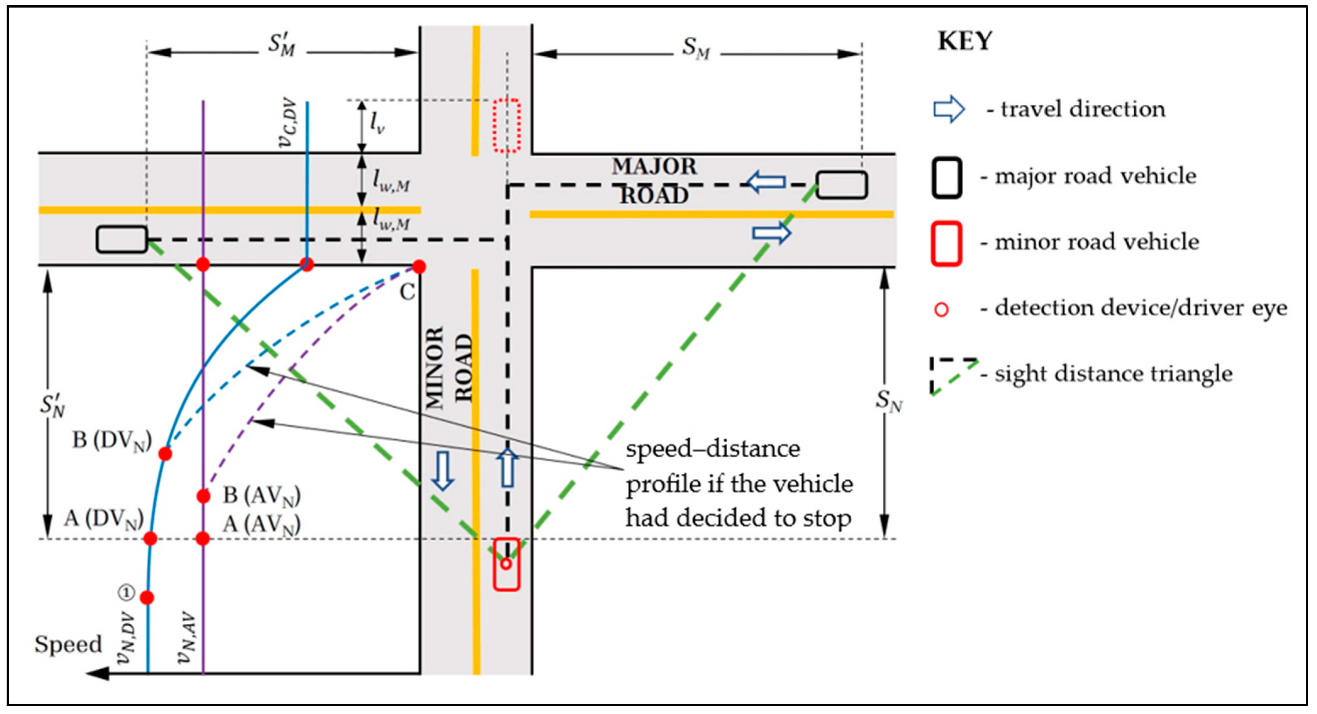
2.4.1. Minor-Road Models

A minor-road vehicle may enter the intersection and execute the required crossing or turning maneuver without stopping if acceptable gaps are detected in the major road. Otherwise, the minor-road vehicle should yield the right of way by slowing down and stopping, and therefore the ISD model is based on providing stopping sight distance (SSD) on the minor road. However, Harwood et al. [3], noted that the field data show that DVs slow down at a relatively low deceleration rate, referred to as the initial deceleration rate ($a_i$), when approaching a yield-controlled intersection regardless of the presence of a conflicting major-road vehicle. If the minor-road DV (DV_N) does not encounter a conflict with major-road vehicles, it proceeds to cross the intersection at a reduced speed of approximately 60% of the midblock speed. This scenario is illustrated in Figure 4a, where the DV_N only slows down to a lower crossing speed ($v_{c,DV}$) in the case of crossing or to a safe turning speed ($v_{t,DV}$) in the case of a left or right turn with deceleration taking place between Points ➀ and ➁. In this paper, $v_{c,DV}$ is not fixed at a specific value or specific ratio but is rather determined by applying a variable reduction factor ($f_r$) to the midblock speed ($v_{N,DV}$). Finally, Harwood et al. [3] noted the minimum, maximum, and mean speed reduction as observed in field studies (0, 100, and 36.5%, respectively) but not the distribution of this speed reduction. It is assumed that $f_r$ follows a triangular distribution, which is defined by three values of the minimum (a = 0), maximum (c = 1), and peak location b and which was calculated as 0.095 using the information of the mean (µ = 0.365), a, and b using the following equation [12]:

$$\mu ={\displaystyle \frac{a+b+c}{3}}$$

(2)

On the other hand, if a conflict is perceived, the DV_N would need to apply the brakes harder to slow down at a braking rate (a_b) and stop before the intersection. Therefore, the ISD for the DV_N is equivalent to the distance traveled during the perception–reaction time (PRT) and braking. In general, there are three possible scenarios for how far back the driver of the DV_N needs to decide to stop and apply the brakes as illustrated in Figure 4b–d. The important points to note in these speed profiles are as follows:

• Point A: the decision point and beginning of the PRT.
• Point B: the end of the PRT and the beginning of the braking distance.
• Point C: the end of the braking distance and the beginning of the intersection. The location of Point C coincides with Point ➁, with both points coinciding with the beginning of the intersection.

In these speed profiles, it is assumed that the DV_N’s original profile does not change during the PRT (from A to B). To model the DV_N’s ISD, and based on the observed pattern of DV speeds at yield-controlled intersections, the speed at Point C if there is no conflict (v_c) can be written as follows:

$$v_c=\left\{\begin{array}{c}{v}_{c,DV}=f_r{v}_{N,DV} if crossing {DV}_N\hfill \\ v_{t,DV} if turning {DV}_N \hfill \end{array}\right.$$

(3)

where $f_r$ = the speed reduction factor, $v_{n,DV}$ = the DV_N’s midblock speed, and $v_{t,DV}$ = the DV_N’s turning speed.

Based on the distance–speed–acceleration relationships, it can be shown that

$$v_b=min\left(\sqrt{v_c^2+a_i{\displaystyle \frac{v_c^2}{a_b-a_i}}},v_{N,DV}\right)$$

(4)

$$v_a=min\left(v_c^2+a_i{t}_{pr},v_{N,DV}\right)$$

(5)

$$v_c=\left\{\begin{array}{c}{\displaystyle \frac{v_c^2}{2(a_b-a_i)}} if Scenario 1 or 2: v_a<v_{N,DV} \hfill \\ {\displaystyle \frac{v_{N,DV}^2}{2a_b}} if Scenario 3: v_b=v_a=v_{N,DV}\hfill \end{array}\right.$$

(6)

$$v_c=\left\{\begin{array}{c}{v}_b{t}_{pr}+{0.5a}_i{t}_{pr}^2 if Scenario 1: v_a<v_{N,DV} \\ v_d{t}_{pr}-{\displaystyle \frac{v_{N,DV}^2-v_b^2}{2a_i}} if Scenario 2: v_b<v_{N,DV},v_a=v_{N,DV} \\ v_d{t}_{pr} if Scenario 3: v_b=v_a=v_{N,DV} \end{array}\right.$$

(7)

$$S_{N,DV}=X_{pr}+X_b$$

(8)

where $S_{N,DV}$ = the DV_N’s ISD, $X_b$ = the braking distance if the DV_N has to stop due to a conflict, $X_{pr}$ = the distance traveled by the DV_N during the PRT, $v_a$ and $v_b$ = the DV_N’s speed at Points A and B, $a_i$ = the DV_N’s initial deceleration rate before braking, $a_b$ = the DV_N’s deceleration rate when braking, and $t_{pr}$ = the driver’s PRT.

If the minor-road vehicle is an AV (AV_N), Sarran and Hassan [9] contended that it will be less efficient for the AV_N to slow down without the presence of a conflicting vehicle. Therefore, the AV_N’s ISD in this paper is based on the SSD from the midblock speed as shown in Equation (9). For turning maneuvers, the AV_N needs to slow down to a safe turning speed. However, the AVs are assumed to have the same deceleration rate for slowing down or stopping, and therefore an AV_N’s decision to stop must be made at a distant equivalent to the SSD from the midblock speed before the intersection. Subsequently, the same equation is applicable to both the crossing and turning maneuvers.

$$S_{N,AV}=v_{N,AV}{t}_{dr}+{\displaystyle \frac{v_{N,AV}^2}{2a_a}}$$

(9)

where $S_{N,AV}$ = the AV_N’s ISD, $v_{N,AV}$ = the AV_N’s midblock speed, $a_a$ = the AV_N’s braking rate, and $t_{dr}$ = the AV detection and reaction time (DRT).

2.4.2. Major-Road Models

At yield-controlled intersections, the ISD along the major roadway depends on the behavior of both the major- and minor-road vehicles. For the current DV model, the ISD on the major road is computed using the speed of the vehicle on the major-road approach and a time gap ($t_g$) that would be accepted by the minor-road vehicle to complete the maneuver [3] as follows:

$$S_M=\left\{\begin{array}{c}{v}_{M,DV}{t}_g if {DV}_M \\ v_{M,AV}{t}_g if {AV}_M \end{array}\right.$$

(10)

where $S_M$ = the ISD along the major roadway and $v_{M,DV}$ and $v_{M,AV}$ = the major road’s DV and AV speeds.

The same approach is used in this paper, but the process to estimate $t_g$ depends on whether the minor-road vehicle is a DV or an AV (i.e., whether the case is a DV_N or an AV_N). The requirements for the major-road $t_g$ and ISD also vary by the maneuver type and potential conflict. Consequently, different models were developed for the different vehicle interaction and conflict types.

Crossing Maneuver (CRS and CLS)

Harwood et al. [3] modeled $t_g$ for a minor-road vehicle crossing the intersection as the total time required for the vehicle to travel from the decision point (denoted as Point A in Figure 4) to the point where it completely crosses the major road. In a mixed vehicle fleet, this time depends on the type of minor-road vehicle that performs the crossing maneuver. Figure 5 illustrates the SDTs for the right- and left-side-crossing conflicts (CRS and CLS) and the speed profile for the DV_N and AV_N. Only Scenario 1 of the DV_N speed profile is shown to reduce the figure complexity. As shown in the figure, $t_g$ can be broken down into four components as follows:

• The travel time between Points A and B ($t_{A-B}$) is equal to the PRT or DRT ($t_{pr}$ or $t_{dr}$) for the DV_N or AV_N, respectively.
• The travel time between Point B and the beginning of the intersection (Point ➁ or C) follows the original speed profile with no stopping ($t_{B-C}$).
• The travel time to cross the major road: for the CLS and two-lane major roads, the minor-road vehicle needs to clear only one major-road lane, while it has to clear both lanes for the CRS.
• The travel time is shown for a distance equivalent to the vehicle length ($l_v$).

As mentioned earlier, an AV_N that does not encounter a conflict is assumed to travel at a constant speed $S_{N,AV}$ without slowing down. Therefore, the four time components can be combined, and $t_g$ can be directly calculated using the distance from the decision point to the beginning of the intersection ($S_{N,AV}$), the intersection width to be cleared, and the vehicle length as formulated later in Equation (13). On the other hand, for the DV_N, $t_{B-C}$ can be formulated based on the speed profile scenario as follows:

$$S_M=\left\{\begin{array}{c}{\displaystyle \frac{v_b-v_c}{a_i}} if Scenario 1 or 2: v_b<v_{N,DV} \\ {\displaystyle \frac{v_{N,DV}}{2a_b}}-{\displaystyle \frac{v_{N,DV}^2-v_c^2}{2{v_{N,DV}a}_i}}+{\displaystyle \frac{v_{N,DV}-v_c}{a_i}} if Scenario 3: v_b=v_a=v_{N,DV} \end{array}\right.$$

(11)

where $v_b$ = the DV_N at Points B (Equation (4)), and $v_c$ = the DV_N at Points C (Equation (3)).

For the travel time to cross the intersection and travel an additional distance of l_v, Harwood et al. [3] assumed that the vehicle would travel at a constant speed. This assumption was also adopted in this paper for the cases of an AV_N (traveling at $v_{N,AV}$) and DV_N if the speed reduction was not very high. However, a DV_N would be expected to accelerate while crossing the intersection if it had slowed down to a very slow speed or stopped before the intersection (refer to $f_r$ distribution in Equation (2)). In this paper, a DV_N was assumed to maintain a constant crossing speed $v_{c,DV}$ if $f_r$ was in the lower 85th percentile of the cumulative frequency distribution. Otherwise, a DV_N with a high $f_r$, with the threshold assumed as the top 15th percentile, was assumed to accelerate during crossing using the same acceleration rate $a_d$. The value of $f_r$ corresponding to this threshold was termed a critical speed reduction factor $f_{cr}$ and was calculated as 0.6316 using Matlab’s built-in function “cdf” or the following equation for the cumulative frequency distribution of a triangular distribution for a value in the range [b, c] [12]:

$$0.85=1-{\displaystyle \frac{{\left(c-f_{cr}\right)}^2}{\left(c-a\right)\left(c-b\right)}}$$

(12)

Thus, $t_g$ for the crossing maneuver can be formulated as shown in Equation (13). Assuming that the major-road vehicle travels at a constant speed, the major-road ISD can be calculated using Equation (10).

$$t_g=\left\{\begin{array}{c}{t}_{pr}+t_{B-C}+{\displaystyle \frac{\sqrt{{v_{c,DV}^2+2a}_i{D}_c}-v_{c,DV}}{a_d}} if {DV}_N and v_{c,DV}<{f_{cr}v}_{N,DV} \hfill \\ t_{pr}+t_{B-C}+{\displaystyle \frac{D_c}{v_{c,DV}}} if {DV}_N and v_{c,DV} \ge {f_{cr}v}_{N,DV} \hfill \\ {\displaystyle \frac{S_{N,AV}+D_c}{v_{N,AV}}} if {AV}_N \hfill \end{array}\right.$$

(13)

$$D_c=\left\{\begin{array}{c}{2l}_{w,M}+l_v if CRS \\ l_{w,M}+l_v ifCLS \end{array}\right.$$

(14)

where $D_c$ = the total crossing distance; $l_{w,M}$ = the major-road lane width; and $l_v$ = the length of the minor-road vehicle, which is equal to $l_{v,DV}$ or $l_{v,AV}$ for a DV_N or an AV_N.

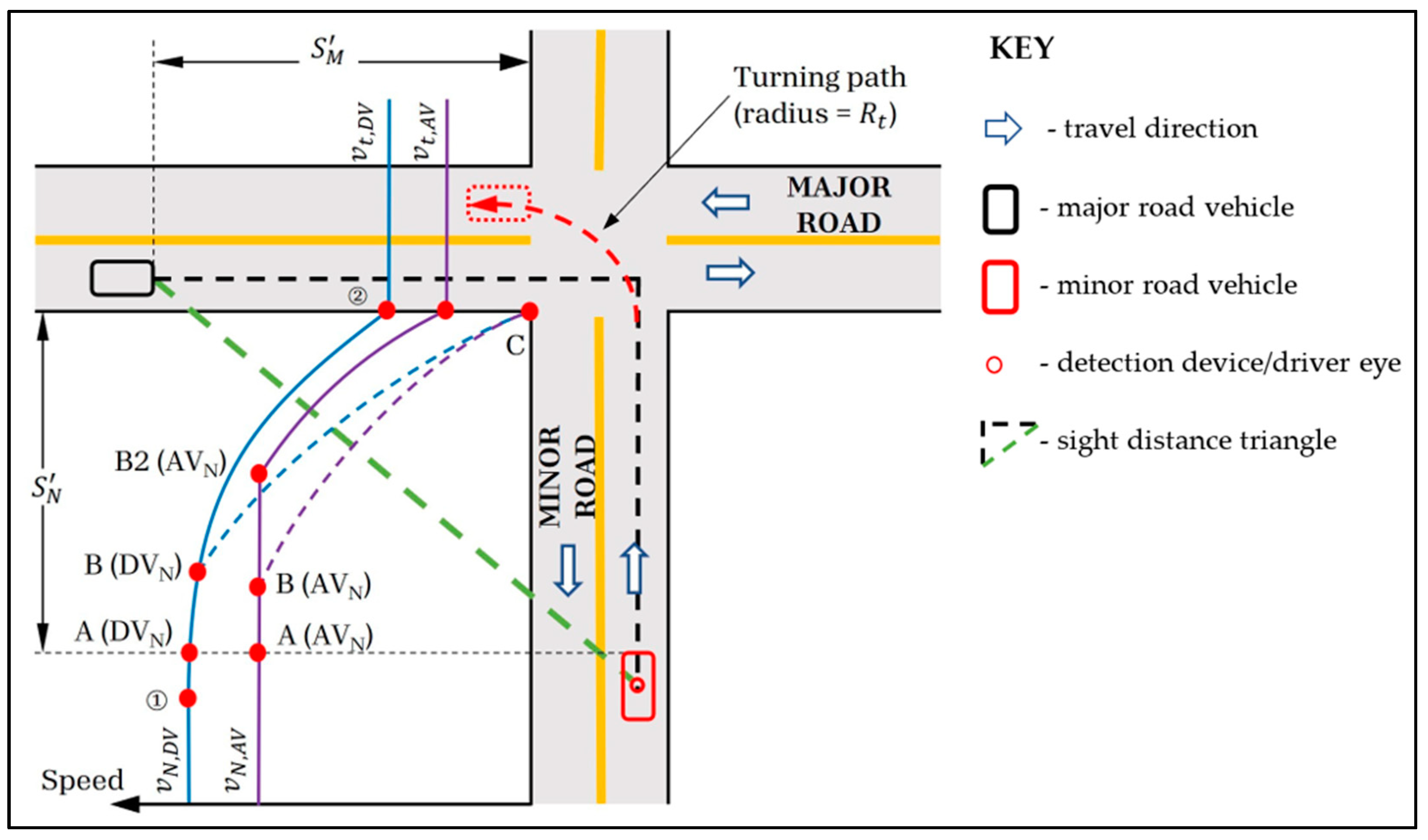
Turning Opposite to Major-Road Traffic (LTLS)

When a minor-road vehicle turns left, it needs also to clear the major-road vehicles approaching from the left side, which is opposite to the turning road’s final travel direction. This conflict was denoted earlier as the LTLS. Similarly to the crossing maneuver, the associated time with this left-turn maneuver starts from the decision point until the minor-road vehicle completes the turning onto the major road. As shown in Figure 6, $t_g$ for a turning DV_N can be derived following the same logic in the CLS and CRS, while using the turning speed ($v_{t,DV}$) in place of the crossing speed ($v_{c,DV}$). However, when the DV_N reaches the beginning of the intersection, the additional distance to clear the intersection is approximately a circular arc equivalent to a quarter of a circle with radius R_t as shown in Figure 6. In addition, $v_{t,DV}$ was assumed to follow a narrower distribution than $v_{c,DV}$, and therefore the assumption of constant speed is reasonable. A turning AV_N is also needed to slow down to a safe turning speed ($v_{t,AV}$) using the same deceleration rate ($a_a$) starting from a new point in the speed profile shown in Figure 6 as B2. Subsequently, $t_g$ for the AV_N can be formulated as the sum of travel times from the decision point (Point A) to Point B2 at a constant speed $v_{N,AV}$, during deceleration between Points B2 and C, and during turning at a constant speed $v_{t,AV}$. Following the distance–speed–acceleration relationships, the models for the major-road $t_g$ and LTLS conflict are shown in Equation (15), and the major-road ISD can then be calculated using Equation (10).

$$t_g=\left\{\begin{array}{c}{t}_{pr}+t_{B-C,t}+{\displaystyle \frac{0.5\pi R_t}{v_{t,DV}}} if {DV}_N and LTLS \\ t_{dr}+{\displaystyle \frac{v_{t,AV}^2}{2{v_{N,AV}a}_a}}+{\displaystyle \frac{v_{N,AV}-v_{t,AV}}{a_a}}+{\displaystyle \frac{0.5\pi R_t}{v_{t,AV}}} if {AV}_N and LTLS \\ \end{array}\right.$$

(15)

where $v_{t,DV}$ and $v_{t,AV}$ = the major road’s DV and AV turning speeds, $t_{B-C,t}$ = the DV_N’s travel time between Points B and C to be estimated using Equations (4) and (11) and setting $v_c$ = $v_{t,DV}$ as per Equation (3), and $R_t$ = the effective turning radius of the minor-road vehicle.

Turning in the Same Direction as Major-Road Traffic (LTRS and RTLS)

The required ISD along the major road when the minor-road vehicle turns right or left in the direction of the major-road traffic (denoted as LTRS and RTLS conflicts) can also be modeled based on the required $t_g$ on the major road. For a DV_N, Harwood et al. [3] based their approach on the required $t_g$ at yield-control intersections on the accepted $t_{g,s}$ by drivers turning at stop-controlled intersections as measured in the field. The measured $t_{g,s}$ is then modified to account for the travel time along the minor road and the time lost for accelerating from rest to turning speed. A constant $t_g$ value of 8.0 s based on this logic has been adopted in the Green Book [1]. The same logic was attempted in this paper to develop a general model for the $t_g$ turning DV_N. However, many combinations of the vehicle speed, acceleration, and deceleration parameters were found to produce unreasonable, and even negative, $t_g$ values. Therefore, the approach by Dabbour [13] and Dabbour and Easa [14] was adopted to estimate the time required for a turning vehicle to turn and accelerate while maintaining a safe distance from the following vehicle.

As shown in Figure 7, the turning vehicle first travels from the decision point to the intersection and then turns at a constant speed, and the time taken is similar to that estimated for the LTLS. The turning vehicle then travels along the major road for a distance $S_2$ while accelerating to a final speed depending on the major-road speed limit. Thus, the total maneuver time can be formulated as follows:

$$t_{mv}=\left\{\begin{array}{c}{t}_{pr}+t_{B-C,t}+{\displaystyle \frac{0.5\pi R_t}{v_{t,DV}}}+{\displaystyle \frac{v_{M,DV,t}-v_{t,AV}}{a_d}} if {DV}_N \\ t_{dr}+{\displaystyle \frac{v_{t,AV}^2}{2{v_{N,AV}a}_a}}+{\displaystyle \frac{v_{N,AV}-v_{t,AV}}{a_a}}+{\displaystyle \frac{0.5\pi R_t}{v_{t,AV}}}+{\displaystyle \frac{v_{M,AV,t}-v_{t,AV}}{a_c}} if {AV}_N \\ \end{array}\right.$$

(16)

where $t_{mv}$ = the total maneuver time when turning in the same direction of a major-road vehicle, $v_{M,DV,t}$ and $v_{M,AV,t}$ = the final speed of a DV_N and an AV_N after turning and accelerating on the major road, and $a_d$ and $a_c$ = the acceleration rate of a DV_N and an AV_N after turning.

As the turning vehicle completes the maneuver, the major-road vehicle will have traveled a distance D to a final position that is a distance H behind the turning minor-road vehicle to allow for a minimum headway between the two vehicles. Thus, $t_g$ is estimated as $t_{mv}$ minus the travel time of the major-road vehicle after the near edge of the minor road. Following the speed–distance–acceleration relationships and geometric relationships in Figure 7, the models for $t_g$ for the LTRS and RTLS are formulated as shown in Equation (17), and the major-road ISD can be calculated using Equation (10).

$$t_g=\left\{\begin{array}{c}{t}_{mv}+t_{h,DV}-{\displaystyle \frac{R_t+D_{rt}}{v_{M,DV}}}-{\displaystyle \frac{v_{M,DV,t}^2-v_{t,DV}^2}{2{v_{M,DV}a}_c}} if {DV}_N and {DV}_M \hfill \\ t_{mv}+t_{h,AV}-{\displaystyle \frac{R_t+D_{rt}}{v_{M,AV}}}-{\displaystyle \frac{v_{M,DV,t}^2-v_{t,DV}^2}{2{v_{M,AV}a}_c}} if {DV}_N-{AV}_M \\ t_{mv}+t_{h,DV}-{\displaystyle \frac{R_t+D_{rt}}{v_{M,DV}}}-{\displaystyle \frac{v_{M,AV,t}^2-v_{t,AV}^2}{2{v_{M,DV}a}_c}} if {AV}_N-{DV}_M \\ t_{mv}+t_{h,AV}-{\displaystyle \frac{R_t+D_{rt}}{v_{M,AV}}}-{\displaystyle \frac{v_{M,AV,t}^2-v_{t,AV}^2}{2{v_{M,AV}a}_c}} if {AV}_N-{AV}_M \end{array}\right.$$

(17)

$$D_c=\left\{\begin{array}{c}{0.5l}_{w,N} if LTRS \\ 1.5l_{w,M} ifRTLS \end{array}\right.$$

(18)

where $D_{rt}$ the distance from the major road edge to the SDT leg on the minor road, and $t_{h,DV}$ and $t_{h,DV}$ = the time headway between the turning AV_N and the following DV_M or AV_M.

2.5. System Models

Easa [4] proposed combining the relevant parameters into one variable to evaluate the ISD supply and demand in relation to object distances relative to minor and major roads. This variable, known as the corner distance, is the distance from an object location to the point at which the minor and major SDT legs intersect and is shown as $D_s$, $D_d$, ${D_s}^{\prime }$, and ${D_d}^{\prime }$ in Figure 3. Easa [4] formulated $D_s$ and $D_d$ for the right-side SDTs in terms of the other geometric parameters as follows:

$$D_s=\sqrt{a^2+b^2}$$

(19)

$$D_d={\displaystyle \frac{A\times B}{A\sin \left({\tan }^{-1}\frac{b}{a}\right)+B\cos \left({\tan }^{-1}\frac{b}{a}\right)}}$$

(20)

where $D_s$ and $D_d$ = supply and demand corner distances, $A$ and $B$ = the length of the SDT leg along major and minor roads, and $a$ and $b$ = the distance from the object to the SDT leg along major and minor roads.

For the left-side corner distances, the distances $a$, $b$, $A$, and $B$ should be replaced by $a^{\prime }$, $b^{\prime }$, $A^{\prime }$, and $B^{\prime }$, respectively. Using the supply and demand corner distances, the system’s performance function Z can be written as follows:

$$Z=D_s-D_d$$

(21)

2.6. Probabilistic Assessment

The probability of non-compliance (PNC) has been used as a measure of the system demand exceeding the system supply in many transportation engineering applications [15]. The developed ISD models can be combined with the system’s performance function to compute the PNC at a yield-controlled intersection for a specific object location, vehicle interaction type, and conflict type. Among the methods available to compute the PNC, Monte Carlo Simulation (MCS) is a repeated random sampling reliability approach that can be applied with accuracy in many cases requiring probabilistic analysis [16]. Therefore, it has been widely adopted for reliability analysis [17] and was selected as the PNC evaluation method in this study.

According to Singh et al. [18], MCS’s accuracy hinges on the number of simulations performed. At a minimum, the number of simulation runs should be 5000. Previous MCS-based highway design studies used a number of simulations that is as high as 100,000 [17,19] and 150,000 [15]. Using such high values of simulation runs leads to an acceptable, low-MCS standard error of the estimates or PNC coefficient of the variation values [15,17]. Using these values as a benchmark, the number of runs selected for this study was 200,000, a value in line with another study [9]. Having defined the distributions of the different models’ parameters, each simulation run computed the difference between $D_s$ and $D_d$ for the randomly selected parameter values. Non-compliance or failure in the simulation was defined as a negative value of the performance function ($Z$), and the PNC for a specific vehicle interaction could then be calculated as follows:

$${PNC}_i={\displaystyle \frac{F_i}{N}}$$

(22)

where ${PNC}_i$ = the PNC for a specific combination $i$ of vehicle interaction and maneuver types, $F_i$ = the number of failures for interaction $i$, $N$ = the number of simulation runs.

It should be noted that the PNC reflects the probability of failed conflicts. However, some minor-road vehicles may be conflict-free, and therefore ISD failure would not occur regardless of the actual supply and demand ISD. This is particularly true for intersections with low-traffic volumes such as yield-controlled intersections. Thus, Sarran and Hassan [9] proposed a better measure of failure as the number of unresolved conflicts (PUC), which refers to those conflicts that need evasive action by at least one vehicle beyond the identified driving behavior values to prevent a collision. Therefore, the PNC is combined in this study with the results of a conflict assessment (Section 2.2) to form the measure PUC to reflect the probability of failure or unresolved conflict relative to the traffic volume. The total number of unresolved conflicts can be found by summing the number of conflicts of all the interactions that experience a demand ISD greater than the supply or a negative performance function $Z$. The PUC is then calculated as the ratio of the total number of unresolved conflicts to the daily volume on the minor road as shown in Equation (23). It should be noted that any conflict involves a pair of vehicles on minor and major roads. Therefore, the ratio in Equation (23) is based on the lower volume on the minor road. It should also be noted that when a volume is involved in multiple conflicts (for example through the volume that is involved in the CRS and CLS), this volume is included only once in the denominator of Equation (23).

$$PUC={\displaystyle \frac{{\sum }_i{PNC}_i\times {N_c}_i}{{\sum }_i{V}_i}}$$

(23)

where $PUC$ = the probability of an unresolved conflict, ${PNC}_i$ = the PNC for a specific combination $i$ of vehicle interaction and maneuver types, ${N_c}_i$ = the number of daily conflicts for a combination $i$, $V_i$ = the minor-road vehicle volume involved in combination $i$ (veh/d).

2.7. Target PUC

Ideally, ISD adequacy should be assessed based on the expected safety performance, in terms of collision frequency, associated with the intersection’s ISD supply. Such an objective safety performance assessment can be achieved by relating the PUC to the collision frequency for a dataset of yield-controlled intersections. However, the typically low volumes, and in turn low collision frequencies, on yield-controlled intersections might make such a relationship difficult to develop. Alternatively, Sarran and Hassan [9] proposed assessing ISD adequacy using a target PUC, which was defined as the maximum PUC that can be experienced in a DV-only environment when the ISD is compliant with the Green Book guidelines [1]. The premise of this target PUC is to provide a similar expected safety level in a mixed AV-DV environment to that currently expected in a DV-only environment. Thus, the target PUC value for a specific intersection is determined as the maximum PUC for all the object locations along the sight line or the hypotenuse of the SDT. This sight line is referred to in this paper as the AASHTO sight line.

The process followed in this study to establish the AASHTO sight line and find the target PUC on a specific intersection is similar to the process developed by Sarran and Hassan [9] for uncontrolled intersections but adopted to account for the different maneuvers at yield-controlled intersections. First,

Table 2. ISD guidelines for crossing maneuvers at yield-controlled intersection [1].

Design Speed (km/h)	${\mathit{S}}_{\mathit{N}}$(m)	${\mathit{t}}_{\mathit{g}}$(s)
20	20	7.1
30	30	6.5
40	40	6.5
50	55	6.5
60	65	6.5
70	80	6.5
80	100	6.5
90	115	6.8
100	135	7.1
110	155	7.4
120	180	7.7
130	205	8.0

$S_N$ = ISD along the minor road. $t_g$ = time gap along the major road.

summarizes the Green Book’s ISD requirements for the crossing maneuver (Tables 9–12 of the AASHTO Green Book [1]). For left- or right-turning maneuvers, and due to the slowing down by turning vehicles, the Green Book recommends a constant ISD on the minor road ($S_N$) of 25 m and constant $t_g$ for a major-road ISD equal to 8.0 s for passenger cars. In all cases, the ISD on the major road is calculated similarly to Equation (10). Possible object locations can be established using the relationship between $m$ and $n$ and between $m^{\prime }$ and $n^{\prime }$ for the right- and left-side SDT, respectively. Using the $X-Y$ (or $X^{\prime }-Y^{\prime }$) coordinate system along the centerlines of the major- and minor-road lanes as shown in Figure 8, the equation of the AASHTO sight line can be established using the coordinates of the two SDT vertices as follows:

$$\begin{gathered} y=S_N-{\displaystyle \frac{S_N}{S_M}}x \\ \acute{y}=S_N-{\displaystyle \frac{S_N}{S_M}}\acute{x} \end{gathered}$$

(24)

where $S_N$ = the ISD along the minor road for the right- or left-side SDT and $S_M$ = the ISD along the major road for the right- or left-side SDT.

$$\begin{gathered} m=x-0.5l_{w,N} ; n=y-1.5l_{w,M} \mathrm{R}\mathrm{i}\mathrm{g}\mathrm{h}\mathrm{t} \mathrm{s}\mathrm{i}\mathrm{d}\mathrm{e} \mathrm{S}\mathrm{D}\mathrm{T} \\ \acute{m}=\acute{x}-1.5l_{w,N} ; \acute{n}=\acute{y}-1.5l_{w,M} \mathrm{R}\mathrm{i}\mathrm{g}\mathrm{h}\mathrm{t} \mathrm{s}\mathrm{i}\mathrm{d}\mathrm{e} \mathrm{S}\mathrm{D}\mathrm{T} \end{gathered}$$

(25)

Equations (24) and (25) can be combined to establish the relationship for object locations along the AASHTO sight line as follows:

$$\begin{gathered} n=S_N-{\displaystyle \frac{S_N}{S_M}}\left(m+0.5l_{w,N}\right)-1.5l_{w,M} \mathrm{R}\mathrm{i}\mathrm{g}\mathrm{h}\mathrm{t} \mathrm{s}\mathrm{i}\mathrm{d}\mathrm{e} \mathrm{S}\mathrm{D}\mathrm{T} \\ \acute{n}=S_N-{\displaystyle \frac{S_N}{S_M}}\left(\acute{m}+1.5l_{w,N}\right)-0.5l_{w,M} \mathrm{L}\mathrm{e}\mathrm{f}\mathrm{t} \mathrm{s}\mathrm{i}\mathrm{d}\mathrm{e} \mathrm{S}\mathrm{D}\mathrm{T} \end{gathered}$$

(26)

Subsequently, object locations are set based on the distance $m$ or $\acute{m}$ ranging from a minimum of 1.0 m and at a 1.0 m interval to a maximum value corresponding to a minimum value of n or n’ just above zero as shown in Figure 8. Finally, the process is performed for both the crossing and turning maneuvers on both the right and left sides. The higher $n$ or$\acute{n}$ value based on crossing and turning for the same value of m or m’ is used to set a possible object location based on the Green Book criteria. Subsequently, the AASHTO sight line as defined in this paper may be a broken line if the controlling maneuver shifts, for example, from crossing to turning.

Finally, in estimating the target PUC, it is noted that the object locations on the right and left sides are not related. Therefore, the maximum overall PUC for the intersection is found by combining the maximum PUC values for both the right- and left-side conflicts. That is, Equation (23) is applied separately to the right-side conflicts (CRS and LTRS) and to the left-side conflicts (CLS, LTLS, and RTLS) at each object location. The maximum values of each of these two combinations are then combined for the maximum intersection PUC value, which is used as the target PUC.

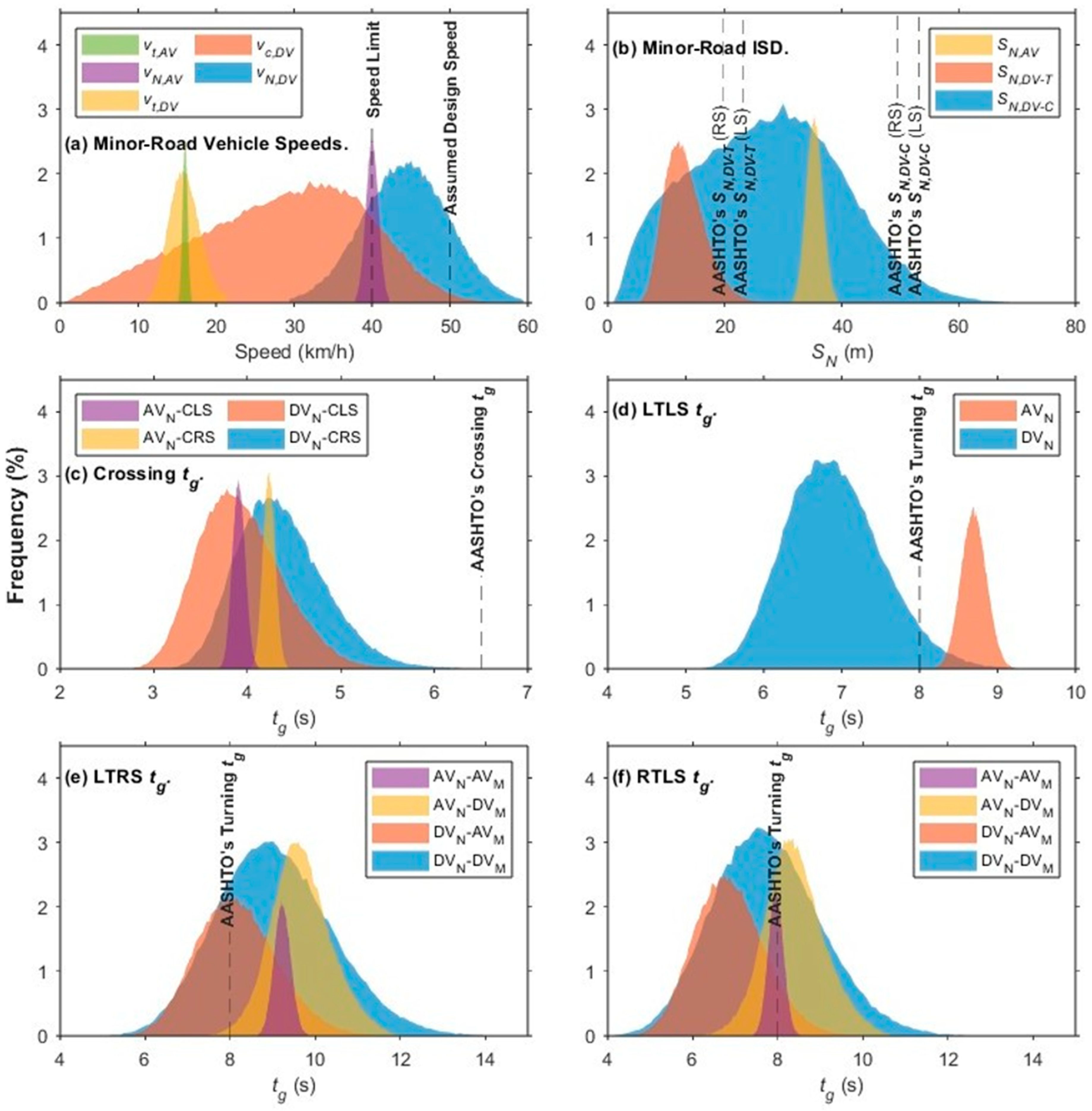
3. Statistical Distributions of Model Parameters

3.1. Driver and Vehicle Parameters

The distributions of the developed model parameters, defined using the mean, standard deviation, shape and scale parameters, minimum and maximum values, peak values, correlation coefficients, and statistical distributions, were obtained directly from the existing literature or through analysis of the collected data. The speed data collected for the DVs showed the mean, mode, and median values having approximately the same value. Such a situation is indicative that the data are normally distributed [9]. For the data collected for the time headway, vehicle length, and vehicle width, the R software 4.2.2 via the “fitdistr” package was used to determine the distributions and associated parameters of the data-based variables. The data for each variable were fitted to various distribution types, which included the lognormal, gamma, exponential, logistic, uniform, Weibull, and t-Location scale. The distributions were assigned based on a Goodness of Fit Test for several distribution types. In this test, the distribution type with the lowest values for Akaike’s Information Criterion (AIC) [20] and the Bayesian Information Criterion (BIC) [21] indicate the best fit [22]. Hence, the distribution with the smallest AIC and BIC values was assigned to an evaluated parameter.

The literature sometimes only provided values associated with specific percentiles and distributions. For the normally distributed cases, the standard deviation and mean values of the associated variables were calculated using the following relationships.

$$\sigma ={\displaystyle \frac{x.CoV}{1+CoV}}$$

(27)

$$\mu =x-z_p.\sigma$$

(28)

where $\mu$ = the mean of the random variable, $x$ = the value of the random variable associated with a certain percentile, $z_p$ = the standardized score, $CoV$ = the coefficient of variation in the random variable, and $\sigma$ = the standard deviation of the random variable.

All the values of the AV parameters were sourced from the existing literature. However, there was a lack of distribution information for these values. It was assumed that the distribution of the AV parameters would follow a normal distribution with the means equal to the sourced values. The variation around the mean was assumed to be small owing to the vehicles’ computerized operations [23], and therefore a small value of 2% was assumed for the coefficient of variation ($CoV$) [9]. The statistical properties of all the relevant DV and AV parameters are summarized in

Table 3. DV parameters.

Design Parameter	Distribution	Statistical Parameters	Source
$v_{N,DV}$, $v_{M,DV}$: speed at 40 km/h posted speed limit	Normal	$\mu$ = 44.20 km/h $\sigma$ = 5.58 km/h	Data
$v_{N,DV}$, $v_{M,DV}$: speed at 50 km/h posted speed limit	Normal	$\mu$ = 53.90 km/h $\sigma$ = 5.85 km/h	Data
$v_{N,DV}$, $v_{M,DV}$: speed at 60 km/h posted speed limit	Normal	$\mu$ = 62.74 km/h $\sigma$ = 7.26 km/h	Data
$v_{t,DV}$: intersection turning speed	Normal *	$\mu$ = 16.00 km/h $\sigma$ = 2.02 km/h **	[3]
$f_r$ speed reduction factor	Triangular *	$a$ = 0.0 $b$ = 0.095 $c$ = 1.0	[3]
$a_b$: braking rate	Normal	$\mu$ = 3.92 m/s2 $\sigma$= 0.41 m/s2	[24]
$a_i$: initial deceleration rate	Normal *	$\mu$ = 1.21 m/s2 $\sigma$ = 0.13 m/s2	[3]
$a_d$: acceleration rate	Generalized Extreme Value	$k$ = 0.1426 m/s2 $\theta$ = 0.1930 m/s2 $l$ = 1.0457 m/s2	[25]
$t_{pr}$: perception–reaction time	Lognormal	$\mu$ = 1.5 s $\sigma$ = 0.4 s	[26]
$t_{h,DV}$: time headway	Lognormal	$\mu$ = 1.156 s $\sigma$ = 0.756 s	Data
$x_{N,}$, $x_M$: distance from the left side of the vehicle to the lane edge	Gamma	$k$ = 6.54 m $\theta$ = 0.10	[9]
$y$: distance from driver eye to the left side of the vehicle	Normal	$\mu$ = 0.45 m $\sigma$ = 0.04 m	[9]
$z$: distance from the driver eye to the front of the vehicle	Normal	$\mu$ = 2.45 m $\sigma$ = 0.17 m	[9]
$l_{v,DV}$: vehicle length	Lognormal	$\mu$ = 4.813 m $\sigma$ = 0.45 m	Data
$w$: vehicle width	Logistic	$\mu$ = 1.891 m $\sigma$ = 0.061 m	Data

$\mu$ = mean; $\sigma$ = standard deviation; $k$ = shape parameter; $\theta$ = scale parameter; $l$ = location parameter; $a$ = lower limit; $b$ = peak location; $c$ = upper limit. * Assumed distribution. ** Standard deviation information was not provided; the value shown is prorated based on the mean speed for the 40 km/h speed limit.

and

Table 4. AV parameters.

Design Parameter	Distribution	Statistical Parameters	Source
$v_{N,AV}$, $v_{M,AV}$: speed at 40 km/h posted speed limit	Normal	$\mu$ = 40 km/h $\sigma$ = 0.8 km/h	Equations (27) and (28)
$v_{N,AV}$, $v_{M,AV}$: speed at 50 km/h posted speed limit	Normal	$\mu$ = 50 km/h $\sigma$ = 1.0 km/h	Equations (27) and (28)
$v_{N,AV}$, $v_{M,AV}$: speed at 60 km/h posted speed limit	Normal	$\mu$ = 60 km/h $\sigma$ = 1.2 km/h	Equations (27) and (28)
$v_{t,AV}$: intersection turning speed	Normal	$\mu$ = 16 km/h $\sigma$ = 0.32 km/h	[23]
$a_a$: braking rate	Normal	$\mu$ = 2.10 m/s2 $\sigma$ = 0.04 m/s2	[27]
$a_c$: acceleration rate	Normal	$\mu$ = 2.10 m/s2 $\sigma$ = 0.04 m/s2	[27]
$t_{dr}$: detection–reaction time	Normal	$\mu$ = 0.53 s $\sigma$ = 0.01 s	[28]
$t_{h,AV}$: time headway	Normal	$\mu$ = 0.90 s $\sigma$ = 0.018 s	[29]
$l_{v,AV}$: vehicle length	Uniform	Minimum = 3.969 m Maximum = 5.057 m	[30,31]
$w$: distance from the detection device to the front of the vehicle	Uniform	Minimum = 1.66 m Maximum = 2.64 m	[30,31]

All distributions are assumed. $\mu$ = mean and $\sigma$ = standard deviation.

, respectively.

3.2. Parameter Correlation

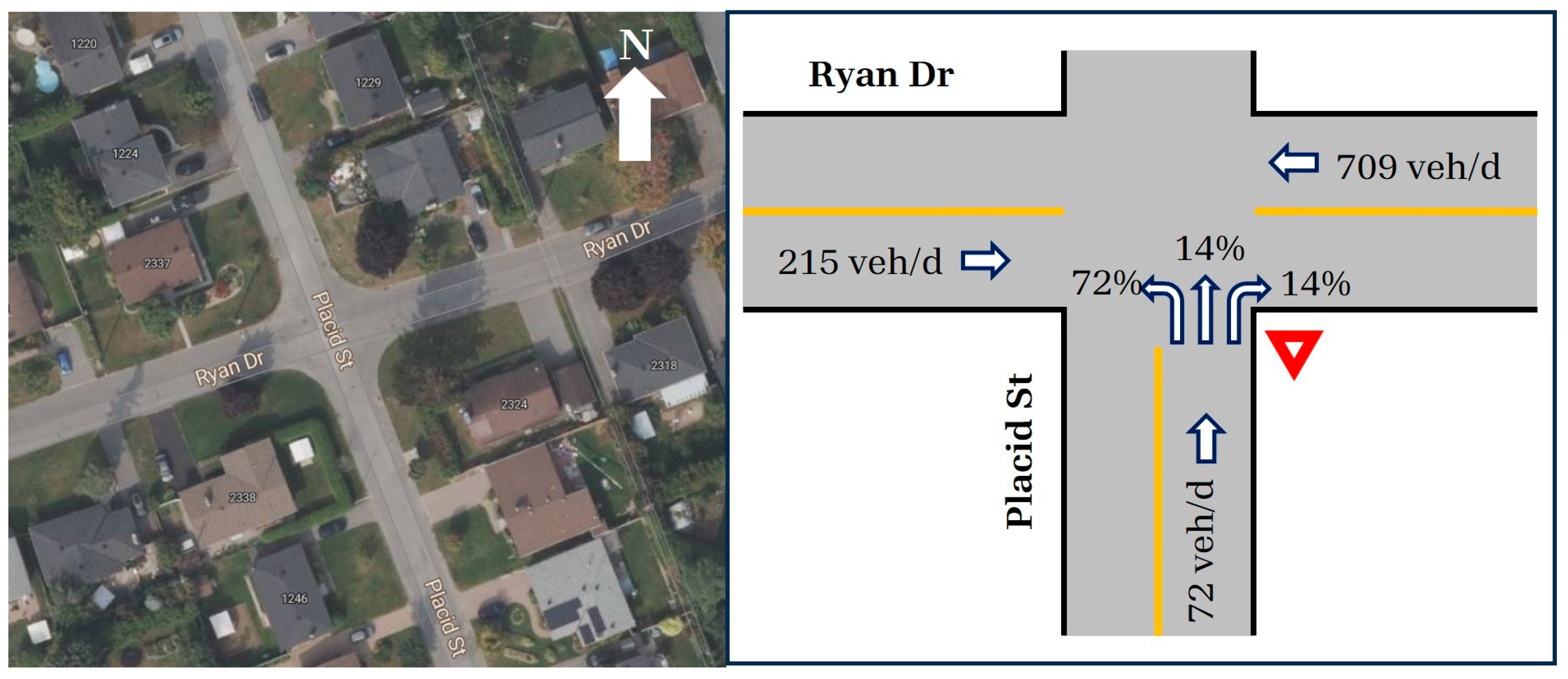
Correlation among the driving behaviors of AVs is not expected since these vehicles will follow computerized logic. Therefore, the potential correlations among driving behavior-based variables such as traveling speeds, reaction times, deceleration/acceleration, turning speeds, vehicle positions within the lane, accepted time gaps, and time headway were investigated only for DVs. However, the literature showed little or no correlation among these variables. Several studies showed low correlations among deceleration, traveling speed, and PRT [32,33,34]. Intuitively, the turning speed and vehicle position within the lane have relationships with the effective turning radius and lane width, respectively. However, in studying a specific intersection, the lane width is fixed, and the effective turning radius is almost constant. Subsequently, correlation is not relevant. Also, several studies have suggested that the time headway variable is constant over various speeds [35,36,37]. According to the Green Book [1], the accepted time gaps increase with the number of lanes, roadway grades, or vehicle type. However, these parameters are fixed parameters for a specific study intersection. Also, no relationship between driver behavior and the vehicle-related distance variables was considered since the latter was based on the design of the vehicle. As a result, correlations were not considered in this study.

4. Case Study

A yield-controlled urban intersection between Ryan Drive (major road) and Placid Street (minor road) in Ottawa, Ontario, was selected as a case study intersection to illustrate the application of the developed methodology. The intersection’s latitude and longitude are (45.3481, −75.7783). As per the general characteristics assumed in the developed model, the intersection is four-legged, right-angle, and both intersecting roads are two-lane and undivided. Only the north-bound (NB) approach on Placid Street is analyzed in this case study, where sight obstructions are observed on both sides. Site-specific geometric data were collected as follows:

• Lane width (both roads): 3.6 m.
• Speed limit (both roads): 40 km/h. The design speed of both roads was assumed as 50 km/h or 10 km/h above the speed limit.
• Curb radius: 7.5 m.
• Road shoulders: none.

The effective turning radius ($R_t$) for right and left turns was estimated based on the intersection geometry. For right turns, $R_t$ was taken as the curb radius plus a 0.5 lane width, resulting in a value of 9.3 m. For left turns, $R_t$ was assumed equal to curb radius plus a 1.5 lane width, yielding $R_t$ of 12.9 m. The peak-hour traffic volume (PHV) and the volume of each maneuver type were obtained for this intersection from video recordings supplied by the City of Ottawa. The City of Ottawa’s peak-hour expansion factor was applied to estimate the average daily traffic (ADT). The resulting ADT data are represented along with the general intersection layout in Figure 9.

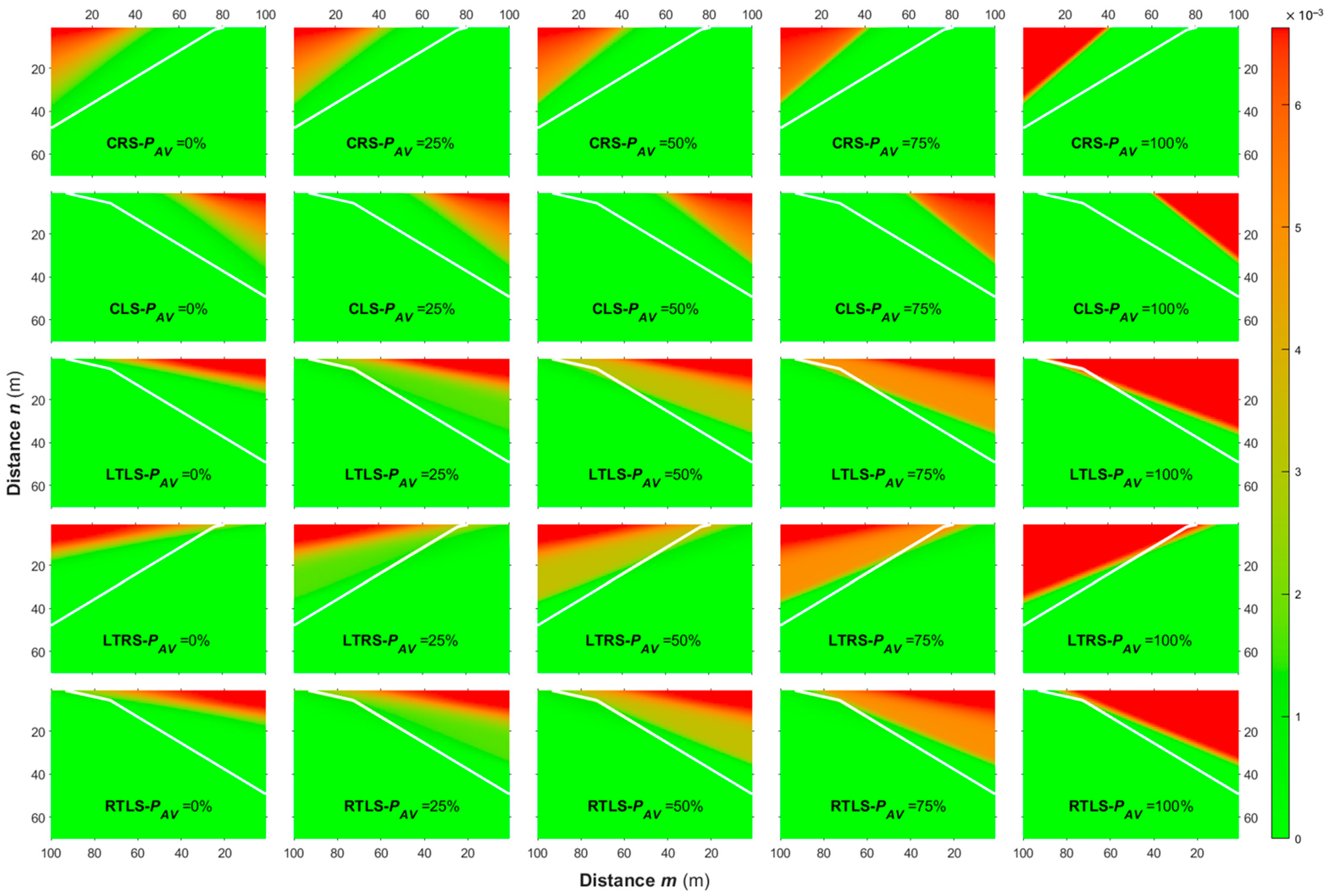
4.1. Results of Conflict Analysis

Using Equation (1), the conflict frequency was estimated for each vehicle interaction and conflict type at five AV penetration rates ($P_{AV}$) ranging from 0% (DV-only traffic) to 100% (AV-only traffic). Mixed traffic was considered for the $P_{AV}$ values of 25, 50, and 75%. As mentioned earlier, all the daily traffic is assumed to arrive within an 18 h period and a conflict is assumed to take place if the minor vehicle arrives within 2 s of the arrival of a major-road vehicle. Subsequently,

Table 5. Average number of daily conflicts at study intersection.

Interaction Type	PAV (%)	CRS	CLS	LTLS	LTRS	RTLS
	0	0.2188	0.0663	0.3445	1.1361	0.0663
	25	0.1231	0.0373	0.1939	0.6393	0.0373
DVN-DVM	50	0.0547	0.0166	0.0862	0.2842	0.0166
	75	0.0137	0.0041	0.0216	0.0711	0.0041
	100	0	0	0	0	0
	0	0	0	0	0	0
	25	0.0410	0.0124	0.0647	0.2133	0.0124
DVN-AVM	50	0.0547	0.0166	0.0862	0.2842	0.0166
	75	0.0410	0.0124	0.0646	0.2131	0.0124
	100	0	0	0	0	0
	0	0	0	0	0	0
	25	0.0410	0.0124	0.0646	0.2131	0.0124
AVN-DVM	50	0.0547	0.0166	0.0862	0.2842	0.0166
	75	0.0410	0.0124	0.0647	0.2133	0.0124
	100	0	0	0	0	0
	0	0	0	0	0	0
	25	0.0137	0.0041	0.0216	0.0711	0.0041
AVN-AVM	50	0.0547	0.0166	0.0862	0.2842	0.0166
	75	0.1231	0.0373	0.1939	0.6393	0.0373
	100	0.2188	0.0663	0.3445	1.1361	0.0663

shows the average number of daily conflicts on the study intersection for four vehicle interaction types, five $P_{AV}$ rates, and five conflict types.

4.2. PUC Results

A Matlab script was developed to apply the developed procedure to yield controlled intersections and was applied to the study intersection. The number of simulations was originally set at 200,000 vehicles of each type on each road. However, the generated vehicle parameters were checked for outliers using the quartile method to exclude vehicle parameter combinations that can produce unreasonable ISD values. In this method, an interquartile range (IQR) is calculated as the difference between the third quartile (Q3 or 75th percentile in the cumulative frequency distribution) and the first quartile (Q1 or 25th percentile). Outliers are then identified as those elements that are greater than Q3 + 1.5IQR or less than Q1 = 1.5IQR. Furthermore, after calculating the ISD on minor and major roads, the potential ISD outliers were removed using the Grubbs method [38], which checks extreme data one by one. Ultimately, just over 150,000 vehicles of each type on each road were used in the analysis.

4.2.1. Target PUC

To estimate the target PUC for the study intersection, the Green Book criteria were applied as explained in Section 2.7. For a minor-road speed limit of 40 km/h (design speed assumed as 50 km/h), Table 2 shows that for the crossing maneuver, $S_N$ = 55 m and $t_g$ = 6.5 s leading to $S_M$ = 90.3 m. As mentioned earlier, for turning maneuvers the Green Book recommends $S_N$ = 25 m and $t_g$ = 8.0 s leading to $S_M$ = 111.1 m. Using these values and following the methodology in Section 2.7, the maximum PUC for both the right- and left-side conflicts corresponded to the location with the lowest $n$ and $n^{\prime }$ values. Specifically, the maximum right-side PUC (combining the CRS and LTRS normalized over the sum of the minor road’s through and left-turn volumes) was 7.43 × 10⁻³ with the object located at $m$ = 85 m and $n$ = 0.07 m. The maximum left-side PUC (combining the CLS, LTLS, and RTLS normalized over the minor road’s total approach volume) was 0.34 × 10⁻³ with the object located at $m^{\prime }$ = 97 m and $n^{\prime }$= 0.16 m. Combining these two PUC values, the target PUC (normalized over the minor road’s total approach volume) was 6.74 × 10⁻³.

4.2.2. Effect of AVs

To visualize the change in the PUC with $P_{AV}$, the PUC was estimated for a fine mesh of 7000 possible object locations at the study intersection ($m$, $m^{\prime }$ = [1, 100] m, and $n$, $n^{\prime }$ = [1, 70] m) and the five different PAV rates. Figure 10 illustrates the change in the PUC with object location using a heatmap for each conflict type and PAV rate. The figure also shows the AASHTO sight line overlapped with each heatmap. As mentioned earlier and as shown in the figure, the AASHTO sight line is actually a broken line as it combines the two limiting lines corresponding to crossing and turning maneuvers as explained in Section 2.7.

The color scale clearly shows that all the conflicts experience an increase in the PUC as $P_{AV}$ increases. The main contributing factors to this trend are related to the driving logic assumed for AVs. First, the assumption that AVs would reduce crossing speed only if a conflict is perceived causes the AV’s ISD on the minor road to be higher than the DV’s. By comparing the speed distributions of minor-road vehicles in Figure 11a, AVs stick more closely to the speed limit and hence have lower midblock speeds than those of DVs. However, DVs’ crossing speeds ($v_{c,DV}$) are mostly lower than the AVs’ midblock speeds. Subsequently, Figure 11b shows that most of the distribution of the minor-road-crossing ISD for DVs ($S_{N,DV-C}$) is lower than that for AVs ($S_{N,AV}$). In addition, AVs were assumed to utilize lower mean braking rates due to the disengagement of the vehicle occupants from the driving task and the higher discomfort expected at high braking rates. The result is a much lower ISD for turning DVs ($S_{N,DV-T}$) than for turning AVs as shown in the distributions in Figure 11b. Finally, the distributions of $t_g$ for all the turning conflicts show that AVs require higher $t_g$ values than those of DVs, especially for the LTLS. The main reason again is the AVs’ lower braking rate, which causes the AVs to decide to stop or proceed through the intersection at the full stopping sight distance before the intersection. It should be noted, however, that major-road AVs also stick to the speed limit more closely than DVs. Subsequently, as per Equation (10), the increase in $t_g$ associated with Avs that should produce a less pronounced increase in $S_M$.

It is worth noting that the AASHTO ISD for crossing and turning are overlapped in Figure 11b as vertical lines after correcting them to correspond to the distance from the edge of the road. The figure clearly shows that AASHTO’s ISD corresponds to a very high percentile in the DV_N’s ISD distribution. The same observation can be noted for AASHTO’s $t_g$ values in Figure 11c–f. These observations reflect the conservative nature of the deterministic design in the Green Book [1].

The object locations corresponding to the maximum right- and left-side PUC values in the target PUC analysis were assumed as the object locations for mixed traffic. That is, a right-side object was assumed at $m$ = 85 m and $n$ = 0.07 m, and a left-side object was assumed at $m^{\prime }$ = 97 m and $n^{\prime }$ = 0.16 m. The resulting overall PUC values, denoted as “Original PUC” in

Table 6. PUC values for mixed vehicle fleets.

PAV	Original PUC	Reduced AV Speed Limit (km/h)	Reduced PUC
25	7.89 × 10−3	36	6.62 × 10−3
50	9.53 × 10−3	36	5.93 × 10−3
75	1.17 × 10−2	37	6.44 × 10−3
100	1.43 × 10−2	37	5.73 × 10−3

, show that the intersection would experience an overall PUC that is higher than the target value in the mixed vehicle and AV-only environments ($P_{AV}$ > 0). A possible remedy to reduce these PUC values such that they do not exceed the target PUC is to reduce the AV speed limit on the minor-road approach to the yield control. This measure is equivalent to the speed reduction observed for DVs as they approach the yield control as mentioned earlier. The PUC was recalculated for the mixed vehicle and AV-only environments through iterations involving reducing the AV speed limit on the minor road at a 1 km/h step while keeping all the other speed limits fixed. As shown in Table 6, the reduced AV speed limit on the minor road ranged from 36 to 37 km/h.

Interestingly, the lowest minor-road AV speed limit is required at the lower $P_{AV}$ rates from 25 to 50%. To understand this finding, the change in the PUC for individual conflicts and all right and left SDTs was plotted against the object distance $m$ (or $m^{\prime }$) for a fixed object distance $n$ (or $n^{\prime }$) of 1.0 m (see Figure 12). This 1.0 m distance for $n$ and $n^{\prime }$ is the closest value to the assumed object location. The figure also shows the object locations m and m’ that correspond to the object location corresponding to the target PUC. As shown in the figure, the individual and combined PUC values for DV-only traffic ($P_{AV}$ = 0) decrease gradually as $m$ (or $m^{\prime }$) increases. On the other hand, as $P_{AV}$ increases, abrupt PUC reductions become more visible. For example, for AV-only traffic ($P_{AV}$ = 100%), each individual PUC is almost fixed for low values of $m$ (or $m^{\prime }$) and then diminishes quickly after a specific object location. The likely reason for this high rate of reduction is the narrow distributions of all the AV parameters, which reduce variability in the ISD requirements. In addition, since crossing conflicts’ PUCs diminish at lower values of $m$ (or $m^{\prime }$) compared to those of turning conflicts, the combined PUCs tend to have a cyclic pattern of fixed values followed by an abrupt reduction. The figures also show that before the abrupt PUC reduction, the PUC is higher for the higher $P_{AV}$ rates, but an opposite trend is evident after the midpoint of the abrupt PUC reduction.

5. Concluding Remarks

This study investigated intersection sight distance (ISD) requirements at intersections with yield control on a minor road. This paper also covered conventional, driver-operated vehicles (DVs) and automated vehicles (AVs). After elaborating on the potential conflict types that can develop at yield-controlled intersections, a detailed procedure and models were developed to estimate the number of conflicts and ISD requirements for each combination of conflict and vehicle interaction types. A reliability-based surrogate safety measure, referred to as the probability of unresolved conflicts (PUC), was developed to reflect the probability of minor-road vehicles experiencing a demand ISD greater than the available ISD while involved in a conflict with major-road vehicles. As a relationship between the PUC and objective safety performance is not available yet, a procedure was developed to compare the PUC in a mixed or AV-only environment to a target PUC value, which corresponds to the maximum expected PUC if the ISD is compliant with the Green Book requirements. Variation in the DV and AV parameters that can affect ISD was considered, and the distribution of each parameter was sourced from the literature or collected data. The developed models were applied using Monte Carlo Simulation (MCS) to a case study of a yield-controlled intersection in Ottawa, Ontario.

The analysis of the ISD at the study intersection showed that the PUC generally increases as the AV penetration rate increases. Factors contributing to this increase are mainly related to AV driving logic and parameters. In mixed and AV-only environments, an object that does not obstruct the ISD according to the Green Book guidelines can produce PUC values that are higher than the target PUC value. Thus, the intersection may exhibit a lower safety performance with the adoption of AVs in the vehicle fleet. A potential measure to correct this problem is to reduce AV speeds as they approach a yield-controlled intersection. Such a feat can be attained by having AV-specific speed limit signs along roadways. Alternatively, decreased speeds for AVs can be achieved through the use of smart technologies such as speed assist systems as they approach a yield-controlled intersection. Speed assist systems select a vehicle speed for an AV from a speed limit map database [39].

It is noted, however, that the Green Book ISD guidelines are based on a deterministic approach where a near-worst-case value is assumed for each design parameter. This approach can lead to a conservative design, which was evident in comparing the ISD recommendations to the distribution of ISD requirements for the study intersection. It is therefore likely that a target PUC value less than the value proposed in this paper can lead to acceptable ISD criteria. A dataset of yield-controlled intersections with known geometry and collision experience can be used to establish a relationship between the collision frequency and the PUC. Such a relationship would allow designers to explicitly assess the consequences of their design on safety performance. It is recommended that the methodology demonstrated is modified and used in exploring the safety implications of a mixed vehicle fleet on the ISD at intersections with other types of control such as stop-controlled intersections.

References

1. AASHTO. A Policy on Geometric Design of Highway and Streets, 7th ed.; The American Association of State Highway and Transportation Officials: Washington, DC, USA, 2018. [Google Scholar]
2. TAC. Geometric Design Guide for Canadian Roads; Technical Report; Transportation Association of Canada: Ottawa, ON, Canada, 2017. [Google Scholar]
3. Harwood, D.; Mason, J.; Brydia, R.; Pietrucha, M.; Gittings, G. Report 383: Intersection Sight Distance; Transportation Research Board (TRB): Washington, DC, USA, 1996. [Google Scholar]
4. Easa, S.M. Reliability Approach to Intersection Sight Distance Design. Transp. Res. Rec. 2000, 1701, 42–52. [Google Scholar] [CrossRef]
5. Easa, S.M.; Ma, Y.; Liu, S.; Yang, Y.; Arkatkar, S. Reliability Analysis of Intersection Sight Distance at Roundabouts. Infrastructures 2020, 5, 67. [Google Scholar] [CrossRef]
6. Easa, S.M.; Hussain, A. Reliability of Sight Distance at Stop-Control Intersections. Proc. Inst. Civ. Eng.—Transp. 2016, 169, 138–147. [Google Scholar] [CrossRef]
7. Hussain, A.; Easa, S.M. Reliability Analysis of Left-Turn Sight Distance at Signalized Intersections. J. Transp. Eng. 2016, 142, 04015048. [Google Scholar] [CrossRef]
8. Osama, A.; Sayed, T.; Easa, S. Framework for Evaluating Risk of Limited Sight Distance for Permitted Left-Turn Movements: Case Study. Can. J. Civ. Eng. 2016, 43, 369–377. [Google Scholar] [CrossRef]
9. Sarran, S.; Hassan, Y. Impacts of Automated Vehicles in a Mixed Environment on Intersection Sight Distance at Uncontrolled Intersections. J. Transp. Eng. A Syst. 2025, 151, 04024016. [Google Scholar] [CrossRef]
10. Rengaraju, V.R.; Rao, V.T. Vehicle-Arrival Characteristics at Urban Uncontrolled Intersections. J. Transp. Eng. 1995, 121, 317–323. [Google Scholar] [CrossRef]
11. Yin, W.; Zou, Q.; Lv, C.; Wu, Z.; Tan, G. A Quantitative Model of Conflict Risk Degree at Non-Signalized Intersections. Procedia Eng. 2016, 137, 171–179. [Google Scholar] [CrossRef]
12. MathWorks, R2024b, Triangular Distribution—MATLAB & Simulink; MathWork: Natick, MA, USA, 2024. Available online: https://www.mathworks.com/help/stats/triangular-distribution.html (accessed on 4 April 2024).
13. Dabbour, E. Design Gap Acceptance for Right-Turning Vehicles Based on Vehicle Acceleration Capabilities. Transp. Res. Record. 2015, 2521, 12–21. [Google Scholar] [CrossRef]
14. Dabbour, E.; Easa, S. Sight-Distance Requirements for Left-Turning Vehicles at Two-Way Stop-Controlled Intersections. J. Transp. Eng. Part A Syst. 2017, 143, 04016004. [Google Scholar] [CrossRef]
15. Abdelnaby, A.; Hassan, Y. Probabilistic Analysis of Freeway Deceleration Speed-Change Lanes. Transp. Res. Rec. 2014, 2404, 27–37. [Google Scholar] [CrossRef]
16. Huang, C.; El Hami, A.; Radi, B. Overview of structural reliability analysis methods—Part I: Local reliability methods. Incertitudes et fiabilité des systèmes multiphysiques. Engineering 2017, 17, 1–10. [Google Scholar] [CrossRef]
17. Andrade-Catano, F.; De Santos-Berbel, C.; Castro, M. Reliability-Based Safety Evaluation of Headlight Sight Distance Applied to Road Sag Curve Standards. IEEE Access 2020, 8, 43606–43617. [Google Scholar] [CrossRef]
18. Singh, V.P.; Jain, S.K.; Tyagi, A. Risk and Reliability Analysis: A Handbook for Civil and Environmental Engineers; American Society of Civil Engineers: Reston, VA, USA, 2007. [Google Scholar] [CrossRef]
19. Sarhan, M.; Hassan, Y. Three-dimensional, Probabilistic Highway Design: Sight Distance Application. Transp. Res. Rec. 2008, 2060, 10–18. [Google Scholar] [CrossRef]
20. Akaike, H. A New Look at the Statistical Model Identification. IEEE Trans. Autom. Control 1974, 19, 716–723. [Google Scholar] [CrossRef]
21. Stone, M. Comments on Model Selection Criteria of Akaike and Schwartz. J. R. Stat. Soc. B 1979, 41, 276–278. [Google Scholar] [CrossRef]
22. Kuha, J. AIC and BIC: Comparisons of Assumptions and Performance. Sociol. Methods Res. 2004, 33, 188–229. [Google Scholar] [CrossRef]
23. Sukennik, P. Deliverable 2.5: Microsimulation Guide for Automated Vehicles; Technical Report. CoEXist; PTV Group: Karlsruhe, Germany, 2018. [Google Scholar]
24. Fambro, D.; Fitzpatrick, K.; Koppa, R. National Cooperative Highway Research Program Report (NCHRP) 400: Determination of Stopping Sight Distances; Transportation Research Board (TRB): Washington, DC, USA, 1997. [Google Scholar]
25. Peng, H. Driving Etiquette; Technical Report; Transportation Research Institute: Ann Arbor, MI, USA, 2020. [Google Scholar]
26. Ismail, K.; Sayed, T. Risk-Based Framework for Accommodating Uncertainty in Highway Geometric Design. Can. J. Civ. Eng. 2009, 36, 743–753. [Google Scholar] [CrossRef]
27. Moon, S.; Yi, K. Human Driving Data-Based Design of a Vehicle Adaptive Cruise Control Algorithm. Veh. Syst. Dyn. 2008, 46, 661–690. [Google Scholar] [CrossRef]
28. Urmson, C. Driving Beyond Stopping Distance Constraints. In Proceedings of the 2006 IEEE/RSJ International Conference on Intelligent Robots and Systems, Beijing, China, 9–15 October 2006; pp. 1189–1194. [Google Scholar] [CrossRef]
29. Sukennik, P.; Kautzsch, L. Deliverable 2.3: Default Behavioral Parameter Sets for Automated Vehicles (AV). CoEXist; PTV Group: Karlsruhe, Germany, 2018. [Google Scholar]
30. Weber, Y.; Kanarachos, S. CUPAC—The Coventry University public road dataset for automated cars. Data Brief 2020, 28, 104950. [Google Scholar] [CrossRef]
31. Tesla. Model 3 Owner’s Manual: About Auto Pilot; Tesla, Inc.: Austin, TX, USA, 2025. [Google Scholar]
32. Wortman, R.H.; Matthias, J.S. An Evaluation of Driver Behavior at Signalized Intersections. Transp. Res. Rec. 1983, 904, 10–20. [Google Scholar]
33. Wang, J.; Dixon, K.K.; Li, H.; Ogle, J. Normal Acceleration Behavior of Passenger Vehicles Starting from Rest at All-Way Stop-Controlled Intersections. Transp. Res. Rec. 2004, 1883, 158–166. [Google Scholar] [CrossRef]
34. Wood, J.S.; Zhang, S. Evaluating Relationships Between Perception-Reaction Times, Emergency Deceleration Rates, and Crash Outcomes Using Naturalistic Driving Data. Transp. Res. Rec. 2021, 2675, 213–223. [Google Scholar] [CrossRef]
35. Siebert, F.W.; Oehl, M.; Pfister, H.R. The Influence of Time Headway on Subjective Driver States in Adaptive Cruise Control. Transp. Res. Part F Traffic Psychol. Behav. 2014, 25, 65–73. [Google Scholar] [CrossRef]
36. Siebert, F.W.; Oehl, M.; Bersch, F.; Pfister, H.R. The Exact Determination of Subjective Risk and Comfort Thresholds in Car Following. Transp. Res. Part F Traffic Psychol. Behav. 2017, 46, 1–13. [Google Scholar] [CrossRef]
37. Winsum, W.V.; Heino, A. Choice of Time-Headway in Car-Following and the Role of Time-to-Collision Information in Braking. Ergonomic 1996, 39, 579–592. [Google Scholar] [CrossRef]
38. Grubbs, F.E. Procedures for Detecting Outlying Observations in Samples. Technometrics 1969, 11, 1–21. [Google Scholar] [CrossRef]
39. Demuynck, V. Driving Safely with ADAS Map Speed Limits. TomTom 2020. Available online: https://www.tomtom.com/newsroom/product-focus/adas-map-speed-limits/ (accessed on 18 March 2025).
Figure 1. Study methodological framework.
Smartcities 08 00073 g001
Figure 2. Possible interactions between minor- and major-road vehicles.
Smartcities 08 00073 g002
Figure 3. Typical right- and left-side SDTs.
Smartcities 08 00073 g003
Figure 4. Speed profiles of minor-road DVs at a yield-controlled intersection.
Smartcities 08 00073 g004
Figure 5. Estimating t g for crossing conflicts (CRS and CLS).
Smartcities 08 00073 g005
Figure 6. Estimating t g for LTLS conflict.
Smartcities 08 00073 g006
Figure 7. Estimating t g for LTRS and RTLS conflict.
Smartcities 08 00073 g007
Figure 8. Modeling sight line for the green book guidelines.
Smartcities 08 00073 g008
Figure 9. Layout of study intersection (source of satellite image: Bing Maps).
Smartcities 08 00073 g009
Figure 10. PUC Results for Different Object Locations and P A V Rates.
Smartcities 08 00073 g010
Figure 11. Distribution of vehicle speeds and ISD parameters in MCS.
Smartcities 08 00073 g011
Figure 12. Change in PUC with object location and P A V .
Smartcities 08 00073 g012