Abstract
This paper deals with the problem of predetermining the spray angle and uniformity of the flat fan sprayer with a semicircular impact surface for the intra-soil application of liquid mineral fertilizers. The jet impact on a round splash plate and radial atomization properties are investigated theoretically, the formation features of the spray with an obtuse angle are studied in a geometrical way, and the design search of the nozzle shape and optimization calculations are performed using computational fluid dynamics (CFD) simulations and then verified experimentally. It was revealed that the spray rate and spray angle can be adjusted by changing the parameter s, and when the spray angle is within s = 0–0.2 mm, it forms spray angles with range of 140°–175°. The spraying angle, in turn, shows the potential length of the tillage knife in accordance with the undersoil cavity dimensions. A spray uniformity of up to 74% was achieved, which is sufficient for applied studies and for intra-soil application operations. According to the investigations and field experiments, it can be concluded that the designed nozzle is applicable for the intra-soil application of liquid mineral fertilizers. The use of flat fan nozzles that form a spraying band under the soil cavity and along the entire length of the tillage knife ensures a highly efficient mixing process, the liquid mineral fertilizers with treated soil (particles) positively contributing to plant maturation.
1. Introduction
The reduction of soil fertility is one of the main problems in Kazakhstan’s agriculture, and the problem occurs in many other countries engaged in agriculture, especially in crop production [1,2,3,4,5].
One of the approaches to solving the problem is the implementation of systematic measures for soil cultivation, the introduction of ameliorants, aimed at preserving the moisture, mineral, and nutrient substances of arable land, to create favorable conditions for the development of a stable root system of plants [6].
The intra-soil application of fertilizers is an effective way to exact the placement of necessary doses of nutritious elements at required soil depths concerning the soil condition and using differential application technology [7]. Intra-soil application can reduce various losses such volatilization, leaching, surface runoff, and denitrification from the soil–plant system [8].
Liquid mineral fertilizers (LMFs) are more manageable, and the absorption of fertilizer by plant roots happens better; it prevents roots from floating, enhancing the lodging resistance of crops [9]. The effect of liquid mineral fertilizers comes faster, evenly assimilated, and has a long-lasting effect [10]. An important advantage of liquid forms of mineral fertilizers is the low cost [11] of their storage, transportation, and application, and LMFs can be metered out precisely and handled easily [12]. The application of liquid fertilizers simultaneously with sowing allows to reduce the number of equipment passes and saves fuel [13] and work time; the accuracy of the application saves the LMFs.
Several types of nozzles are available for agricultural spraying for pesticide or mineral and nutrient substance application, and each nozzle has a function and purpose. The primary function of nozzles is breaking the liquid under pressurized spray into droplets with a wide range of droplet sizes [14,15,16,17]. The quality of agricultural spraying largely depends on the uniformity of the distribution of the sprayed liquid over the spraying surface [18]. However, all the investigated nozzles are mainly designed for the surface application of ameliorants.
In the research, a universal deep loosener fertilizer for the intra-soil application of granular and liquid mineral fertilizers was proposed. As an executive part of the agricultural unit, a flat fan nozzle that allows introducing the liquid fertilizers under the soil to the plant roots developing area was designed [19]. The nozzles are designed with low height parameters, because they can negatively influence the draft force of the agricultural unit [19,20,21]. In turn, they must provide the required spraying angle and width of the treated strip. In previous studies, the form and parameters of the suggested nozzle have been analyzed [22]. However, research on the problems of spray uniformity, perpendicularity (symmetry), and atomization angle of flat fan atomizers with a semicircular impact surface are still ongoing, so this paper focused on these problems. The main scientific questions that relate to the nozzle parameterization are on atomization or spraying processes that connect with the fluid dynamics and geometrical features of the nozzle.
The process of atomization often involves ejecting thin liquid sheets at high velocities from a nozzle, which causes the sheet to break up into fine droplets, and if the jet impacts on a round splash plate, it forms a round sheet [23]. A fundamental classification of atomization processes, where jets impacting circular splash plates are described as a liquid breakup method that works without air pressure, was presented in [24]. A complete analysis of the radial spread of a liquid jet over a horizontal plane was performed by [25] using the boundary layer theory. In his investigations, the film motion and liquid sheet forming process was investigated analytically by considering the flow dynamics in four separate regions. Wu et al. (2007) used a free surface impinging jet theory to determine the liquid film thickness and velocity at the edge of the deflector [26]. The fluid flow and atomization conditions (flag regime, sheet thickness, wavelength, etc.) related to radially expanding liquid sheets and the breakup proses into droplets was studied in [27]. In their study, the entire period of liquid sheet was covered, considering the dynamics of its formation and destruction, as well as the stationary regime in which the transition from sheet to drops occurs. Most theoretical studies of jet nozzles are devoted to sprayers with a cylindrical nozzle [28], and a mathematical model that primary describes the flow through the nozzle with a semicircle impact surface has not been developed yet.
During the study, existing flat fan spray nozzles [29,30] and their suitability with the hypothesis of the study were evaluated by visual analysis using CFD simulations. The main disadvantages of the existing atomizers are design complexity (two or more components), high cost, and small spray angle; many existing flat fan nozzles are not directed to apply liquid mineral fertilizers (LMFs) to the soil.
The film thickness [31] and the velocity [32] are governing parameters of such flat fan spray formation processes and for applied investigations. In our case, the impact surface of the proposed nozzle has a semicircular shape and provides the formation of the required spray angle to ensure the treated (moistened) strip (band) in the subsoil cavity along the trail of a tillage knife [33].
The main objective of this work is to investigate the initial theoretical basics of the flow through the designed nozzle with a semicircle impact surface and determine the parameters and their limits, which have an influence on the spray angle and uniformity [14,15]. For this purpose, the theories of a radial spread liquid jet over a horizontal round plate were studied, existing equations were analyzed, and nozzle parameters were optimized using Ansys Fluent®. The performance of the nozzles was experimentally verified. Sufficient spray uniformity was achieved through optimization calculations using CFD tools, verified experimentally using a measuring vessel, and further investigated in a laboratory soil bin by mounting the nozzle on a tillage knife and moving at a low speed.
2. Materials and Methods
2.1. Nozzle Design
The spraying nozzle installed on the flat cutting knives of the universal deep loosener fertilizer working organ has a semicircular impact surface where the jet is perpendicular on it. The nozzle design and important parameters are given in [21]. The scheme of the presented spray nozzle is shown in Figure 1. The spray nozzle consists of horizontal and vertical cylindrical feed channels (d and d1, respectively) and an impact surface DS (deflector) that has a common center with the vertical feed channel. The main part of the nozzle is the orifice with a height (h) that allows a wide, flat, arc-shaped flow. α1 is the spray guiding angle, s is the distance from the center of the impact surface to the chord of the semicircle (wall), and K is the distance between the impact surface and the axis of the horizontal delivery channel. β and γ are the fall angles that indicate the upward and downward deviations of the flow relative to the horizontal plane. The velocity of the fluid in the vertical channel is Vj, and the outlet velocity (as a thin stream) is Vo.
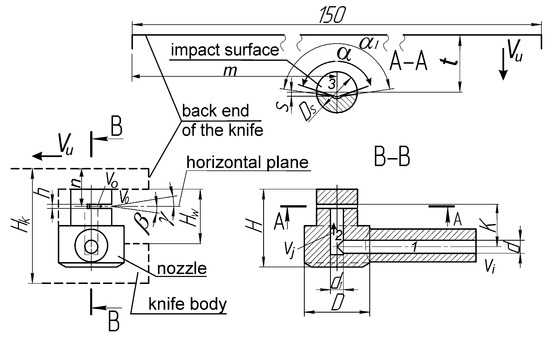
Figure 1.
Scheme of a flat fan sprayer with a semicircular impact surface.
Although the flow in the horizontal delivery channel (1) is laminar, the bi-level and mutual perpendicularity of the inlet and outlet (3) flow directions (intersection of the flows) form a turbulent flow. Accordingly, K is the distance between these two flow directions that forms the vertical feed (2) channel connecting the feed and spray orifices, which is important to decrease the turbulent flow; however, it is impossible to lengthen according to the given height of the knife.
The nozzle can be mounted on the knife in positions where the atomization orifice (slot) may be located in slot-up or slot-down positions in relation to the axis of the feed channel. However, it depends on the spray fall angle.
It is believed that the slot height h, fluid delivery diameter d1, and distance s provides the necessary uniform atomization with an obtuse angle. The spray guide angle α1 ensures the required spray angle (α). The atomization angle is an important resultant parameter that indicates the suitability of the nozzle. It provides a 150 mm wide liquid strip along the knife trail.
The sprayer can be suitable for surface application, as well as for use with a plow point and in other areas of industry such as air humidification, fire prevention, etc.
2.2. Theoretical Analyses
If the density or viscosity of the fluid is not taken into account, the spray angle of a flat atomizer with a semicircular impact surface can be expressed by the length of the edge washed by the liquid flow on its impact surface. The diameter (d1) of the vertical feed channel and the height of the radial orifice (h) determine the flow area, where the flow passes from the vertical channel to the horizontal spray slot. This orifice can be called the flow transition window. Figure 2 shows the formation of the flow scheme on the impact surface and atomization angle.
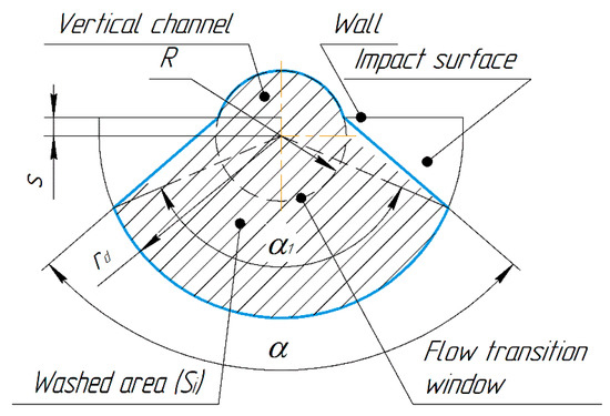
Figure 2.
Scheme of spray angle formation on the impact surface of the chosen orifice shape.
The volume of liquid flowing out of the transition window (Qtr) during a certain period is expressed by the following formula:
where Vtr is the flow velocity at the transition window, and Atr is the area of the transition window. In real conditions, the volume of fluid flowing out the slot (in spray or sheet form) depends on how much fluid fills the slot surface and obtains flow thickness. This liquid volume (Equation (2)) covers and washes the impact surface (Si) after a certain time and then tends outward:
where Qi is the volume of liquid that washes the impact surface, and hd is the average thickness of the flow formed at the impact surface.
Consequently, the formed spray angle will depend on the hd and fluid flow rate over the impact surface. Indeed, Vtr > Vo; however, if the radius rd is very low, it can be nearly equal. Accordingly, the volume of liquid flowing out Qo of the outer orifice opening is also expressed using the following formula:
where Vo is the outlet velocity, and Ao is the area of the outlet slot.
Consequently, the outlet area is Ao = hd πrd, and here, πrd should be replaced by the actual arc edge (Lo). The Lo, in turn, depends on how much the liquid overflows on the impact surface. Geometrically, Lo is associated with the actual spray angle α.
The definition of the arc length of a semicircle is known, and the total arc length, which is formed with the addition of the parameter s, is equal to the sum of the doubled angle α and 180°. according to the Pythagoras theorem, is defined as follows:
where R is the semicircle radius or radius of the vertical delivery channel, and s is the distance from the center of the impact surface. Geometrically, it is known that the length of a sector arc L is determined by the following formula:
where α is an actual angular value.
Based on the ratio of s to R, the value of α is determined using the Bradis table. For our case, the formula is transformed as follows:
Analyses show that the hd is mostly independent of h, and it is problematic to convert the actual angle value to a numerical value when working with CFD tools, which is a notable disadvantage of Equation (6). Therefore, here subsists another parameter affecting the flow domain, and another way of determining the arc length has to be considered that would define the spray angle.
As can be seen from Figure 3, the change in the size of the washed area is influenced by the parameter s, which determines the position of the rear wall of the opening in the transition area. Here, 1 is the area where a real powerful liquid flow occurs and 2 an area in which a free or turbulent liquid flow is formed; sometimes, it can be empty. It turns out that the formation of the spray angle is also directly influenced by the parameter s along with the inlet velocity, and it contributes to the formation of a strong pressure on the impact surface.
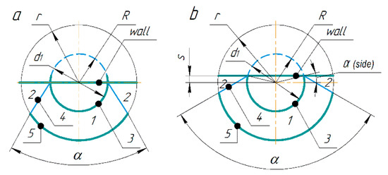
Figure 3.
Possible atomization angle on the impact surface when s = 0 (a) and s > 0 (b).
Line 4 between zones 1 and 2 can form a future spraying angle. Line 3 is the edge of the vertical feed channel, and its arc length (Ltr) determines the flow transition window area. Figure 3 also shows the formation of the angle α in the cases when s = 0 (a) and s > 0 (b). A strong outlet washing arc 5 (Lo) on the impact surface helps to determine the spray angle.
The area of the transition window from the vertical feed channel to the horizontal spray slot is determined by the equality below:
If considering the determination of the arc length by the height (here, conventionally marked with h) of a segment that is formed with respect to the s parameter (Figure 4), it is known that the area of the transition window is defined by Equation (7), and here, and this, in turn, will be .
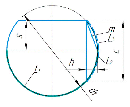
Figure 4.
Scheme for determining the arc length (Ltr) by segment height.
As can be seen from the scheme, if we consider the parameter s as a chord, the arc length can be defined by the following formula:
where m is the hypotenuse that is defined by s and h. Additionally, it can be a chord of arc L3. It is known that , c = 2s.
Based on this, the formula for determining the arc length over the chord corresponding to our case will look as follows:
or
Then, the formula for determining the total arc length is defined as
The value of m is defined according to the Pythagoras theorem:
where, h is the height of the segment. The formula for its definition is known:
As c = 2s, Equation (13) is converted as follows:
After simplifying,
Due to the multiplier decomposition and simplifying, the formula for determining the value is represented as follows:
Defined Equations (11) and (17) are the basic formulas and are suitable for use in CFD calculations to obtain the reported results. Based on the above, the following formula for determining the arc length at the exit edge of the atomizer is suggested:
where hdt is the thickness of the flow in the transition window, and hd is the thickness of the flow on the impact surface. The hd for a nozzle with a semicircle shape can be defined as
However, Equations (19)–(21) will be effective if the flow on the impact surface and, consequently, the outlet velocity profile has an adequate uniformity.
The expected angle is determined by the following equation:
The data obtained during the calculation are presented in Table A1. However, the deviation between the Ltr values obtained in a graphical way and with Equation (11) is nearly high.
2.3. Computational Analyzes
2.3.1. CFD Study of a Flat Atomizer with a Semicircular Impact Surface
Three-dimensional models of the flow domain of the investigated nozzles were created in Ansys Fluent-2019R3 software to perform calculations and analyses of the spray shape and parameters [34,35,36].
The specified boundary conditions are the inlet, outlet, and impact surface: a wall with stationary no slip conditions. The initial inlet velocity was 6 m/s, and during the optimization, it was ranged between 3 and 10 m/s. The main outlet parameters were the pressure and outlet velocity (m/s). In the calculations, the pressure–velocity coupling method and, to ensure accuracy, the second-order upwind scheme were used. These conditions are consistent with all the variants studied. The polyhedral and polyhexcore meshing methods were used, and the average orthogonal mesh quality was about 0.24–0.38. A smooth transition method was used for the interaction of the bodies. Figure 5 shows the mesh structure of the flow domain. The standard k-omega model was chosen to account for the viscosity during the calculations [37,38,39]. Water with a density of 998.2 kg/m3 and viscosity of 0.001003 kg/m·s was used as the flow medium.
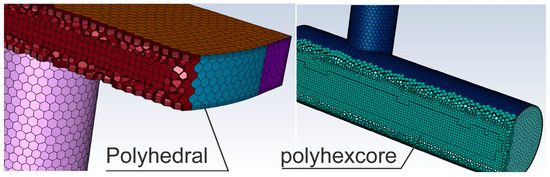
Figure 5.
Mesh structure of the flow domain.
During the investigation raised a hypothesis that the slot back wall with a guiding angle helps to achieve the required (narrowed) spray angle and, consequently, types of orifice shapes extended. The types of orifice shape for a semicircular atomizer in which the design search was carried out are shown in Figure 6.
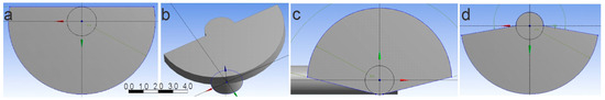
Figure 6.
Types of orifice shapes for a semicircular atomizer: (a) slot with flat angle, s = r; (b) slot with flat angle, s = 0; (c) tangent slot with obtuse angle, α = 152°; (d) slot with obtuse angle, s = 0, α = 150°.
2.3.2. Dividing the Output Surface into Several Equal Parts
Since the geometry of the outlet surface (slot orifice) is continuously long (Figure 7a) and semicylindrical, it is impossible to control the spray angle and perform optimization calculations to find the needed spray angle. Indeed, the assigning of calculation conditions or parameter limitations to obtain the required atomization angle over the whole strip outlet surface is impossible. Based on this, the outlet surface was divided into several equal parts—windows (w) by embedding the cutting planes formed with line extrusion using Boolean commands (Figure 7b).
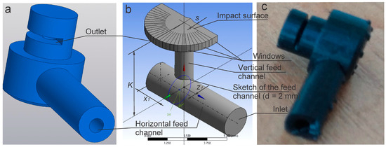
Figure 7.
Model of the nozzle (a), flow domain with the outlet surface divided into equal parts (b), and the printed nozzle (c).
The height of the extruded cutout must cover all values of h and rd and must also be arranged radially. The number of identified windows (w) were 30, and if taking into account the parameter s, there were 32 pcs. Dividing them into equal parts allows to select the number of windows that need to be covered with liquid during the calculations. For example, if up to 28 windows are assigned during optimization, there is a probability that the spraying angle will be reduced down to 160°–170° from 180°. It is supposed that the K, x1, and z1 parameters reduce the effects of turbulence; however, the range of their values is very limited.
2.3.3. Optimization of the Flat Sprayer Parameters
After the right inner shape of the nozzle clarified, the optimization calculations of the nozzle parameters with a semicircular impact surface were performed. Due to the influence of the turbulent flow formed in the vertical channel, the outlet flow uniformity critically decreased. A reason for turbulence was that the feed channel and the spray directions were mutually perpendicular to each other and had a short distance between them (K).
Calculations in Ansys Fluent® based on the theoretical studies and the parameters of nozzles with the reference option and value ratios, related equations that were introduced for the calculations and determined in advance. Optimization work can be performed during multiple stages depending on the result, and the parameters might be reconfigured in subsequent stages. The optimization conditions, input parameters, and parametric relations for optimization calculations of the nozzle parameters are given in Table A2. The target conditions (objectives) for optimization (an option) of the nozzle parameters are given in Table A3 and Table A4.
Table 1 presents the parameter limits used in optimization problems carried out for the definition of efficient structural parameters for the nozzle. The limit values are selected with regard to manufacturability.

Table 1.
Limits of the design parameters of the sprayer.
The optimization process is carried out using the direct optimization method. After the calculations, the candidate variants suggested by program are analyzed. If the variants do not meet the required spray quality, it is possible to recalculate with updating the parameters and manually searching for the right variants from the calculated row optimization table. Outlet velocity values as the calculation results determined from each assigned window (in our case, it is 28) can be evaluated by creating graphs in the Ansys platform or Excel® or Statistica® to evaluate the uniformity and angle of the spray. The indicators of the resultant variant evaluated visually and numerically are then compared with the indicators of the reference variant.
In general, the optimization calculations are conducted in two steps: first, for defining the more effective parameters of the nozzle, and then, to achieve to adequate uniformity of the spray.
2.4. Laboratory Experiments
2.4.1. Experimental Setup
After 3D modeling and optimization calculations, the nozzles were printed, and several experiments were carried out to check the workability. The experiments revealed the following spray quality characteristics: completeness and symmetricity of the spray, perpendicularity to the feed direction, uniformity, spray angle, fall angle, cross-spraying, and exit velocity indices. The determined fluid flow spray angles obtained during the simulations of the flow domain model were then compared with the experimental results (photos of the spray angle). To obtain the visual indices, video and photo recordings were made, and the spray parameters were then measured in programs such as KOMPAS 3D® and CorelDRAW® with high precision.
Figure 8 shows the scheme of the experimental setup with 10 output tubes. The experimental setup was developed using electronic devices designed for differential application technology of LMFs. In different experiments with modes of feed pressure, it is possible to use the required number of sprayers (1–10). The excess tubes are directed to the water tank. By blocking the outlet tubes one at a time, the feed rate was increased to 8–9 m/s; consequently, 9 feed modes can be selected. A ruler and an angle gauge are mounted on the measuring panel (14). The view positions of the video cameras (10) can also be changed to the top view position.
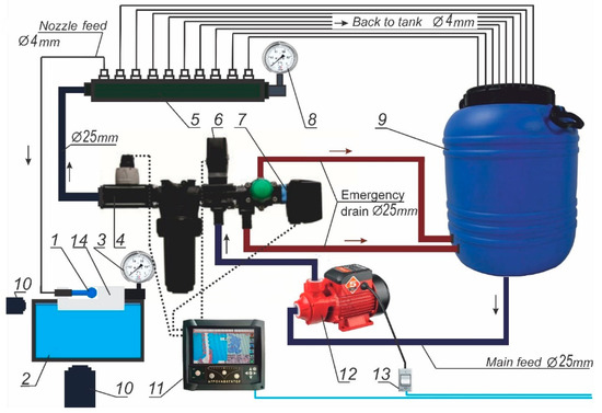
Figure 8.
Scheme of the experimental installation and tillage knife. 1—experimental nozzle; 2—water collection vessel (30 L); 3—tube pressure gauge (0.6 MPa); 4—flowmeter; 5—distributor; 6—electric main control valve; 7—electric proportional control valve; 8—distributor pressure gauge (0.6 MPa); 9—tank (50 L); 10—video cameras; 11—onboard computer; 12—surface pump (400 kW, 35 L/min) 13—switch; 14—measuring panel.
In the main experiments, water was used as the liquid medium. However, several experiments were conducted with fertilizer KAS-32 (UAN) to study the effect of liquid density and viscosity on the flow from the nozzle orifice and spray pattern. The temperature in the laboratory ranged from 20 to 28 °C. The density of KAS-32 was measured with the DMA 4500M, an electronic density measuring device, and showed 1312–1330 kg/m3.
2.4.2. Spray Uniformity Evaluation
The uniformity of the liquid mass flow at the outlet was evaluated using a handmade one-row multi-cell measuring vessel. The width of one cell in the measuring vessel was chosen relative to the width of the tillage knife, 15 mm, and the capacity was 10–15 mL (Figure 9). The measuring vessel should be held about 30–50 mm from the spray center to extract the liquid. Liquid should only be taken from the measuring vessel when there is a constant flow and a liquid spray is formed. After the sampling, the values of the liquid content in the measuring cells were measured, compared, then averaged, the maximum and minimum indicators determined. The average spray uniformity of the amount of liquid obtained in the vessel was determined as follows:
where Qo—average amount of liquid received in the cells of the vessel, mL.
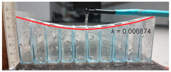
Figure 9.
Measuring vessel for the fluid spray uniformity.
Qmin and Qmax—the maximum and minimum amounts of liquid in the cells, mL.
Qc—the calculated amount of liquid in milliliters that can be filled in each cell during the required interval (5 s), and it is determined by the following formula:
where t—the time taken to obtain the required amount of fluid; in our case, it is 5 s.
Qs—quantity of liquid obtained in 1 s, mL. The last uniformity index is determined by dividing the definite value by a correction factor.
The uniformity indicators that are calculated using formula Equation (23) are then compared with the uniformity index (U) determined by computer modeling.
Because the atomization type is semiradial, to obtain the most correct uniformity evaluating indicators, it is effective if the overall sell mouth curve of the vessel would be circular. However, it is known that, in the short-term subsoil cavity, the spray shape does not form an exact semicircle. This can be monitored during the field experiments. Therefore, the magnitude of the line curvature depends on the cavity shape and dimensions.
The index of the curvature of the measuring vessel is defined (Figure 9). k is the uniformity correction factor.
where ks is the curvature indicator of the semicircle, and ka is the curvature indicator of the expected spray arc.
The radius of the semicircle will be equal to half the knife length.
2.4.3. The Spray Uniformity Evaluation by Wetting (Absorption) Shape and Dimensions
The recommended sprayers were tested under soil conditions to evaluate the uniformity and soil wetting quality. For this purpose, a trolley in the soil bin was equipped with tillage knives with mounted sprayers (Figure 10). The fluid supply and monitoring were performed using the experimental setup (Figure 8). The mounting depths of the knives were 6 and 9 cm. The working width of the knives was 150 mm. The speed of the trolley in the soil channel was very low (0.066 m/s). Two different sprayers were tested; the parameters of the first sprayer were h = 7 mm, Ds = 5 mm, d = 1.6 mm (d = d1), and s = R and the second with parameters of h = 5 mm, Ds = 5 mm, d1 = 1.2 mm (d > d1), and s = 0.1 mm.
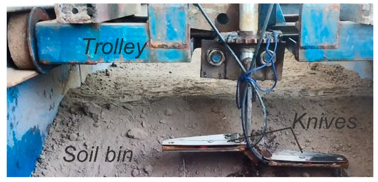
Figure 10.
The trolley equipped with knives and sprayers.
After passing the knife, the moistened strip of the soil was cleaned of dry soil particles and inspected. The height and width of the moistened strip were measured, and the uniformity was assessed [40]. This method is applicable for intra-soil spraying investigations.
3. Results and Discussions
3.1. The Sprayer Orifice Shape Search, and Results of the Optimization Calculations
The shape of the semiradial spraying orifice of the proposed flat fan sprayer should produce the optimal flow domain and required spray angle. Accordingly, the flow domain models with a flat angle, obtuse angle, and tangent shape were modeled in Ansys Fluent® and verified.
Figure 11 shows the 3D models of the investigated flow domains given by the velocity profile. In the sample with parameters s = 0, h = 3 mm, a deficit of fluid volume was observed due to low Atr in the orifice region (Figure 11a), and consequently, the fluid flow rate was significantly reduced. The Ai/Atr ratio was 2.666 at h = 0.3 mm and 1.14 at h = 0.7 mm. In the angled sample with parameters s = 0, h = 3 mm, α = 150°, it can be seen that most of the flow was streams along the two back walls with higher velocity (Figure 11b). This shortage was the main problem of the investigated designs (Figure 11c–f).
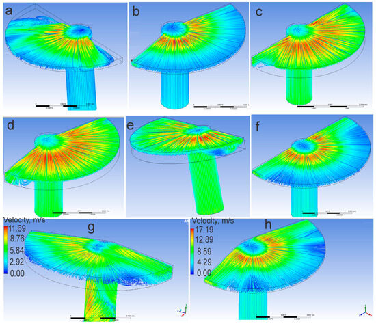
Figure 11.
Studied semicircular flow domain samples: s = 0, h = 3 mm (a); s = 0, h = 3 mm, α = 150° (b); s = 0, h = 7 mm (c); s = 0, h = 7 mm, α = 150° (d); d = 1.6 mm, h = 7 mm, s = 0.5 mm (e); d = 1.6 mm, h = 3 mm, s = 0.5 mm (f); tangential version, h = 7 mm, α = 152° (g); tangential version, h = 3 mm, α = 152° (h).
The optimization results show that the nozzle models with a flat angle are effective if an adequate value of h and s parameters is chosen. If s > 0.3 mm (in the range of h = 0.3–0.7 mm), it forms a spray with a flat angle. If h is higher than 0.5 mm, it again forms a spray with flat angles, and the flow is streams along the two back walls (even in the range of s = 0–0.3 mm), because the transition area increases. Nozzle variants with a flat guide angle eliminate the problem of flow accumulation in the two back walls observed above. The manufacturing process of nozzles with a flat angle is not complicated if compared to nozzles with an angled slot. According to the computational investigations, it was approved that the slot guide angle α1 (back wall angle) had no positive effect on forming the required spray angle.
In the parametric optimizations, the nozzle parameters with a suitable spray angle were obtained; however, the program tried to achieve an effective uniformity by decreasing the inlet velocity. Due to several extra calculations conducted, a positive effect for reduction of the turbulence was observed when d > d1 and at d = 2 mm.
In Figure 12, we visually compared the velocity profiles of three versions of nozzles (flow domain) calculated in ANSYS Fluent®. The first is a nozzle with the reference options, and the second and third versions are suggested by the program as effective variants (with right angle) of the nozzle, as it can be seen that, for the second and third options, the spray angle is reduced.
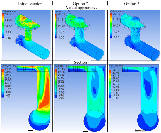
Figure 12.
Visual comparison of the effective and original options.
During the optimization calculations for spray uniformity and in the final selection, variants 31 and 28 showed higher spray uniformity (U) (Table 2). The inlet velocity is high, and the resultant indicators are within the effective parameters. In variant 28, the value of the s parameter is higher; consequently, the uniformity is lower.
Table 2.
Parameters and values of the selected variants in the optimization calculations for uniformity.
As can be seen, the overall spray uniformity is 74% for option 31 and 59% for option 28. Based on this, it can be considered that the spray is effective if the uniformity indicators obtained in the experimental results are above 60%. That is sufficient for applied studies and for intra-soil application operations. This can be explained by the fact that soil has a lumpy (or granular) structure during the first tillage passage, and the lumpiness fractions of the soil flowing over the tillage knife with a minimal height of 14 mm are different (smaller and larger than 14 mm), as seen in the field experiments. Lumps of different fractions randomly fall on the trace along the length of the knife, depending on their width and the unit speed, and as a consequence, the shape of the subsoil cavity is unstable. Accordingly, the uniformity index may decrease even it is high at the nozzle outlet.
Figure 13 shows the outlet velocities graphs of the selected candidate variants (points), with more effective uniformities obtained during the optimization calculations.
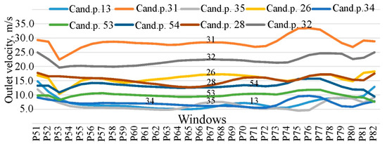
Figure 13.
The outlet velocity graphs obtained during the optimization calculations.
The determined optimal parameters are h = 5 mm, d = 2 mm, d1 is in the range of 0.5–0.8 mm, s is in the range of 0–0.2 mm, z1 is in the range of 0.1 ≥ z1 > R mm, and x1 is in the range of 1.4–2 mm. It is revealed that the d > d1 variants are more effective than the d = d1 variants. These uniform spray conditions (Figure 13) were obtained in the range of 4–9 m/s inlet velocity, where they provided several application dosages of LMFs.
By data processing using Ansys Fluent® and Statistica® and then comparing with graphical methods (KOMPAS-3D), the correct multiplication factor for Equation (11) was determined:
The deviation between the values determined by Equation (27) and the values determined graphically (KOMПAC-3D) in the identification method was 0–2%, and it is shown in Figure 14.
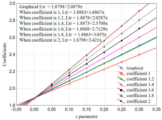
Figure 14.
Comparison of the Ltr determined with graphical methods (KOMPAS-3D) and Ltr determined by Equation (11) in different multiplying factors.
3.2. Results of the Experiments
3.2.1. Experimental Results for Checking the Parameters of the d > d1 Sprayer Type
During the laboratory experiments, the spray quality was evaluated, and the atomization shortcomings were determined. An excessive fall angle (γ) occurs when the h is very high (Figure 15a). The low spray uniformity (Figure 15b), the deviation in atomization symmetry (perpendicularity) (Figure 15c), and the deviation of the spray plane from the horizontal (Figure 15d) are observed under high turbulence conditions. The correct atomization with liquid film formation (Figure 15e) and correct atomization with a normal atomization plane and fall angle (Figure 15f) are observed for the right values of z1, x1, and s. For the correct atomization with a round-shaped liquid film, the liquid flows over the empty part of the nozzle impact surface and joins to the film (sheet) without breaking due to surface tension if the liquid velocity has an appropriate value. Under the influence of inertia, the round-shaped liquid film further disperses and scatters in the form of small droplets. The spray will be uniform if a regular liquid sheet of circular shape is formed around the semicircular slot (edge) during the atomization; the positive effect of the surface tension is noticeable in this situation.
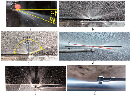
Figure 15.
Spraying behaviors: (a) excessive fall angle; (b) low spray uniformity; (c) atomization symmetry (perpendicularity) is broken; (d) atomization plane is deviated from the horizontal; (e) correct atomization with liquid film formation; (f) correct atomization with a normal atomization plane and fall angle (rear view).
Theoretically, when s = R and h ≥ R/2, the slot height does not adversely affect the flow velocity, as the slot area is equal to or greater than the feed channel area. The parameter s affects the atomization quality, as it narrows the vertical channel outlet and thus affects the atomization angle if s < R. Figure 16 shows the results of experiments conducted to study the influence of the parameter s on the quality of water atomization. When s = R, the transition area is maximized, and the spray increases up to 180°. When s = 0 and the h is very low, the transition area narrows, and the spray angle may decrease. According to the experiments, it was found that, at h = 0.5 mm, it is possible to obtain effective atomization angles only when s = 0 mm, s = 0.1 mm, and s = 0.2 mm. At s = 0.3 mm and above, the spray angle increases, or the atomization plane tilts relative to the horizontal.
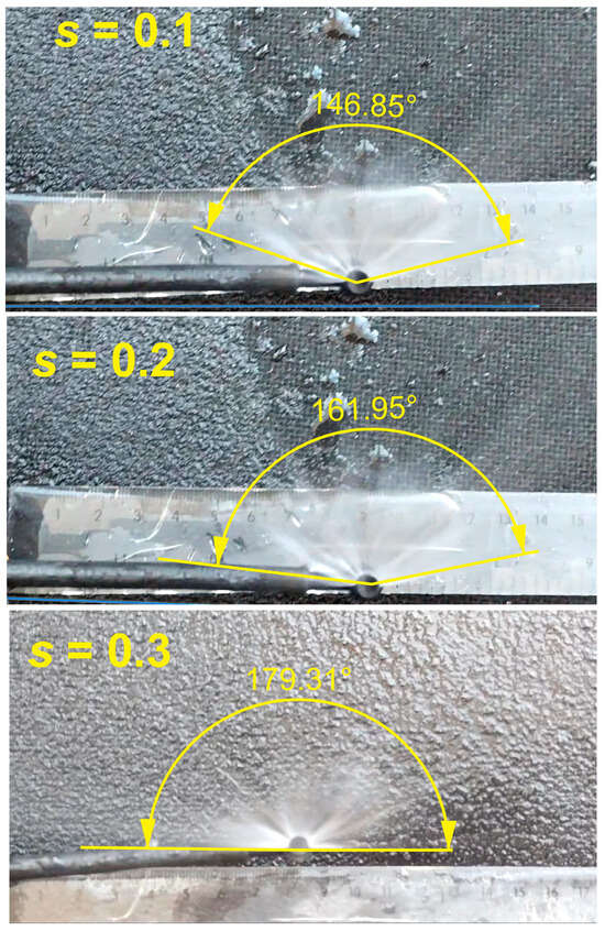
Figure 16.
Influence of parameter s on the atomization quality.
The applicability of the parametric optimized sprayers was tested by experiment, and the effect of the inlet velocity on the spray angle was determined. In Figure 17, the parameters of the investigated sprayers are h = 5 mm, Ds = 5 mm, d1 = 1.2 mm, and d = 2 mm.
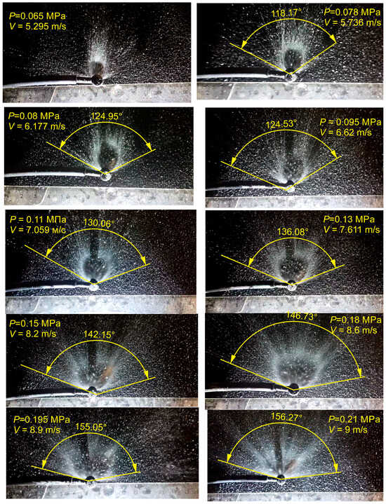
Figure 17.
Dependence of the spray angle on the inlet velocity (pressure).
As a result, the pressure indicators that form a permissible spraying angle were determined. When using 10 pieces of sprayer, the pressure that formed an acceptable spray angle was 0.11 MPa (and higher). The effective spray angle was formed at a pressure of 0.15 MPa (and above). In the system with 10 nozzles and when d1 = 1 mm, d1 = 1.2 mm, and d1 = 1.6 mm, the measured pressures were indicated as follows: P = 0.23–0.27 MPa, P = 0.18–0.195 MPa, and P = 0.14–0.16 MPa, consequently.
The mass flow rates in different pressure modes, atomization angles, and calculated flow thicknesses are presented in Table 3.
Table 3.
Determined atomization angles according to different delivery modes.
3.2.2. Absorption Form, Degree of Soil Moisture, and Spray Uniformity
The absorption form and soil moisture degree can show the spray quality and uniformity of the spray under the soil. The soil moisture indicators obtained using the nozzle with parameters d1 = 1.2 and s = 0.1 mm are the height of the moistened strip was 8–10 mm, and the width of the wetted strip was 7–9 cm. The reason for the low wetted strip width is the low atomization angle, because the s = 0.1 mm, with a low inlet diameter.
Figure 18 shows the soil wetting values of the sprayer with parameters h = 7 mm, Ds = 5 mm, d = 1.6 mm (d = d1), and s = R. The height of the wetted strip is 8–10 mm (Figure 18a), and the width is 13–14 cm (Figure 18b). The determined moisture content is 9–10%.
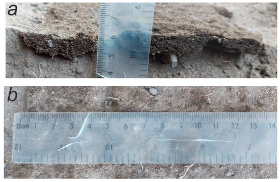
Figure 18.
Measuring of the soil moistening indicators of the sprayer with parameters h = 7 mm, Ds = 5 mm, d = 1.6 mm (d = d1), and s = R: (a) height; (b) width.
The spray uniformity can be seen from the moist layer shape or absorption form. If the shape of the wet layer is basically close to a rectangle and without any tearing, it means that the atomization process is uniform. If the equipment speed increases, the thickness of the moistened band thins because the spray starts to mix with soil particles, preserving their own aerosolized state and impact force. An effective intra-soil mixture of media (liquid and soil) occurs. No wetted layer with a thickness is formed at high equipment speeds.
Table 4 shows the results of the experiments to determine the atomization uniformity. The amount of liquid measured in each cell, their mean value, coefficient of variation, and corrected uniformity values according to the curvature index of the measuring vessel mouth line are presented in the table. Here, Uc are the corrected values of the uniformity indicators determined according to Equation (23), and the average indicator is 0.72. The value of the non-uniformity coefficient is about 10–30%. That is a low indicator if compared to other investigations ([15] (p. 12), [18] (p. 13)). However, for a nozzle with an asymmetric delivery channel and with a low value of K (Figure 1) and for intra-soil spraying conditions, the indicators are applicable. The curvature index of the defined semicircle is 0.013321, and k = 0.006874; accordingly, the correction factor is 1.08.
Table 4.
Measured spray uniformity values (h = 0.1 mm, d = 2 mm, d1 = 1.6, and s = 0.2 mm).
The experiments prove that the recommended sprayer parameters h = 0.5 mm, d = 2 mm, and Ds = 5 mm are applicable for use in the intra-soil application of LMFs and with uniformity qualities. They can be applied with variants in the range of d1 = 1–1.6 mm and s = 0–0.2 mm.
The CFD analysis and experiments showed that the negative effect of the inlet velocity on atomization uniformity is reduced when effective nozzle design parameters are established.
3.3. Field Experiments and Future Studies
According to the main goal of the study, the results of theoretical studies (Table A1), the spray angle dimensions obtained during CFD analyses and laboratory experiments (Figure 19) were compared. Importantly, these visual results were then compared with graphical determinations (Figure 19c) of the soil cavity parameters that formed during the trial of tillage knife movement at different velocities [33]. The comparisons allowed us to evaluate the applicability and practical use of the nozzles.
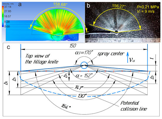
Figure 19.
Comparing the results: (a) CFD analyses; (b) laboratory experiments; (c) soil cavity parameters at different velocities of the tillage knife.
The practical use of the nozzle with the obtained effective angle and uniformity was also tested in production and field experiments (Figure A1). If the number of nozzles, the working width, and speed of the agricultural unit are known, it is possible to connect them with the delivery rate of LMFs.
The approximate fertilizer application dosage (q) can be determined by Equation (28) that is formulated from known equations.
where n is the number of nozzles in an agricultural unit, and M is the capacity of the loosener fertilizer, ha/h. It depends on the working width and speed of the agricultural unit. In real conditions, the work capacity agricultural unit depends on many factors. A—feed channel area. It depends on the feed channel diameter and parameter s.
The determined approximate fertilizer application dosage (q) dependent on the inlet velocity and parameter s, as well as the unit speed, is shown in Table A5 and Table A6. These data can also be determined for nozzles with other feed channel diameters. When the feed diameter d1 = 1–1.6 mm, an agricultural unit speed of 5–12 km/h, and a fluid inlet velocity of 5–9 m/s, the nozzles provide a delivery dosage of 100–400 L/ha.
By increasing the number of sprayers mounted on the tillage knife, it is possible to move to the differentiated introduction approach of the LMFs. Experiments have shown that the nozzles are suitable for applying KAS-32 even with a minimum feed diameter of 1 mm.
During the research, atomization uniformity of up to 74% was achieved; however, further fundamental research is required to obtain higher uniformity (85–90%). The influence of fluid viscosity and the effect of parameters z1 and x1 on the atomization uniformity, as well as the impact force of the outlet flow and mixing processes, are the objectives of future research.
4. Conclusions
A spray nozzle 3D model of the universal deep loosener fertilizer for the intra-soil application of LMFs was developed and optimized using Ansys Fluent®, then tested in laboratory and field experiments. The optimization calculations performed with the 3D model of the liquid flow domain that streams through the nozzle obtained the optimal nozzle parameters and their limits.
We experimentally revealed that the d > d1 variants were more effective than the d = d1 variants.
The modeled spray guide (back wall) angle α1 had no positive effect on obtaining the needed spray angle or on the spray uniformity. The spray rate and spray angle can be adjusted due to parameter s. It was found that, when the spray angle was within s = 0–0.2 mm, it formed a spray angle range of 140°–175°.
Spray uniformity up to 74% was achieved for nozzles with bi-level and mutual perpendicular inlet and outlet flow directions.
The suggested value of Ds was 5–8 mm. The effective value was 5 mm, and as the radius increased, the fall angle was adversely affected. To obtain a horizontal spray (flow), the impact surface should be horizontal.
The formula for determining the transition window arc length (Ltr) and the effective coefficient was introduced. The deviation between the values determined by the formula and the values determined in the graphical visualization method was 0–2%.
Experiments and CFD analyses showed that, when effective design parameters of the sprayer are established, the inlet velocity does not adversely affect the atomization uniformity.
The proposed nozzles were suitable for the application of LMFs with a density of 1300–1330 kg/m3, and accordingly, it can be concluded that the designed nozzle is applicable for the intra-soil application of liquid mineral fertilizers.
Author Contributions
Conceptualization, S.N. and K.T.; methodology, K.T.; software, K.T. and A.S.; validation, N.K., A.M. and M.R.; formal analysis, A.M.; investigation, K.T.; resources, K.T.; data curation, N.K. and M.R.; writing—original draft preparation, K.T.; writing—review and editing, A.S. and K.T.; visualization, K.T. and A.S.; supervision, S.N.; project administration, S.N.; funding acquisition, S.N. All authors have read and agreed to the published version of the manuscript.
Funding
This research was funded by the Science Committee of the Ministry of Science and Higher Education of the Republic of Kazakhstan, Grant No. AP19674514.
Data Availability Statement
The data are contained in the article.
Acknowledgments
We are grateful to Tahsin Engin, Professor at Istanbul Technical University, for his advice on CFD calculations.
Conflicts of Interest
The authors declare no conflicts of interest.
Appendix A
Table A1.
Dependence of the spray angle on the parameters s, R.
Table A1.
Dependence of the spray angle on the parameters s, R.
| s | d1/2 | L4 | Ltr (Graphical) | Ltr with Equation (27) | Ltr with Equation (11) | Lo | The Angle Limits |
|---|---|---|---|---|---|---|---|
| 0.4 | |||||||
| 0.5 | 1.007 | 2.498092 | 2.44633808 | 2.412256 | 7.286101667 | 145–167 | |
| 0.6 | 1.212 | 2.760629 | 2.730054005 | 2.7033 | 8.051834583 | flat angle | |
| 0.7 | 1.419 | 3.050659 | 3.029897048 | 2.99806 | 8.897755417 | flat angle | |
| 0.8 | 1.629 | 3.351032 | 3.335850878 | 3.296536 | 9.773843333 | flat angle | |
| 0.9 | 1.841 | 3.656431 | 3.644785371 | 3.598728 | 10.66459042 | flat angle | |
| 0.3 | |||||||
| 0.5 | 1.007 | 2.214297 | 2.196760752 | 2.166754 | 6.45836625 | 126–148 | |
| 0.6 | 1.212 | 2.513274 | 2.501888159 | 2.463234 | 7.3303825 | 147–168 | |
| 0.7 | 1.419 | 2.81919 | 2.81113048 | 2.76343 | 8.2226375 | flat angle | |
| 0.8 | 1.629 | 3.128309 | 3.122278315 | 3.067342 | 9.124234583 | flat angle | |
| 0.9 | 1.841 | 3.43914 | 3.434447087 | 3.37497 | 10.030825 | flat angle | |
| 0.2 | |||||||
| 0.5 | 1.007 | 1.982313 | 1.977691757 | 1.934244 | 5.78174625 | 113–132 | |
| 0.6 | 1.212 | 2.29276 | 2.289631391 | 2.23616 | 6.687216667 | 135–153 | |
| 0.7 | 1.419 | 2.604767 | 2.602502722 | 2.541792 | 7.597237083 | 161–174 | |
| 0.8 | 1.629 | 2.917563 | 2.915845112 | 2.85114 | 8.50955875 | flat angle | |
| 0.9 | 1.841 | 3.230801 | 3.229452658 | 3.164204 | 9.423169583 | flat angle | |
| 0.1 | |||||||
| 0.5 | 1.007 | 1.772154 | 1.771610666 | 1.714726 | 5.1687825 | 100–118 | |
| 0.6 | 1.212 | 2.085893 | 2.085518012 | 2.022078 | 6.083854583 | 122–139 | |
| 0.7 | 1.419 | 2.399801 | 2.085518012 | 2.333146 | 6.999419583 | 147–160 | |
| 0.8 | 1.629 | 2.713799 | 2.713588779 | 2.64793 | 7.915247083 | 173–180 | |
| 0.9 | 1.841 | 3.027847 | 3.027681645 | 2.96643 | 8.831220417 | flat angle | |
| 0 | |||||||
| 0.5 | 1.007 | 1.570796 | 1.570796327 | 1.5082 | 4.581488333 | 88–105 | |
| 0.6 | 1.212 | 1.884956 | 1.884955592 | 1.820988 | 5.497788333 | 110–126 | |
| 0.7 | 1.419 | 2.199115 | 2.199115 | 2.137492 | 6.414085417 | 134–147 | |
| 0.8 | 1.629 | 2.513274 | 2.513274 | 2.457712 | 7.3303825 | 162–168 | |
| 0.9 | 1.841 | 2.827433 | 2.827433388 | 2.781648 | 8.246679583 | flat angle |
The deviation between the graphical Ltr and Ltr obtained by Equation (27) is 0–2%.
Table A2.
Input parameters and parametric relations for the optimization calculations of the nozzle parameters.
Table A2.
Input parameters and parametric relations for the optimization calculations of the nozzle parameters.
| ID | Parameter Name | Symbols | Value | Unit |
|---|---|---|---|---|
| 1 | 2 | 3 | 4 | 5 |
| Input Parameters | ||||
| Geometry (A1) | ||||
| P1 | Extrude2.FD1 | K | 5 | mm |
| P2 | Extrude4.FD1 | H | 0.7 | mm |
| P3 | ZXPlane.R5 | R (d1) | 1 | mm |
| P74 | Plane4.R16 | rd (Ds/2) | 4 | mm |
| P148 | XYPlane.R2 | d/2 | 1 | mm |
| Fluent (with Fluent Meshing) (B1) | ||||
| P154 | velocity | Vi | 6000 | mm s−1 |
| Output Parameters | ||||
| Fluent (with Fluent Meshing) (B1) | Value | Unit | ||
| P156 | out-vfr-7-op | Q7 | −779.19213 | mm3 s−1 |
| P157 | out-vfr-8-op | Q8 | −746.50933 | mm3 s−1 |
| P158 | out-vfr-10-op | Q10 | −747.07094 | mm3 s−1 |
| P159 | out-vfr-12-op | Q712 | −687.25524 | mm3 s−1 |
| P160 | out-vfr-21-op | Q21 | −623.98351 | mm3 s−1 |
| P161 | out-vfr-24-op | Q24 | −659.62593 | mm3 s−1 |
| P162 | out-vfr-25-op | Q25 | −729.6332 | mm3 s−1 |
| P163 | out-vfr-26-op | Q26 | −601.17009 | mm3 s−1 |
| P164 | out-vfr-28-op | Q28 | −156.66363 | mm3 s−1 |
| P165 | out-vfr-29-op | Q29 | −273.94256 | mm3 s−1 |
| P166 | out-vfr-30-op | Q30 | −1392.3157 | mm3 s−1 |
| P169 | out-vfr-1-op | Q1 | −416.8453 | mm3 s−1 |
| P170 | out-vfr-2-op | Q2 | −219.89692 | mm3 s−1 |
| P171 | out-vfr-3-op | Q3 | −443.29693 | mm3 s−1 |
| P172 | out-vfr-4-op | Q4 | −665.22239 | mm3 s−1 |
| P173 | out-vfr-5-op | Q5 | −789.99409 | mm3 s−1 |
| P174 | out-vfr-6-op | Q6 | −816.03901 | mm3 s−1 |
| P175 | out-vfr-9-op | Q9 | −747.40171 | mm3 s−1 |
| P176 | out-vfr-11-op | Q11 | −719.43089 | mm3 s−1 |
| P177 | out-vfr-13-op | Q13 | −681.33977 | mm3 s−1 |
| P178 | out-vfr-14-op | Q14 | −668.4121 | mm3 s−1 |
| P179 | out-vfr-15-op | Q15 | −646.98662 | mm3 s−1 |
| P180 | out-vfr-16-op | Q16 | −626.79214 | mm3 s−1 |
| P181 | out-vfr-17-op | Q17 | −625.36054 | mm3 s−1 |
| P182 | out-vfr-18-op | Q18 | −628.43384 | mm3 s−1 |
| P183 | out-vfr-19-op | Q19 | −626.88525 | mm3 s−1 |
| P184 | out-vfr-20-op | Q20 | −627.1045 | mm3 s−1 |
| P185 | out-vfr-22-op | Q22 | −605.09348 | mm3 s−1 |
| P186 | out-vfr-23-op | Q23 | −607.52501 | mm3 s−1 |
| P187 | out-vfr-27-op | Q27 | −314.46172 | mm3 s−1 |
| P196 | back-flux1-op | P | 0 | MPa |
| P197 | back-flux2-op | P | −0.009623637 | MPa |
| P228 | inlet-area-op | Ai | 3.128594 | mm2 |
| P230 | inl-vfr-op | Qi | 18771.563 | mm3 s−1 |
| P231 | inl-vfr-/28-constant-op | Qwcons | 670.41299 | mm3 s−1 |
| P232 | sum-28-vfr-op | −17064.724 | mm3 s−1 | |
| . w = 28 | ||||
| P233 | inl-/-28-ratio-vfr-op | −1.1000215 | ||
| P262 | out-full-veloc-ave-op | Voavg | 3935.0078 | mm s−1 |
| P263 | out-vfr-full-op | Qo | −18873.885 | mm3 s−1 |
| P264 | area-wei-ave-veloc-out-op | VAwaV | 3667.1295 | mm s−1 |
| P265 | sd-sum-28-op | −609.45439 | mm3 s−1 | |
| P267 | max-velo-out-op | Vomax | 10559.475 | mm s−1 |
| P268 | cons-ratio-op | −0.90907305 | ||
| P269 | cret-1-op (S28) | 1.2100474 | ||
| P150 | Output Area | Ao | 8.79645943 | mm2 |
| P151 | trans Area | Atr | 2.199114858 | mm2 |
| P152 | Inl Out ratio | Ao/Ai | 2.811633414 | |
| P153 | Trans Inl ratio | Atr/Ai | 0.898689128 | |
| P155 | Sel 30 Area | Aw | 0.293215314 | mm2 |
| P198 | Ratio1 | Q1/Qwcons | −0.621773901 | |
| P199 | Ratio 2 | Q2/Qwcons | −0.328002177 | |
| P200 | Ratio 3 | Q3/Qwcons | −0.661229625 | |
| P201 | Ratio 4 | Q4/Qwcons | −0.992257608 | |
| P202 | Ratio 5 | Q5/Qwcons | −1.178369306 | |
| P203 | Ratio 6 | Q6/Qwcons | −1.217218375 | |
| P204 | Ratio 7 | Q7/Qwcons | −1.16225691 | |
| P205 | Ratio 8 | Q8/Qwcons | −1.113506661 | |
| P206 | Ratio 9 | Q9/Qwcons | −1.114837751 | |
| P207 | Ratio 10 | Q10/Qwcons | −1.114344369 | |
| P208 | Ratio 11 | Q11/Qwcons | −1.073115976 | |
| P209 | Ratio 12 | Q12/Qwcons | −1.025122201 | |
| P210 | Ratio 13 | Q13/Qwcons | −1.01629858 | |
| P211 | Ratio 14 | Q14/Qwcons | −0.997015437 | |
| P212 | Ratio 15 | Q15/Qwcons | −0.965056808 | |
| P213 | Ration16 | Q16/Qwcons | −0.93493436 | |
| P214 | Ratio 17 | Q17/Qwcons | −0.93279896 | |
| P215 | Ratio 18 | Q18/Qwcons | −0.937383149 | |
| P216 | Ratio 19 | Q19/Qwcons | −0.935073245 | |
| P217 | Ratio 20 | Q20/Qwcons | −0.935400282 | |
| P218 | Ratio 21 | Q21/Qwcons | −0.930744958 | |
| P219 | Ratio 22 | Q22/Qwcons | −0.902568251 | |
| P220 | Ratio 23 | Q23/Qwcons | −0.906195165 | |
| P221 | Ratio 24 | Q24/Qwcons | −0.983909828 | |
| P222 | Ratio 25 | Q25/Qwcons | −1.088333924 | |
| P223 | Ratio 26 | Q26/Qwcons | −0.896716053 | |
| P224 | Ratio 27 | Q27/Qwcons | −0.469056723 | |
| P225 | Ratio 28 | Q28/Qwcons | −0.233682271 | |
| P226 | Ratio 29 | Q29/Qwcons | −0.408617619 | |
| P227 | Ratio 30 | Q30/Qwcons | −2.076802987 | |
| P234 | w2 | −219.89692 | mm3 s−1 | |
| P235 | w3 | −443.29693 | mm3 s−1 | |
| P236 | w4 | −665.22239 | mm3 s−1 | |
| P237 | w5 | −789.99409 | mm3 s−1 | |
| P238 | w6 | −816.03901 | mm3 s−1 | |
| P239 | w7 | −779.19213 | mm3 s−1 | |
| P240 | w8 | −746.50933 | mm3 s−1 | |
| P241 | w9 | −747.40171 | mm3 s−1 | |
| P242 | w10 | −747.07094 | mm3 s−1 | |
| P243 | w11 | −719.43089 | mm3 s−1 | |
| P244 | w12 | −687.25524 | mm3 s−1 | |
| P245 | w13 | −816.03901 | mm3 s−1 | |
| P246 | w14 | −668.4121 | mm3 s−1 | |
| P247 | w15 | −646.98662 | mm3 s−1 | |
| P248 | w16 | −626.79214 | mm3 s−1 | |
| P249 | w17 | −625.36054 | mm3 s−1 | |
| P250 | w18 | −628.43384 | mm3 s−1 | |
| P251 | w19 | −626.88525 | mm3 s−1 | |
| P252 | w20 | −627.1045 | mm3 s−1 | |
| P253 | w21 | −623.98351 | mm3 s−1 | |
| P254 | w22 | −605.09348 | mm3 s−1 | |
| P255 | w23 | −607.52501 | mm3 s−1 | |
| P256 | w24 | −659.62593 | mm3 s−1 | |
| P257 | w25 | −729.6332 | mm3 s−1 | |
| P258 | w26 | −601.17009 | mm3 s−1 | |
| P259 | w27 | −314.46172 | mm3 s−1 | |
| P260 | w28 | −156.66363 | mm3 s−1 | |
| P261 | w29 | −273.94256 | mm3 s−1 | |
Where P156–P187—volume flow rate (flow rate) from each outlet window. P230—volume flow rate (flow rate) of the entered liquid. P231—the volume flow rate (flow rate) for one outlet window (a constant value for the 28 outlet windows). P232—the sum of the outlet volume of liquid from 28 output windows. P233—the ratio of P230 to P232; that is, the ratio of the inlet volume flow rate and the outlet volume flow rate from the 28 windows. It should be minimized (maximized) to −1. P265—the average value of the flow volume from the 28 outlet windows. P268—the relationship between P231 and P265. It should be close to −1. P269—the critical ratio for the 28 window output values, i.e., the ratio between P268 and P233 (S28). It should be close to −1. From Ratio1 to Ratio30—the ratio between volume flow rate (flow rate) from each window and P231.
Table A3.
Target conditions (objectives) for the optimization (an option) of the nozzle parameters.
Table A3.
Target conditions (objectives) for the optimization (an option) of the nozzle parameters.
| Name and Parameters | Objective | |
|---|---|---|
| P233—inl-/-28-ratio-vfr-op | Minimize | −1 |
| P268—cons-ratio-op | Minimize | −1 |
| P269—cret-1-op | Minimize | 1 |
| P199—Ratio 2 | Minimize | −1 |
| P226—Ratio 29 | Minimize | −1 |
| P198—Ratio1 | Minimize | −1 |
| P227—Ratio 30 | Minimize | −1 |
| P169—out-vfr-1-op | Minimize | −1 |
| P166—out-vfr-30-op | Minimize | −1 |
Table A4.
Target conditions (objectives) for the optimization of the nozzle parameters for the objective of spray uniformity.
Table A4.
Target conditions (objectives) for the optimization of the nozzle parameters for the objective of spray uniformity.
| Name | Parameter | Objective | ||
|---|---|---|---|---|
| Type | Target | Tolerance | ||
| Minimize P97 | P97—Ratio const | Minimize | −1 | |
| Minimize P94 | P94—Ratio out inlet | Minimize | −1 | |
| Minimize P17 | P17—vfr-00-op | Minimize | 0 | |
| Minimize P18 | P18—vfr-01-op | Minimize | 0 | |
| Minimize P48 | P48—vfr-31-op | Minimize | 0 | |
| Minimize P47 | P47—vfr-30-op | Minimize | 0 | |
| Minimize P51 | P51—max-vel-00-op | Minimize | 0 | |
| Minimize P52 | P52—max-vel-01-op | Minimize | 0 | |
| Minimize P81 | P81—max-vel-30-op | Minimize | 0 | |
| Minimize P82 | P82—max-vel-31-op | Minimize | 0 | |
| Seek P110 = 1 | P110—eq2-op | Seek Target | 1 | 0.001 |
| Seek P111 = 1 | P111—eq1-op | Seek Target | 1 | 0.001 |
| Seek P112 = 1 | P112—End ratio | Seek Target | 1 | 0.001 |
Appendix B

Figure A1.
The working organ (a) of the universal deep loosener fertilizer with tillage knives, and a flat fan spraying nozzle (b).
Figure A1.
The working organ (a) of the universal deep loosener fertilizer with tillage knives, and a flat fan spraying nozzle (b).

Table A5.
Approximate dosage of liquid mineral fertilizers in relation to parameter s of a nozzle with d1 = 1.2 mm (L/ha).
Table A5.
Approximate dosage of liquid mineral fertilizers in relation to parameter s of a nozzle with d1 = 1.2 mm (L/ha).
| s | mm | 0 | 0.1 | 0.2 | ||||||||||||
| Vi | m/s | 5 | 6 | 7 | 8 | 9 | 5 | 6 | 7 | 8 | 9 | 5 | 6 | 7 | 8 | 9 |
| Va, km/h | 12 | 73 | 88 | 102 | 117 | 131 | 81 | 97 | 113 | 129 | 145 | 89 | 107 | 124 | 142 | 160 |
| 11 | 80 | 96 | 112 | 127 | 143 | 88 | 106 | 123 | 141 | 158 | 97 | 116 | 136 | 155 | 174 | |
| 10 | 88 | 105 | 123 | 140 | 158 | 97 | 116 | 137 | 155 | 174 | 107 | 128 | 149 | 170 | 192 | |
| 9 | 97 | 117 | 136 | 156 | 175 | 108 | 129 | 151 | 172 | 194 | 118 | 142 | 166 | 189 | 213 | |
| 8 | 110 | 131 | 153 | 175 | 197 | 121 | 145 | 169 | 194 | 218 | 133 | 160 | 186 | 213 | 239 | |
| 7 | 125 | 150 | 175 | 200 | 225 | 138 | 166 | 194 | 221 | 249 | 152 | 182 | 213 | 243 | 273 | |
| 6 | 146 | 175 | 204 | 233 | 262 | 161 | 194 | 226 | 258 | 290 | 177 | 213 | 248 | 283 | 319 | |
| 5 | 175 | 210 | 245 | 280 | 315 | 194 | 232 | 271 | 309 | 348 | 213 | 255 | 298 | 340 | 383 | |
Table A6.
Approximate dosage of liquid mineral fertilizers in relation to parameter s of a nozzle with d1 = 1.4 mm (L/ha).
Table A6.
Approximate dosage of liquid mineral fertilizers in relation to parameter s of a nozzle with d1 = 1.4 mm (L/ha).
| s | mm | 0 | 0.1 | 0.2 | ||||||||||||
| Vi | m/s | 5 | 6 | 7 | 8 | 9 | 5 | 6 | 7 | 8 | 9 | 5 | 6 | 7 | 8 | 9 |
| Va, km/h | 12 | 85 | 102 | 119 | 136 | 153 | 93 | 112 | 130 | 149 | 167 | 101 | 121 | 141 | 161 | 181 |
| 11 | 93 | 112 | 130 | 149 | 167 | 101 | 122 | 142 | 162 | 182 | 110 | 132 | 154 | 176 | 198 | |
| 10 | 102 | 123 | 143 | 163 | 184 | 112 | 134 | 156 | 178 | 200 | 121 | 145 | 169 | 193 | 218 | |
| 9 | 114 | 136 | 159 | 181 | 204 | 124 | 149 | 173 | 198 | 223 | 134 | 161 | 188 | 215 | 242 | |
| 8 | 128 | 153 | 179 | 204 | 230 | 139 | 167 | 195 | 223 | 250 | 151 | 181 | 211 | 242 | 272 | |
| 7 | 146 | 175 | 204 | 233 | 262 | 159 | 191 | 223 | 254 | 286 | 173 | 207 | 242 | 276 | 311 | |
| 6 | 170 | 204 | 238 | 272 | 306 | 186 | 223 | 260 | 297 | 334 | 201 | 242 | 282 | 322 | 362 | |
| 5 | 204 | 245 | 286 | 326 | 367 | 223 | 267 | 312 | 356 | 400 | 242 | 290 | 338 | 386 | 435 | |
References
- Filcheva, E.; Ilieva, R.; Lubenova, I.; Hristov, B.; Hristova, M. Humus state of Bulgarian chernozems. Modern State of Chernozems. Proc. II Int. Sci. Conf. 2018, 1, 69–76. [Google Scholar]
- Ghazaryan, H.G.; Kroyan, S.; Manukyan, N.; Kalashian, M.Y. Current state of humus in irrigated meadow-brown soils in the Republic of Armenia. Ann. Agrar. Sci. 2016, 14, 307–310. [Google Scholar] [CrossRef]
- Tibbett, M.; Gil-Martínez, M.; Fraser, T.D.; Green, I.D.; Duddigan, S.; De Oliveira, V.H.; Raulund-Rasmussen, K.; Sizmur, T.; Díaz, A. Long-term acidification of pH neutral grasslands affects soil biodiversity, fertility and function in a heathland restoration. Catena 2019, 180, 401–415. [Google Scholar] [CrossRef]
- Nguemezi, C.; Tixier, P.; Yemefack, M.; Tsozué, D.; Silatsa, T. Soil quality and soil fertility status in major soil groups at the Tombel area, South-West Cameroon. Heliyon 2020, 6, e03432. [Google Scholar] [CrossRef] [PubMed]
- Nukeshev, S.; Eskhozhin, D.; Mamyrbayeva, I.; Karaivanov, D.; Gubasheva, A.; Tleumbetov, K.; Kossatbekova, D.; Tanbayev, K. Mathematical Modelling and Designing of a Universal Conical Spreader for Granular Material. Acta Technol. Agric. 2023, 26, 152–158. [Google Scholar] [CrossRef]
- Nukeshev, S.O.; Yeskhozhin, K.D.; Kusainov, R.K. Substantiation of the constructive and technological scheme of the machine for intra soil differentiated three-layer introduction of mineral fertilizers. Int. Sci. J. Mech. Agric. 2016, 3, 3–6. [Google Scholar]
- Altintas, S.; Funda Eryilmaz, A. The effects of mineral and liquid organic fertilizers on some nutritional characteristics of bell pepper. Afr. J. Biotechnol. 2012, 11, 6470–6475. [Google Scholar] [CrossRef]
- Assefa, B.; Chen, Y.; Buckley, K.; Akinremi, W. Effects of manure injection tool type and tool spacing on soil nutrient levels and spring barley performance. Can. Biosyst. Eng./Le Génie Des Biosystèmes Au Can. 2006, 48, 2.45–2.54. [Google Scholar]
- Yuvraj, G.K.; Thakare, S.K.; Deshmukh, M.M. Liquid fertilizer application system on planting mechanism a concept. Natl. Acad. Agric. Sci. 2015, 33, 3789–3791. [Google Scholar]
- Yadav, M.R.; Kumar, R.; Parihar, C.M.; Yadav, R.K.; Jat, S.L.; Ram, H.; Meena, R.K.; Singh, M.B.; Verma, A.P.; Ghoshand, A.; et al. Strategies for improving nitrogen use efficiency: A review. Agric. Rev. 2017, 38, 29–40. [Google Scholar] [CrossRef]
- Cândido de Souza, Á.H.; Lorenzoni, M.Z.; Rezende, R.; Santos, F.A.S.; Seron, C.D.C.; Andrean, A.F.B.A. Fertigation and foliar application with liquid mineral fertilizer doses on lettuce. Sci. Agrar. 2018, 19, 37–43. [Google Scholar]
- Chaorakam, I.; Sukcharoen, A.; Jaiphong, T. Field Evaluation of Subsoiling and Liquid Fertilizer Injection for Minimum Tillage of Sugarcane Planter (Part 1)—Effects of Subsoiling and Liquid Fertilizer Injection on Germination Test. Int. J. Appl. Sci. Technol. 2012, 2, 234–242. [Google Scholar]
- Munroe, J. Soil Fertility Handbook: Vol. Publication 611, 3rd ed.; Ontario Ministry of Agriculture, Food and Rural Affairs (OMAFRA), Ed.; Queen’s Printer for Ontario: Toronto, ON, Canada, 2018. Available online: http://www.omafra.gov.on.ca/english/crops/pub611/pub611.pdf (accessed on 23 November 2021).
- Cieniawska, B.; Parafiniuk, S.; Kluza, P.A.; Otachel, Z. Matching the Liquid Atomization Model to Experimental Data Obtained from Selected Nozzles. Appl. Sci. 2023, 13, 4433. [Google Scholar] [CrossRef]
- Wawrzosek, J.; Parafiniuk, S. The Use of the Permutation Algorithm for Suboptimising the Position of Used Nozzles on the Field Sprayer Boom. Appl. Sci. 2022, 12, 4359. [Google Scholar] [CrossRef]
- Alheidary, M.H.R. Influence of nozzle type, working pressure, and their interaction on droplets quality using knapsack sprayer. Iraqi J. Agric. Sci. 2019, 50, 857–866. [Google Scholar] [CrossRef][Green Version]
- Makhnenko, I.; Alonzi, E.R.; Fredericks, S.A.; Colby, C.M.; Dutcher, C.S. A review of liquid sheet breakup: Perspectives from agricultural sprays. J. Aerosol Sci. 2021, 157, 105805. [Google Scholar] [CrossRef]
- Kluza, P.A.; Kuna-Broniowska, I.; Parafiniuk, S. Modeling and Prediction of the Uniformity of Spray Liquid Coverage from Flat Fan Spray Nozzles. Sustainability 2019, 11, 6716. [Google Scholar] [CrossRef]
- Nukeshev, S.; Yeskhozhin, K.; Karaivanov, D.; Ramaniuk, M.; Akhmetov, E.; Saktaganov, B.; Tanbayev, K. A Chisel Fertilizer for In-Soil Tree-Layer Differential Application in Precision Farming. Int. J. Technol. 2023, 14, 109–118. [Google Scholar] [CrossRef]
- Chen, Y. A Liquid Manure Injection Tool Adapted to Different Soil Conditions. Trans. ASAE 2002, 45, 1729–1736. [Google Scholar] [CrossRef]
- Tanbayev, K.; Nukeshev, S.; Sugirbay, A. Performance Evaluation of Tillage Knife Discharge Microchannel. Acta Technol. Agric. 2022, 25, 169–175. [Google Scholar] [CrossRef]
- Tanbayev, K.; Nukeshev, S.; Tahsin, E.; Saktaganov, B. Flat Spray Nozzle for Intra-Soil Application of Liquid Mineral Fertilizers. Acta Technol. Agric. 2023, 26, 65–71. [Google Scholar] [CrossRef]
- Majumdar, N.; Tirumkudulu, M.S. Dynamics of radially expanding liquid sheets. Phys. Rev. Lett. 2018, 120, 164501. [Google Scholar] [CrossRef]
- Lightfoot, M. Fundamental classification of atomization processes. At. Sprays 2009, 19, 1065–1104. [Google Scholar] [CrossRef]
- Watson, E.J. The radial spread of a liquid jet over a horizontal plane. J. Fluid Mech. 1964, 20, 481–499. [Google Scholar] [CrossRef]
- Wu, D.; Guillemin, D.; Marshall, A.W. A modeling basis for predicting the initial sprinkler spray. Fire Saf. J. 2007, 42, 283–294. [Google Scholar] [CrossRef]
- Clanet, C.; Villermaux, E. Life of a smooth liquid sheet. J. Fluid Mech. 2002, 462, 307–340. [Google Scholar] [CrossRef]
- Pazhi, D.G.; Galustov, V.S. Fundamentals of the Liquid Atomization Techniques; Chimiya: Moscow, Russia, 1984. (In Russian) [Google Scholar]
- Lechler GmbH. Lechler Agricultural Technology Nozzles. 2017. Available online: https://www.lechler.com/de-en/products-nozzles-spray-technology-systems/product-range/agriculture (accessed on 10 October 2023).
- Fan Nozzle. BETE Spray Nozzles. 2023. BETE Spray Technology. Available online: https://bete.com/pattern/fan-spray-pattern (accessed on 10 October 2023).
- Azuma, T.; Hoshino, T. The radial flow of a thin liquid film: 2nd report, liquid film thickness. Bull. JSME 1984, 27, 2747–2754. [Google Scholar] [CrossRef]
- Azuma, T.; Hoshino, T. The radial flow of a thin liquid film: 3rd report, velocity profile. Bull. JSME 1984, 27, 2755–2762. [Google Scholar] [CrossRef]
- Tanbayev, K.; Nukeshev, S.O.; Tahsin, E. Determination the cavity shape and sizes on the trail of the tillage knife for liquid fertilizer application. Sci. J. Bull. Sci. S. Seifullin Kazakh Agro Tech. Res. Univ. 2023, 2, 99–108. (In Kazakh) [Google Scholar]
- Zaree, M.; Parashkoohi, M.G.; Ghafori, H.; Zamani, D.M. Investigation of flow pattern in an innovative nozzle: An experimental 655 and numerical study in agricultural systems. J. Saudi Soc. Agric. Sci. 2023. [Google Scholar] [CrossRef]
- Becze, S.; Vuşcan, G.I. Comparison study between two types of nozzles for a turbocharger balancing machine using ANSYS software. MATEC Web Conf. 2019, 299, 04007. [Google Scholar] [CrossRef]
- Wang, J.; Liang, Q.; Zeng, T.; Zhang, X.; Wei, F.; Lan, Y. Drift Potential Characteristics of a flat fan nozzle: A Numerical and Experimental study. Appl. Sci. 2022, 12, 6092. [Google Scholar] [CrossRef]
- Sanjai, P.R. Jet Impingement on a Flat Plate with Different Plate Parameters. Int. J. Res. Eng. Sci. Manag. 2018, 1, 49–51. [Google Scholar]
- Sagot, B.; Antonini, G.; Christgen, A.; Buron, F. Jet impingement heat transfer on a flat plate at a constant wall temperature. Int. J. Therm. Sci. 2008, 47, 1610–1619. [Google Scholar] [CrossRef]
- Aabid, A.; Khan, S.A. Investigation of high-speed flow control from CD nozzle using design of experiments and CFD methods. Arab. J. Sci. Eng. 2021, 46, 2201–2230. [Google Scholar] [CrossRef]
- Kenzhegulova, S.O. Soil Science; Printing house of KazATU: Astana, Kazakhstan, 2016; 106p. (In Kazakh) [Google Scholar]


Disclaimer/Publisher’s Note: The statements, opinions and data contained in all publications are solely those of the individual author(s) and contributor(s) and not of MDPI and/or the editor(s). MDPI and/or the editor(s) disclaim responsibility for any injury to people or property resulting from any ideas, methods, instructions or products referred to in the content. |
© 2024 by the authors. Licensee MDPI, Basel, Switzerland. This article is an open access article distributed under the terms and conditions of the Creative Commons Attribution (CC BY) license (https://creativecommons.org/licenses/by/4.0/).