Machine Learning-Based Control of Autonomous Vehicles for Solar Panel Cleaning Systems in Agricultural Solar Farms

Abstract

This paper presents a machine learning (ML)-based approach for the intelligent control of Autonomous Vehicles (AVs) utilized in solar panel cleaning systems, aiming to mitigate challenges arising from uncertainties, disturbances, and dynamic environments. Solar panels, predominantly situated in dedicated lands for solar energy production (e.g., agricultural solar farms), are susceptible to dust and debris accumulation, leading to diminished energy absorption. Instead of labor-intensive manual cleaning, robotic cleaners offer a viable solution. AVs equipped to transport and precisely position these cleaning robots are indispensable for the efficient navigation among solar panel arrays. However, environmental obstacles (e.g., rough terrain), variations in solar panel installation (e.g., height disparities, different angles), and uncertainties (e.g., AV and environmental modeling) may degrade the performance of traditional controllers. In this study, a biologically inspired method based on Brain Emotional Learning (BEL) is developed to tackle the aforementioned challenges. The developed controller is implemented numerically using MATLAB-SIMULINK. The paper concludes with a comparative analysis of the AVs’ performance using both PID and developed controllers across various scenarios, highlighting the efficacy and advantages of the intelligent control approach for AVs deployed in solar panel cleaning systems within agricultural solar farms. Simulation results demonstrate the superior performance of the ML-based controller, showcasing significant improvements over the PID controller.

1. Introduction

In recent years, the efforts toward replacing traditional energy generation with sustainable alternatives have become prevalent. At the forefront of this movement, the rapid expansion of renewable energy sources, particularly solar energy, has led to the widespread deployment of solar power plant systems across various landscapes, including agricultural solar farms. In these modern energy generation systems, solar panels play a pivotal role in harnessing solar energy for power generation [1,2]. However, in environments such as agricultural solar farms, where solar panels are often deployed, one of the significant challenges encountered in maintaining efficiency is the accumulation of dust and debris on the solar panel surfaces, potentially resulting in decreased energy absorption [3,4]. Therefore, to harness solar power efficiently, solar panels must maintain optimal cleanliness to ensure maximum energy absorption.

In practice, cleaning operations for large-scale installations often involve resource-intensive methods. These may include manual cleaning, the use of water sprinklers for cleaning, and the deployment of heavy machinery to name a few [5,6,7].

Conventional manual cleaning methods are labor-intensive and may not suffice for large-scale installations [8]. In addition, there is the risk of electric shock to workers and the potential for damage to the panels [9,10]. On the other hand, the use of water sprinklers requires the extensive use of water. Thus, to address these challenges, the integration of robotic cleaners presents a promising alternative, offering automated and efficient cleaning capabilities [11,12,13]. This is specifically of paramount importance for enhancing the overall efficiency and longevity of solar power systems [14,15]. This not only ensures higher precision in cleaning but also eliminates the potential safety risks associated with human intervention. Additionally, the adoption of such systems contributes to prolonged solar panel lifecycles and reduced water consumption.

Central to the effective deployment of robotic cleaners are Autonomous Vehicles (AVs), which are tasked with navigating the challenging terrain of solar panel arrays and accurately positioning cleaning robots. In our previous work, we extensively study the modeling of the AV, demonstrating its effectiveness using conventional control methods [16,17]. However, uncertainties in both AV dynamics and environmental conditions (e.g., rough terrain), coupled with variations in solar panel installation configurations, pose substantial obstacles to traditional control methods, where conventional control approaches may falter in addressing the complexities inherent in these scenarios.

Consequently, there arises a pressing need for intelligent control approaches [18] capable of addressing these complexities and enhancing system performance. Here, in this work, we study the alternative controller design to compensate for the effects of the aforementioned challenges. This can be accomplished by leveraging machine learning (ML) techniques in developing intelligent control strategies capable of adapting to the inherent challenges of AV-based solar panel cleaning systems.

In this context, this paper presents a machine learning (ML)-based approach for the intelligent control of AVs employed in solar panel cleaning systems. Leveraging biologically inspired Brain Emotional Learning (BEL) [19,20,21], the developed controller aims to mitigate uncertainties, disturbances, and environmental dynamics encountered in agricultural solar farms. The utilization of ML techniques offers adaptability and robustness, enabling AVs to navigate efficiently while optimizing cleaning operations.

We implement the developed controller using MATLAB-SIMULINK and conduct a comprehensive comparative analysis against a traditional Proportional–Integral–Derivative (PID) controller [22,23,24].

The paper is organized as follows: In Section 2, the model of the AVs is first introduced (Section 2.1); then, the computational model of emotional learning in the mammalian limbic system is presented (Section 2.2), and finally, the BEL-based controller is developed for closed-loop control of AVs (Section 2.3). Numerical simulations of the AVs controlled by the developed BEL-based method are illustrated in Section 3. Ultimately, the discussions and the conclusions are delivered in Section 4 and Section 5, respectively.

2. Materials and Methods

This section starts by briefly introducing the dynamic modeling of AVs. Later, the BEL mathematical model is presented. Finally, this section is concluded by discussing the development of the BEL-based controller for AVs.

2.1. Dynamic Modeling for the Autonomous Vehicles

Figure 1 shows the AV utilized in this study tasked with navigating the challenging terrain of solar panel arrays and accurately positioning cleaning robots. As demonstrated in Figure 1, this AV is capable of moving forward/backward and adjusting its upper table height and angle through two scissor mechanisms.

Considering the placements of the three motors shown in Figure 1 (i.e., motors 1, 2, and 3), the generalized configuration variables can be expressed as represented by Equation (1).

$$q={\left[x{\theta }_1{\theta }_2\right]}^T$$

(1)

where x is the AV’s position (i.e., carrier body’s position), which is defined as the position of the center of the motor 3 (indicated by a blue star in Figure 1) with respect to the ground frame $xy$, and ${\theta }_1$ and ${\theta }_2$ are the angles of the front and rear scissors, respectively.

Since the ultimate objective is controlling the AV’s end effector (i.e., the position of the table), the generalized configuration variables can be written as represented by Equation (2).

$$q_{ee}={\left[x_{ee}{y}_{ee}{\theta }_{ee}\right]}^T$$

(2)

where $x_{ee}$ and $y_{ee}$ are the position of the center of the table, and ${\theta }_{ee}$ represents the end effector’s angle all with respect to the ground frame $xy$.

Considering the AV’s schematic and characteristics shown in Figure 1, $x_{ee}$, $y_{ee}$, and ${\theta }_{ee}$ are derived as in Equation (3):

$$\begin{array}{cc}\hfill x_{ee}& =x+\frac{l_{ee}{C}_{ee}}{2}\hfill \\ \hfill & =x+\frac{l_{ee}a}{4\sqrt{{(2l_1{S}_1-2l_2{S}_2)}^2+a^2}}\hfill \\ \hfill y_{ee}& =b+2l_2{S}_2+\frac{l_{ee}{S}_{ee}}{2}\hfill \\ \hfill & =b+2l_2{S}_2+\frac{l_{ee}(l_1{S}_1-l_2{S}_2)}{2\sqrt{{(2l_1{S}_1-2l_2{S}_2)}^2+a^2}}\hfill \\ \hfill {\theta }_{ee}& ={tan}^{-1}\left(\frac{2l_1{S}_1-2l_2{S}_2}{a}\right)\hfill \end{array}$$

(3)

where $l_{ee}$ is the length of the table; a is the length of the AV (i.e., the distance between the axes of motor 2 and motor 3); and b is the distance between motor 3’s center and the ground. $l_1$ and $l_2$ are the lengths of links 1 and 2 respectively. For brevity, $sin{\theta }_i$ and $cos{\theta }_i$ are denoted as $S_i$ and $C_i$.

Computing the derivatives of Equation (3) with respect to the x, ${\theta }_1$, and ${\theta }_2$, the Jacobian matrices for the position of links (i.e., ${\mathbf{J}}_{v_i}$, for $i=0,\dots ,7$) can be derived. Consequently, the Jacobian matrix for the end effector is represented by Equation (4).

$${\mathbf{J}}_{v_{ee}}=\left[\begin{array}{ccc}1& -\frac{l_1{l}_{ee}{C}_1\beta }{a^2{\lambda }^3}& \frac{l_2{l}_{ee}{C}_2\beta }{a^2{\lambda }^3}\\ 0& \frac{l_1{l}_{ee}{C}_1}{a\lambda }-\frac{l_1{l}_{ee}{C}_1{\beta }^2}{a^3{\lambda }^3}& 2l_2{C}_2+\frac{l_2{l}_{ee}{C}_2}{a\lambda }-\frac{l_2{l}_{ee}{C}_2{\beta }^2}{a^3{\lambda }^3}\end{array}\right]$$

(4)

where v refers to linear velocity, $\lambda =\sqrt{{\left(\frac{2l_1{S}_1-2l_2{S}_2}{a}\right)}^2+1}$, and $\beta =(2l_1{S}_1-2l_2{S}_2)$.

Similarly, after calculating the Jacobian matrices for the orientations of the links (i.e., ${\mathbf{J}}_{{\omega }_i}$, for $i=0,\dots ,7$), one can derive the Jacobian matrix for the end effector as represented by Equation (5).

$${\mathbf{J}}_{{\omega }_{ee}}=\left[\begin{array}{ccc}0& \frac{2l_1{C}_1}{a{\lambda }^2}& -\frac{2l_2{C}_2}{a{\lambda }^2}\end{array}\right]$$

(5)

where $\omega$ represents angular speeds.

Ultimately, using the Jacobian matrix (${\mathbf{J}}_{ee}$) as defined in Equation (6), one can use Equation (7) to go from $\dot{\mathbf{q}}$ to ${\dot{\mathbf{q}}}_{ee}$.

$${\mathbf{J}}_{ee}=\left[\begin{array}{c}{\mathbf{J}}_{v_{ee}}\\ {\mathbf{J}}_{{\omega }_{ee}}\end{array}\right]$$

(6)

$${\dot{\mathbf{q}}}_{ee}={\mathbf{J}}_{ee}\dot{\mathbf{q}}$$

(7)

Utilizing the Lagrangian formulation [25,26], we can derive the dynamic model of the AV as shown in Equation (8).

$$\mathbf{M}\left(\mathbf{q}\right)\ddot{\mathbf{q}}+\mathbf{V}(\mathbf{q},\dot{\mathbf{q}})+\mathbf{G}\left(\mathbf{q}\right)=\mathit{\tau }$$

(8)

where $\mathbf{M}$ is the $n\times n$ generalized inertia matrix, $\mathbf{V}$ is the n-dimensional vector of the Coriolis and centrifugal terms, $\mathbf{G}$ represents the n-dimensional vector of gravitational terms, and $\mathit{\tau }$ is the n-dimensional vector of generalized torques/forces.

The readers are referred to [24,27] for more additional details regarding the modeling and validation of the AV utilized in this study.

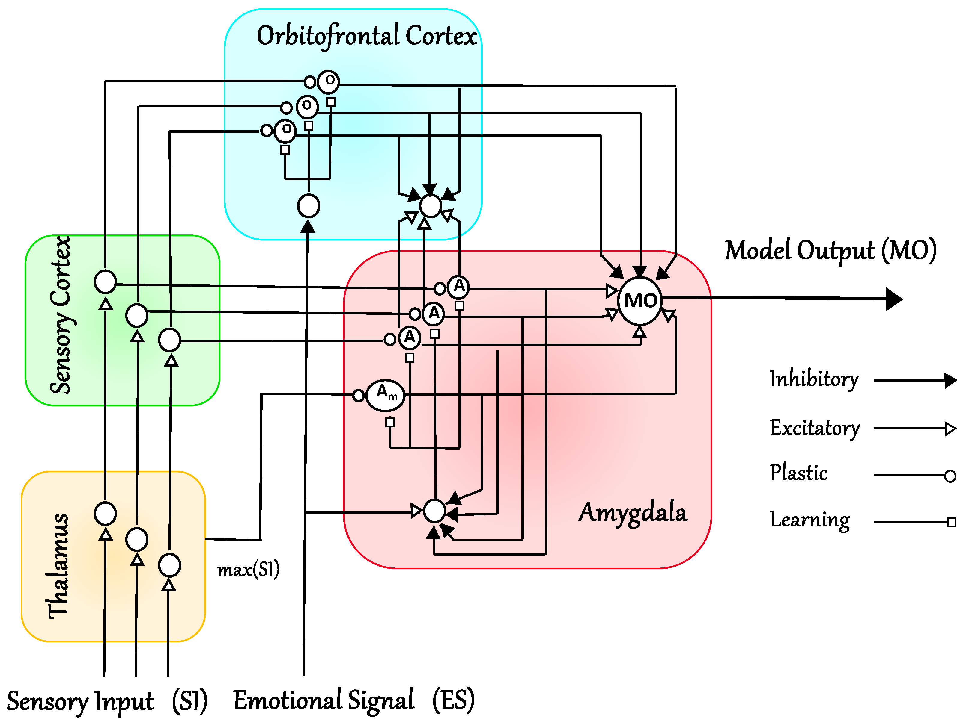
2.2. Brain Emotional Learning

Brain Emotional Learning (BEL) is an intelligent methodology inspired by neurobiology [19,20,21]. The BEL technique is developed based on the mathematical model of the emotional learning process determined in the mammalian limbic system [19,20]. Our adaptation builds upon the network model devised by Moren and Balkenius [20] which emulates key regions such as the amygdala, orbitofrontal cortex, thalamus, sensory input cortex, and other pertinent areas associated with emotional processing. The BEL model utilized in this work, illustrated in Figure 2, comprises the orbitofrontal cortex and amygdala as its two primary components. Essentially, BEL serves as a mechanism for generating actions based on sensory inputs and emotional signals. The amygdala handles immediate learning, whereas the orbitofrontal cortex performs inhibitory actions to suppress any inappropriate learning occurring in the amygdala. Notably, the amygdala lacks the ability to unlearn any previously acquired emotional responses, highlighting the orbitofrontal cortex’s responsibility in inhibiting inappropriate reactions. The BEL model receives two pivotal external inputs: namely, emotional signal (ES) and sensory input (SI) [20,21,28,29].

The output of the BEL model ($MO$) can be characterized as in Equation (9) which is determined by the disparity between the outputs of the amygdala ($A_i$) and the orbitofrontal cortex ($O_i$) nodes.

$$MO=\sum _i{A}_i-\sum _i{O}_i$$

(9)

Here, i represents the number of sensory inputs. The output of each node in the amygdala and the orbitofrontal cortex is characterized as in Equations (10) and (11), respectively. It is worth noting that the outputs of the amygdala and the orbitofrontal cortex are computed through the summation of their respective nodes.

$$A_i=V_i\times S{I}_i$$

(10)

$$O_i=W_i\times S{I}_i$$

(11)

where $S{I}_i$ represents the $i^{th}$ sensory input, $V_i$ denotes the weight associated with the $i^{th}$ node in the amygdala, and $W_i$ represents the weight related to the $i^{th}$ node in the orbitofrontal cortex. The following equations (i.e., Equations (12) and (13)) are utilized to update $V_i$ and $W_i$, respectively:

$$\Delta V_i=K_v\times S{I}_i\times max\left(0,ES-\sum _i{A}_i\right)$$

(12)

$$\Delta W_i=K_w\times S{I}_i\times \left(MO-ES\right)$$

(13)

where $K_v$ and $K_w$ are the learning rates associated with the amygdala and the orbitofrontal cortex, respectively.

Ultimately, the highest value among all sensory inputs is an additional internal input incorporated into the model. Using $V_{th}$ as the weight and employing an update law in Equation (15) analogous to the one illustrated in Equation (12), this signal is directly transmitted from the thalamus to the amygdala and is defined as in Equation (14).

$$A_{th}=V_{th}\times max\left(S{I}_i\right)$$

(14)

$$\Delta V_{th}=K_{v_{th}}\times max\left(S{I}_i\right)\times max\left(0,ES-\sum _i{A}_i\right)$$

(15)

Various approaches have been employed to adjust the BEL parameters [21,28,29,30]. In this study, we adopted the trial-and-error approach similar to those suggested in the literature [21].

2.3. Brain Emotional Learning for Closed-Loop Control of Autonomous Vehicles

In control systems, intelligent/machine learning-based techniques offer solutions to control problems through either direct or indirect methods. The direct approach involves using the intelligent method as a control block, while the indirect approach utilizes it to determine control parameters. In our study, we employed the BEL model as a control block (direct approach), as shown in Figure 3.

This closed-loop configuration includes key blocks: a Brain Emotional Learning controller block, comprising an Emotional Signal Generator, a Sensory Input Generator, a Brain Emotional Learning model, and a block for the AV dynamic model. The Emotional Signal reflects the system’s affective aspects, while the Sensory Input gathers environmental information. Both inputs are crucial for the BEL model. Essentially, a BEL-based controller selects actions based on its Sensory Input and Emotional Signal. The forms of the Sensory Input and Emotional Signal may include system errors, desired inputs, measured/estimated system outputs, and control inputs. Control objectives like reference tracking and optimal control can be implicitly determined by selecting the appropriate Emotional Signal. For instance, choosing the Emotional Signal can optimize reference tracking, reduce overshoot, or minimize energy expenditure.

Our developed ML-based technique aims to intelligently control AVs used in solar panel cleaning systems, addressing uncertainties, disturbances, and dynamic environments to enhance reference tracking, model uncertainty handling, and disturbance rejection. To achieve this, we designed the Emotional Signal such that an increase in reference tracking error induces a negative emotion (e.g., stress) in the system, signaling unsatisfactory performance. Consequently, the developed controller minimizes the negative emotion to ensure satisfactory system performance. To realize these objectives, for each control input ($u=U_l$ being associated with torques/forces), the $S{I}_l$ and $E{S}_l$ are designed as follows (Equations (16) and (17), respectively):

$$\begin{array}{c}\hfill S{I}_l=K_{l,1}^{SI}{e}_l\left(t\right)+K_{l,2}^{SI}\frac{d{e}_l\left(t\right)}{dt}\end{array}$$

(16)

$$\begin{array}{c}\hfill E{S}_l=K_{l,1}^{ES}{e}_l\left(t\right)+K_{l,2}^{ES}\int e_l\left(t\right)dt+K_{l,3}^{ES}\frac{d{e}_l\left(t\right)}{dt}\end{array}$$

(17)

where l denotes the number of controlling variables. Additionally, $K_{l,1}^{SI}$, $K_{l,2}^{SI}$, $K_{l,1}^{ES}$, $K_{l,2}^{ES}$, and $K_{l,3}^{ES}$ represent positive gains. The $ES$ will influence the system behavior differently by assigning distinct values to these positive gains. In this study, different gains are assigned for each control input ($U_l$, $l=1,2,3$) of the system.

Remark 1. 

In accordance with the BEL theory and with the established formulations for $SI$ and $ES$ denoted by Equations (16) and (17), respectively, it can be shown that there exist positive tuning parameters, $K_v$ and $K_w$, satisfying the following conditions:

A. 

$\left|\left[1-K_v{\left(S{I}_l\right)}^2\right]\right|<1$

B. 

$\left|\left[1-K_w{\left(S{I}_l\right)}^2\right]\right|<1$

These conditions ensure that the estimated weights of the amygdala and the orbitofrontal cortex converge asymptotically to the desired targets.

For further details on the Emotional Learning and BEL-based controller utilized in this study, the readers are directed to [19,20,21,28,29].

3. Results

To assess the effectiveness of the control law detailed in the previous section (i.e., Section 2.2 and Section 2.3), this section presents the outcomes of numerical computer simulations applied to successfully control the AV model introduced in Section 2.1 across three distinct scenarios. Three specific simulation scenarios were examined to assess the performance of the developed controller:

• Scenario I: Maintaining constant trajectories for AV angles and displacement.
• Scenario II: Tracking sinusoidal trajectories to maintain AV angles.
• Scenario III: Preserving AV angles and displacement in the presence of substantial external disturbances.

In the initial scenario (Scenario I), the ML-based controller generates suitable control actions to uphold the AV’s displacement (x) and the angles of the front and rear scissors (${\theta }_1$ and ${\theta }_2$) at constant levels. This endeavor aims to achieve the primary objective of controlling the AV’s end effector, i.e., the position of the table. Subsequently, in Scenario II, the proficiency of the ML-based controller is further analyzed by tracking a nonlinear, time-varying signal. Finally, in Scenario III, the performance of the ML-based controller in trajectory tracking under substantial external disturbances is assessed.

For all numerical analyses, the following platform was utilized: a MacBook Pro (macOS 13.6.4) equipped with a 2.3 GHz Intel Core i5 processor and 16.00 GB of memory. The total simulation duration for all scenarios was set to 20 s.

All the simulations are conducted using the following initial conditions:

$$\begin{array}{cc}\hfill {\mathbf{q}}_{\mathbf{0}}& ={\left[0\frac{\pi }{9}\frac{\pi }{9}\right]}^T\hfill \\ \hfill {\dot{\mathbf{q}}}_{\mathbf{0}}& ={\left[000\right]}^T\hfill \end{array}$$

Table 1. Parameters of the Autonomous Vehicle system.

Symbol	Parameter	Value	Unit
$l_1$	Length of link1	0.3535533906	m
$l_2$	Length of link2	0.3535533906	m
$l_{ee}$	Length of the end effector	1.65	m
$m_0$	Mass of body	50	kg
$m_1$	Mass of link1	1.5	kg
$m_2$	Mass of link2	3	kg
$m_3$	Mass of link3	0.2	kg
$m_4$	Mass of link4	0.2	kg
$m_5$	Mass of link5	0.2	kg
$m_6$	Mass of link6	3	kg
$m_7$	Mass of link7	1.5	kg
$m_{ee}$	Mass of the end effector	20	kg
g	Acceleration due to gravity	9.81	m/s2
a	Length of body	1.35	m
b	Distance between motor 3’s center and the ground	0.5	m
$I_{zz0}$	Moment of inertia of body	$1\times {10}^{-7}$	kg·m2
$I_{zz1}$	Moment of inertia of link1	$9.34\times {10}^{-3}$	kg·m2
$I_{zz2}$	Moment of inertia of link2	$7\times {10}^{-2}$	kg·m2
$I_{zz3}$	Moment of inertia of link3	$1\times {10}^{-7}$	kg·m2
$I_{zz4}$	Moment of inertia of link4	$1\times {10}^{-7}$	kg·m2
$I_{zz5}$	Moment of inertia of link5	$1\times {10}^{-7}$	kg·m2
$I_{zz6}$	Moment of inertia of link6	$7\times {10}^{-2}$	kg·m2
$I_{zz7}$	Moment of inertia of link7	$9.34\times {10}^{-3}$	kg·m2
$I_{zzee}$	Moment of inertia of the end effector	1.6	kg·m2

provides the nominal/estimated parameters of the AV system.

Given that PID stands as the predominant controller in practical engineering applications [22,23] and has been featured in prior research for controlling the AVs [24], the outcomes of the BEL-based controllers developed across all three scenarios are compared with those of PID controllers. It is noteworthy that for a fair assessment, the Emotional Signals ($ESs$) of the BEL-based controllers employ identical parameters to the PID controllers. Each controller undergoes tuning only once, as the aim is to assess the performance of both controllers, maintaining their original settings. In essence, there is no further adjustment of the controllers to accommodate the new system conditions.

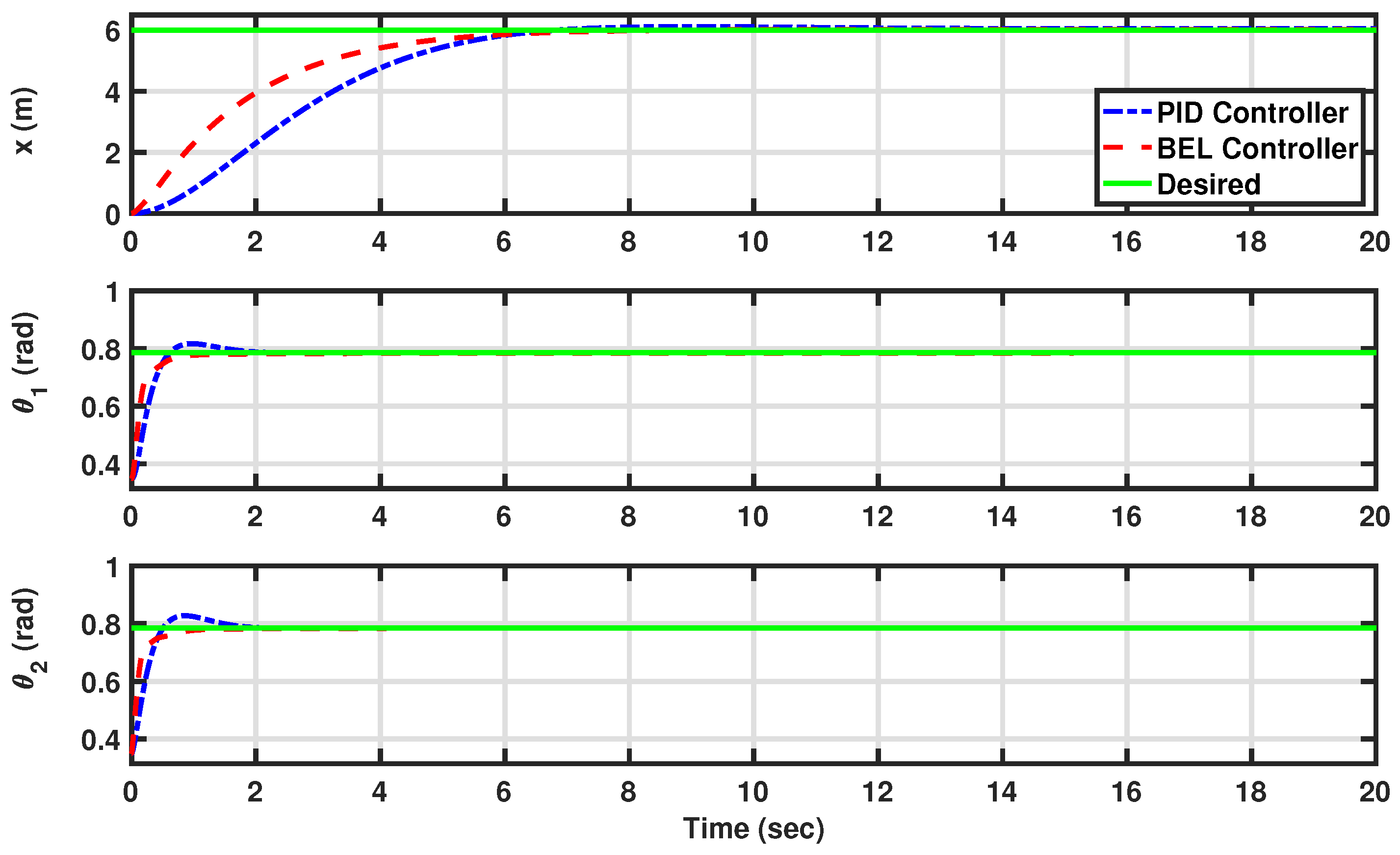
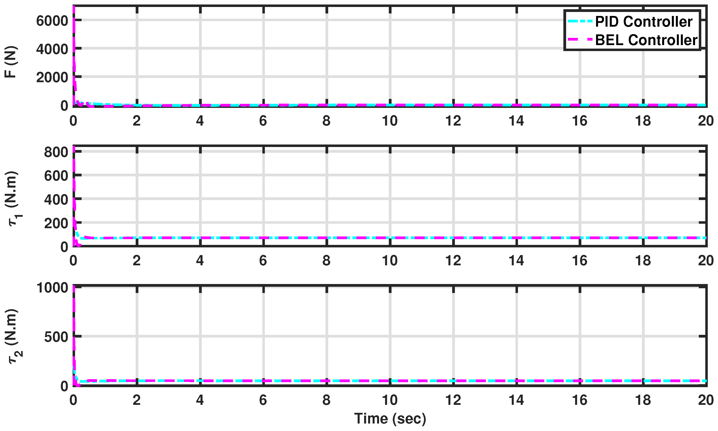
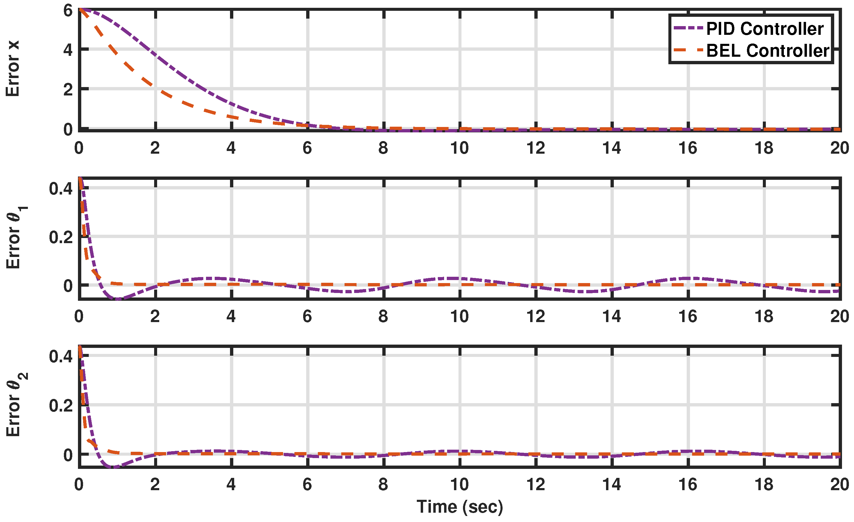
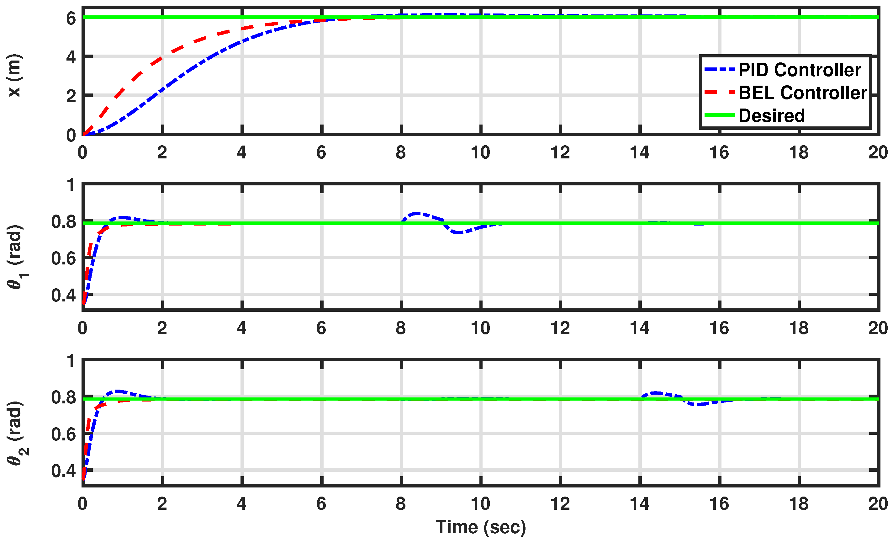
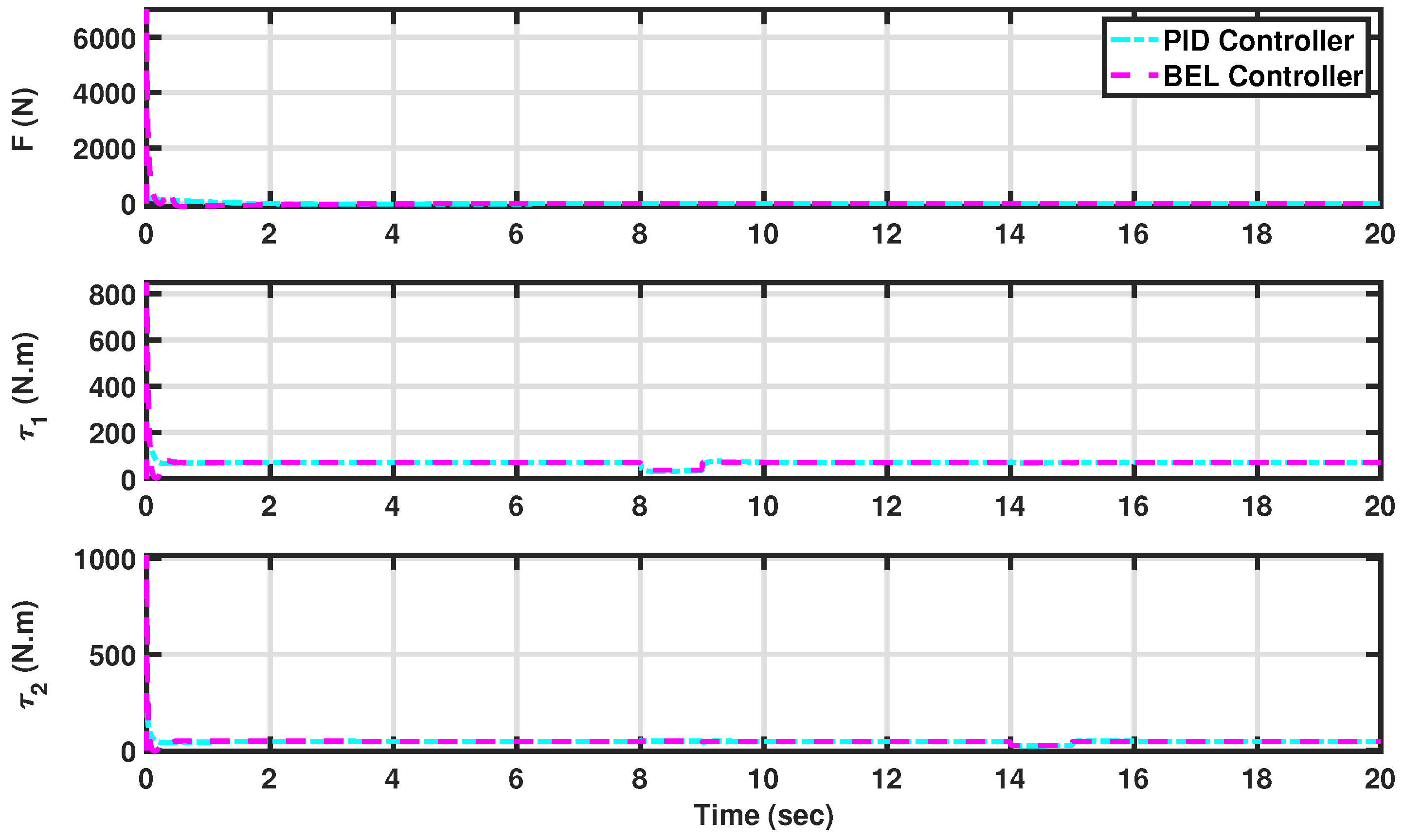
3.1. Scenario I: Maintaining Constant Trajectories for AV’s Angles and Displacement

In the initial scenario (Scenario I), we assess the performance of the developed ML-based controller in preserving the displacement (x) and the angles of the front and rear scissors (${\theta }_1$ and ${\theta }_2$) of the AV at consistent levels. Our focus lies in examining the controller’s ability to generate precise control actions that minimize tracking errors while ensuring a prompt response with minimal overshoot. We define the desired constant trajectories as follows:

$$\begin{array}{cc}\hfill x_d& =6\left[m\right]\hfill \\ \hfill {\theta }_{1_d}& =\frac{\pi }{4}\left[rad\right]\hfill \\ \hfill {\theta }_{2_d}& =\frac{\pi }{4}\left[rad\right]\hfill \end{array}$$

Figure 4 visually compares the desired trajectories with the actual outputs of the controlled system, highlighting the performance under tracking constant trajectories for the initial scenario. Meanwhile, in Figure 5, the control actions generated for the system are depicted, specifically focusing on tracking constant trajectories in Scenario I. Here, the controller developed using BEL is denoted in red with a dashed line, while the PID controller is represented in blue with a dashed–dotted line. Both controllers exhibit efficacy in maintaining the AV system within the desired parameters. Notably, the output under the BEL-based controller showcases faster responses to reference values without overshooting compared to the PID controller, as evidenced in Figure 4. This observation underscores the capability of the developed ML-based controller to regulate the displacement (x) and the angles of the front and rear scissors (${\theta }_1$ and ${\theta }_2$) effectively.

Moreover, Figure 5 provides insight into the smooth and stable nature of the generated control actions, which are crucial for navigating the complex terrain of solar panel arrays and accurately positioning cleaning robots. Here, the BEL-based controller is depicted in magenta with a dashed line, while the PID controller is illustrated in cyan with a dashed–dotted line. The smooth and stable control signals facilitate the seamless movement of the AV, enhancing its operational precision.

To further assess system performance, Figure 6 illustrates the tracking error, contrasting the performance of the BEL-based controller (depicted in orange with a dashed line) against the PID controller (depicted in purple with a dashed–dotted line). This comparison provides valuable insights into the efficacy and robustness of the respective control strategies, aiding in the refinement and optimization of AV systems operating in dynamic environments.

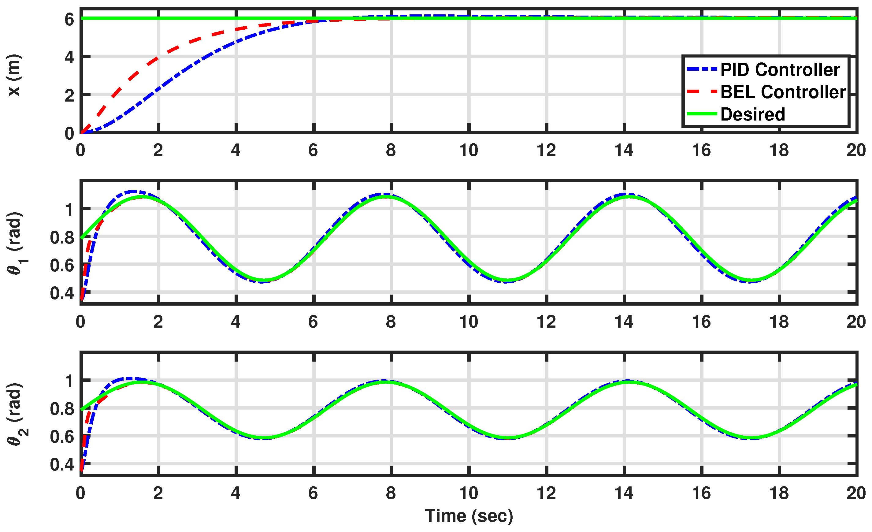
3.2. Scenario II: Tracking Sinusoidal Trajectories to Maintain AV Angles

In the second scenario, denoted as Scenario II, we evaluate the effectiveness of the developed ML-based controller in maintaining the displacement (x) of the AV at a consistent level while simultaneously ensuring that the angles of the front and rear scissors (${\theta }_1$ and ${\theta }_2$) of the AV accurately follow sinusoidal trajectories. Our primary objective is to examine the controller’s capability to generate precise control actions that minimize tracking errors and facilitate a swift response with minimal overshoot. We establish the desired sinusoidal trajectories for the AV’s angles as follows:

$$\begin{array}{cc}\hfill x_d\left(t\right)& =6\left[m\right]\hfill \\ \hfill {\theta }_{1_d}\left(t\right)& =\frac{\pi }{4}+0.3\times sin\left(t\right)\left[rad\right]\hfill \\ \hfill {\theta }_{2_d}\left(t\right)& =\frac{\pi }{4}+0.2\times sin\left(t\right)\left[rad\right]\hfill \end{array}$$

Figure 7 visually compares the desired trajectories with the actual outputs of the controlled system, highlighting the performance under tracking constant/time-varying sinusoidal trajectories for the second scenario. Meanwhile, in Figure 8, the control actions generated for the system are depicted, specifically focusing on maintaining the displacement (x) of the AV at a consistent level while simultaneously ensuring that the angles of the front and rear scissors (${\theta }_1$ and ${\theta }_2$) of the AV accurately follow sinusoidal trajectories as in Scenario II. Here, the controller developed using BEL is denoted in red with a dashed line, while the PID controller is represented in blue with a dashed–dotted line. Both controllers exhibit efficacy in maintaining the AV system within the desired parameters. Notably, the output under the BEL-based controller showcases faster responses to reference values without overshooting compared to the PID controller, as evidenced in Figure 7. This observation underscores the capability of the developed ML-based controller to regulate the displacement (x) at a consistent level while simultaneously ensuring that the angles of the front and rear scissors (${\theta }_1$ and ${\theta }_2$) are accurately following time-varying sinusoidal trajectories effectively.

Moreover, Figure 8 provides insight into the smooth and stable nature of the generated control actions, which is crucial for navigating the complex terrain of solar panel arrays and accurately positioning cleaning robots. Here, the BEL-based controller is depicted in magenta with a dashed line, while the PID controller is illustrated in cyan with a dashed–dotted line. The smooth and stable control signals facilitate the seamless movement of the AV, enhancing its operational precision.

To further assess system performance, Figure 9 illustrates the tracking error, contrasting the performance of the BEL-based controller (depicted in orange with a dashed line) against the PID controller (depicted in purple with a dashed–dotted line). This comparison provides valuable insights into the efficacy, adaptivity, and robustness of the respective control strategies, aiding in the refinement and optimization of AV systems operating in dynamic environments.

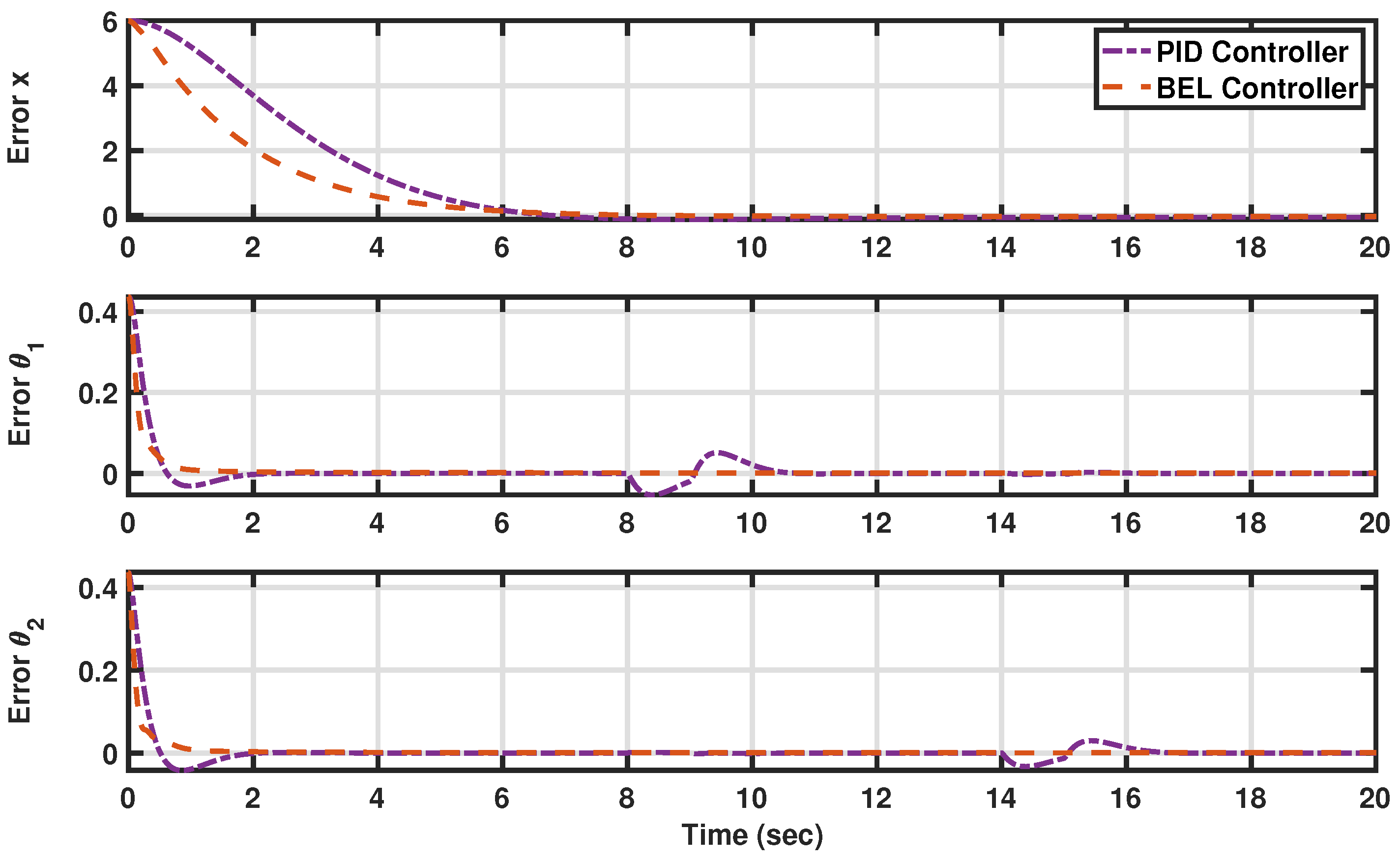
3.3. Scenario III: Preserving AV Angles and Displacement in the Presence of Substantial External Disturbances

Moving on to the final scenario, identified as Scenario III, we investigate the tracking performance of the developed ML-based control approach in the presence of substantial external disturbances. To achieve this, two additional disturbances are introduced to perturb the angles of the front and rear scissors (${\theta }_1={\theta }_1+0.5\times {\theta }_{1_d}$ and ${\theta }_2={\theta }_2+0.5\times {\theta }_{2_d}$) within the time intervals of [8–9] and [14–15] seconds, respectively. In this simulation, we define the desired constant trajectories as follows:

$$\begin{array}{cc}\hfill x_d& =6\left[m\right]\hfill \\ \hfill {\theta }_{1_d}& =\frac{\pi }{4}\left[rad\right]\hfill \\ \hfill {\theta }_{2_d}& =\frac{\pi }{4}\left[rad\right]\hfill \end{array}$$

Figure 10 visually compares the desired trajectories with the actual outputs of the controlled system, highlighting the tracking performance of the developed ML-based control approach in the presence of substantial external disturbances for the last scenario. Meanwhile, in Figure 11, the control actions generated for the system are depicted, specifically focusing on maintaining the displacement (x) of the AV at a consistent level while simultaneously ensuring that the angles of the front and rear scissors (${\theta }_1$ and ${\theta }_2$) of the AV are preserved at consistent levels in the presence of substantial external disturbances as in Scenario III. Here, the controller developed using BEL is denoted in red with a dashed line, while the PID controller is represented in blue with a dashed–dotted line. Both controllers exhibit efficacy in maintaining the AV system within the desired parameters. Notably, the output under the BEL-based controller showcases faster responses to reference values without overshooting compared to the PID controller, as evidenced in Figure 10. Furthermore, compared to the PID controller, the BEL-based controller demonstrates superior performance in handling additional disturbances within the time intervals of [8–9] and [14–15] seconds perturbing the angles of the front and rear scissors.

This observation underscores the capability of the developed ML-based controller to regulate the displacement (x) at a consistent level while simultaneously ensuring that the angles of the front and rear scissors (${\theta }_1$ and ${\theta }_2$) are accurately following their trajectories in the presence of significant external disturbances effectively.

Moreover, Figure 11 provides insight into the smooth and stable nature of the generated control actions, which is crucial for navigating the complex terrain of solar panel arrays and accurately positioning cleaning robots while handling the challenges arising from uncertainties, disturbances, and dynamic environments. Here, the BEL-based controller is depicted in magenta with a dashed line, while the PID controller is illustrated in cyan with a dashed–dotted line. The smooth and stable control signals facilitate the seamless movement of the AV, enhancing its operational precision.

To further assess system performance, Figure 12 illustrates the tracking error, contrasting the performance of the BEL-based controller (depicted in orange with a dashed line) against the PID controller (depicted in purple with a dashed–dotted line). This comparison provides valuable insights into the efficacy, adaptivity, and robustness of the respective control strategies, aiding in the refinement and optimization of AV systems operation by successfully handling the challenges arising from uncertainties, disturbances, and dynamic environments.

4. Discussion and Future Work

The initial examination highlights the efficacy of the introduced ML-based feedback control approach developed using the BEL algorithm. This approach demonstrates its capability to effectively regulate the displacement (x) of the AV and the angles of its front and rear scissors (${\theta }_1$ and ${\theta }_2$) at constant levels, all without requiring prior knowledge of the AV’s dynamics. The findings of this examination are summarized in

Table 2. Rise time, settling time, and overshoot (%) for PID and BEL controllers.

Controller	Rise Time (s)	Settling Time (s)	Overshoot (%)
${\mathbf{PID}}_x$	4.1538	6.3904	1.1553
${\mathbf{BEL}}_x$	3.6840	6.4638	0
${\mathbf{PID}}_{{\theta }_1}$	0.4067	1.4694	3.9919
${\mathbf{BEL}}_{{\theta }_1}$	0.2840	0.7265	0
${\mathbf{PID}}_{{\theta }_2}$	0.3426	1.4541	5.3550
${\mathbf{BEL}}_{{\theta }_2}$	0.1824	0.7780	0

, which provides response specifications demonstrating the superior performance of the developed BEL-based approach. Notably, this superior performance is characterized by a reduced overshoot, faster rise time, and smaller settling time.

Additionally,

Table 3. Percentage Increase/decrease in rise time, settling time, and overshoot (%) using BEL controller.

	Improve (%) Rise Time	Improve (%) Settling Time	Improve (%) Overshoot
x	11.31	$-1.15$	100
${\theta }_1$	30.16	50.56	100
${\theta }_2$	46.76	46.50	100

demonstrates the performance improvements in terms of percentage increase/decrease in the system’s response rise time, settling time, and overshoot (%) using the BEL controller. This further demonstrates the superior performance and efficacy of the ML-based approach, highlighting significant improvements in system responsiveness.

Moving beyond constant trajectory control, the second examination focuses on achieving time-varying sinusoidal trajectory tracking control. Here, the aim is to maintain the AV’s displacement (x) at a consistent level while simultaneously ensuring the accurate tracking of sinusoidal trajectories by the angles of its front and rear scissors (${\theta }_1$ and ${\theta }_2$). In the final examination, attention is turned to evaluating the tracking performance of the developed ML-based control approach in the presence of significant external disturbances. This constitutes a notably challenging task, where achieving faster responses to reference values without overshooting remains a priority.

The findings of these examinations are summarized in

Table 4. Mean-Squared, Root Mean Square, and Mean Absolute Percentage Errors for PID and BEL controllers.

		Scenario I			Scenario II			Scenario III
Controller	MSE	RMSE	MAPE	MSE	RMSE	MAPE	MSE	RMSE	MAPE
${\mathbf{PID}}_x$	3.2878	1.8132	14.1795	3.2879	1.8133	14.1788	3.2878	1.8132	14.1789
${\mathbf{BEL}}_x$	1.8015	1.3422	9.2147	1.8009	1.3419	9.2663	1.8015	1.3422	9.2147
${\mathbf{PID}}_{{\theta }_1}$	0.0017	0.0411	0.8769	0.0022	0.0463	2.9569	0.0018	0.0429	1.4051
${\mathbf{BEL}}_{{\theta }_1}$	0.0009	0.0304	0.7150	0.0009	0.0305	0.6834	0.0009	0.0304	0.7101
${\mathbf{PID}}_{{\theta }_2}$	0.0013	0.0366	0.7964	0.0015	0.0385	1.7258	0.0014	0.0374	1.1238
${\mathbf{BEL}}_{{\theta }_2}$	0.0007	0.0257	0.5639	0.0007	0.0258	0.5362	0.0007	0.0257	0.5623

in terms of the Mean-Squared, Root Mean Square, and Mean Absolute Percentage Errors for both PID and BEL controllers, which provides statistical analysis demonstrating the superior performance of the developed BEL-based approach. Notably, this superior performance is characterized by a significant reduction in tracking errors. This further demonstrates the superior performance and efficacy of the ML-based approach, highlighting significant improvements in system responsiveness and adaptability. These findings underscore the significance of intelligent control strategies in enhancing the operational efficiency of AVs within solar panel cleaning systems, particularly in agricultural solar farms.

Additionally,

Table 5. Percentage increase/decrease in Mean-Squared, Root Mean Square, and Mean Absolute Percentage Errors using BEL controller.

		Scenario I Improve (%)			Scenario II Improve (%)			Scenario III Improve (%)
	MSE	RMSE	MAPE	MSE	RMSE	MAPE	MSE	RMSE	MAPE
x	45.21	25.98	35.01	45.23	25.99	34.65	45.21	25.98	35.01
${\theta }_1$	45.16	25.95	18.46	56.64	34.15	76.89	49.83	29.17	49.46
${\theta }_2$	50.67	29.77	29.19	54.94	32.87	68.93	52.71	31.23	49.97

demonstrates the performance improvements in terms of percentage increase/decrease in the system’s tracking error in Mean-Squared, Root Mean Square, and Mean Absolute Percentage error metrics using the BEL controller. This further demonstrates the superior performance and efficacy of the ML-based approach, highlighting significant improvements in system responsiveness. Upon analyzing these data, it becomes evident that the developed controller consistently yields a more favorable response across various testing scenarios.

Exploring the different future directions, several items could be considered for further investigation. In Section 2, there exists potential for enhancing the current Autonomous Vehicle model (Section 2.1) by designing, improving, and developing an updated model considering more flexibilities in the AV’s mobility.

Since assigning different functions to SI and ES provide design freedom allowing different priorities for control objectives such as minimizing energy expenditure, etc., future work could consider improving the designed ES and SI to achieve optimal performance. In this paper (Section 2.3), priority was given to the simplicity in designing the ES and SI by considering the minimization of the system error while improving the system response and handling system uncertainties and unknown disturbances.

Moreover, while this work assumes the utilization of predefined trajectories generated by higher-level path-planning algorithms, the complex domain of path planning itself warrants further exploration. Therefore, future investigations could delve into path-planning methodologies tailored specifically for Autonomous Vehicles integrated within solar panel cleaning systems [31,32]. Additionally, designing a joint intelligent path planning and control co-design in the presence of system uncertainties and dynamic environment could be considered. This holistic approach seeks to combine path planning and control strategies, optimizing performance and adaptability in real-world scenarios.

Furthermore, future work could consider improving the performance of the developed method as well as providing the experimental results. To do so, first one could consider the analysis of using ML techniques for estimating solar panel performance [33,34]; then, vision-based autonomous navigation and real-time object detection should be considered [35,36].

The exponential growth observed in the electronics industry, coupled with the widespread availability of specialized programming tools and support infrastructure, is driving the accelerated digitization of the agricultural sector including solar panel cleaning systems in agricultural solar farms. Stakeholders in modern agriculture, including farmers and students, are encouraged to familiarize themselves with and actively engage in the development and refinement of innovative systems that enhance agricultural practices [37]. Notably, university students, many of whom possess prior exposure to STEM disciplines, seek real-world experiences to better equip them for their professional endeavors. Bridging this gap, this study could highlight best practices for the various stages of designing, simulating, and implementing Autonomous Vehicles tailored to perform realistic tasks in agricultural settings with a specific focus on solar panel cleaning systems in agricultural solar farms.

Ultimately, the progress in machine learning methods, particularly those deployed in Autonomous Vehicles in agricultural settings via Internet of Things (IoT) devices, might introduce new security risks if awareness and effective countermeasures are not properly implemented [38,39,40,41,42,43]. Therefore, it is essential to address various security challenges when integrating these new techniques.

5. Conclusions

This study investigates the development of an intelligent control system for Autonomous Vehicles (AVs) operating within solar power plants, aiming to address challenges associated with system uncertainties and dynamic environmental conditions. First, the model of the AVs is introduced; then, the computational model of emotional learning in the mammalian limbic system is presented, and finally, the BEL-based controller is developed for the closed-loop control of AVs. Numerical simulations of the AVs controlled by the developed BEL-based method have been illustrated. Through comparative analysis, we demonstrate notable performance improvements compared to conventional PID control methods. In particular, the quantitative results demonstrated the reduced overshoot ($100\%$ improvement in controlling the displacement (x) and the angles of the front and rear scissors (${\theta }_1$ and ${\theta }_2$) of the AV), faster rise time ($11.31\%$ improvement in controlling the displacement (x) and $30.16\%$ and $46.76\%$ for the angles of the front and rear scissors (${\theta }_1$ and ${\theta }_2$) of the AV respectively), and smaller settling time ($50.56\%$ and $46.50\%$ improvement for the angles of the front and rear scissors (${\theta }_1$ and ${\theta }_2$) of the AV, respectively). Additionally, the BEL controller’s results show significant improvement in reducing tracking errors in comparison to the PID controller’s results considering Mean-Squared, Root Mean Square, and Mean Absolute Percentage error metrics. In essence, our findings contribute to the advancement of smart technologies in renewable energy applications, showcasing the efficacy of machine learning techniques in enhancing AV performance for solar panel cleaning tasks. This has significant importance for improving the reliability and efficiency of solar energy systems. We anticipate that our research will stimulate further scientific inquiry in this field to continue optimizing renewable energy infrastructures.

References

1. Amin, A.; Wang, X.; Alroichdi, A.; Ibrahim, A. Designing and Manufacturing a Robot for Dry-Cleaning PV Solar Panels. Int. J. Energy Res. 2023, 2023, 7231554. [Google Scholar] [CrossRef]
2. Akyazi, Ö.; Şahin, E.; Özsoy, T.; Algül, M. A solar panel cleaning robot design and application. Avrupa Bilim Teknol. Derg. 2019, 343–348. [Google Scholar] [CrossRef]
3. De Schepper, E.; Van Passel, S.; Manca, J.; Thewys, T. Combining photovoltaics and sound barriers–A feasibility study. Renew. Energy 2012, 46, 297–303. [Google Scholar] [CrossRef]
4. Dupraz, C.; Marrou, H.; Talbot, G.; Dufour, L.; Nogier, A.; Ferard, Y. Combining solar photovoltaic panels and food crops for optimising land use: Towards new agrivoltaic schemes. Renew. Energy 2011, 36, 2725–2732. [Google Scholar] [CrossRef]
5. Myyas, R.N.; Al-Dabbasa, M.; Tostado-Véliz, M.; Jurado, F. A novel solar panel cleaning mechanism to improve performance and harvesting rainwater. Sol. Energy 2022, 237, 19–28. [Google Scholar] [CrossRef]
6. Jamil, I.; Lucheng, H.; Habib, S.; Aurangzeb, M.; Ahmed, E.M.; Jamil, R. Performance evaluation of solar power plants for excess energy based on energy production. Energy Rep. 2023, 9, 1501–1534. [Google Scholar] [CrossRef]
7. Ghosh, A. Nexus between agriculture and photovoltaics (agrivoltaics, agriphotovoltaics) for sustainable development goal: A review. Sol. Energy 2023, 266, 112146. [Google Scholar] [CrossRef]
8. Thomas, S.K.; Joseph, S.; Sarrop, T.; Haris, S.B.; Roopak, R. Solar panel automated cleaning (SPAC) System. In Proceedings of the 2018 International Conference on Emerging Trends and Innovations In Engineering And Technological Research (ICETIETR), Ernakulam, India, 11–13 July 2018; pp. 1–3. [Google Scholar]
9. Syafiq, A.; Pandey, A.; Adzman, N.; Abd Rahim, N. Advances in approaches and methods for self-cleaning of solar photovoltaic panels. Sol. Energy 2018, 162, 597–619. [Google Scholar] [CrossRef]
10. Kumar, N.M.; Sudhakar, K.; Samykano, M.; Sukumaran, S. Dust cleaning robots (DCR) for BIPV and BAPV solar power plants-A conceptual framework and research challenges. Procedia Comput. Sci. 2018, 133, 746–754. [Google Scholar] [CrossRef]
11. Khadka, N.; Bista, A.; Adhikari, B.; Shrestha, A.; Bista, D. Smart solar photovoltaic panel cleaning system. IOP Conf. Ser. Earth Environ. Sci. 2020, 463, 012121. [Google Scholar] [CrossRef]
12. Hassan, M.U.; Nawaz, M.I.; Iqbal, J. Towards autonomous cleaning of photovoltaic modules: Design and realization of a robotic cleaner. In Proceedings of the 2017 First International Conference on Latest trends in Electrical Engineering and Computing Technologies (INTELLECT), Karachi, Pakistan, 15–16 November 2017; pp. 1–6. [Google Scholar]
13. Khadka, N.; Bista, A.; Adhikari, B.; Shrestha, A.; Bista, D.; Adhikary, B. Current practices of solar photovoltaic panel cleaning system and future prospects of machine learning implementation. IEEE Access 2020, 8, 135948–135962. [Google Scholar] [CrossRef]
14. Deb, D.; Brahmbhatt, N.L. Review of yield increase of solar panels through soiling prevention, and a proposed water-free automated cleaning solution. Renew. Sustain. Energy Rev. 2018, 82, 3306–3313. [Google Scholar] [CrossRef]
15. Saini, A.; Nahar, A.; Yadav, A.K.; Arnim; Shekhawat, D. Solar Panel Cleaning System. Imp. J. Interdiscip. Res. 2017, 3, 26–31. [Google Scholar]
16. Hajiahmadi, F.; Dehghani, M.; Zarafshan, P.; Moosavian, S.A.A.; Hassan-Beygi, S. Trajectory control of a robotic carrier for solar power plant cleaning system. In Proceedings of the 2019 7th International Conference on Robotics and Mechatronics (ICRoM), Tehran, Iran, 20–21 November 2019; pp. 463–468. [Google Scholar]
17. Hajiahmadi, F.; Dehghani, M.; Zarafshan, P.; Moosavian, S.A.A.; Hassan-Beygi, S.R. Initial analysis and development of an automated maintenance system for Agrivoltaics plants. Agric. Eng. Int. CIGR J. 2023, 25, 130–145. [Google Scholar]
18. Jafari, M.; Reyhanoglu, M.; Kozhabek, Z. Simple Learning-Based Robust Nonlinear Control of an Electric Pump for Liquid-Propellant Rocket Engines. Electronics 2023, 12, 3527. [Google Scholar] [CrossRef]
19. LeDoux, J.E. Brain mechanisms of emotion and emotional learning. Curr. Opin. Neurobiol. 1992, 2, 191–197. [Google Scholar] [CrossRef] [PubMed]
20. Morén, J.; Balkenius, C. A computational model of emotional learning in the amygdala. Anim. Animat. 2000, 6, 115–124. [Google Scholar]
21. Lucas, C.; Shahmirzadi, D.; Sheikholeslami, N. Introducing BELBIC: Brain emotional learning based intelligent controller. Intell. Autom. Soft Comput. 2004, 10, 11–21. [Google Scholar] [CrossRef]
22. Johnson, M.A.; Moradi, M.H. PID Control; Springer: Berlin/Heidelberg, Germany, 2005. [Google Scholar]
23. Wang, L. PID Control System Design and Automatic Tuning Using MATLAB/Simulink; John Wiley & Sons: Hoboken, NJ, USA, 2020. [Google Scholar]
24. Hajiahmadi, F.; Zarafshan, P.; Dehghani, M.; Moosavian, S.A.A.; Hassan-Beygi, S. Dynamics modeling and position control of a robotic carrier for solar panel cleaning system. In Proceedings of the 2019 7th International Conference on Robotics and Mechatronics (ICRoM), Tehran, Iran, 20–21 November 2019; pp. 613–618. [Google Scholar]
25. Spong, M.W.; Hutchinson, S.; Vidyasagar, M. Robot Modeling and Control; John Wiley & Sons: Hoboken, NJ, USA, 2020. [Google Scholar]
26. Craig, J.J. Introduction to Robotics; Pearson Educacion: London, UK, 2006. [Google Scholar]
27. Hajiahmadi, F.; Zarafshan, P.; Dehghani, M.; Moosavian, S.A.A.; Hassanbeigi, R. Dynamic modeling and control of cleaning robot for agro-photovoltaic. Amirkabir J. Mech. Eng. 2021, 53, 3465–3478. [Google Scholar]
28. Jafari, M.; Xu, H.; Carrillo, L.R.G. Brain emotional learning-based path planning and intelligent control co-design for unmanned aerial vehicle in presence of system uncertainties and dynamic environment. In Proceedings of the 2018 IEEE Symposium Series on Computational Intelligence (SSCI), Bangalore, India, 18–21 November 2018; pp. 1435–1440. [Google Scholar]
29. Jafari, M.; Xu, H. Biologically-inspired intelligent flocking control for networked multi-UAS with uncertain network imperfections. Drones 2018, 2, 33. [Google Scholar] [CrossRef]
30. Jafari, M.; Shahri, A.M.; Elyas, S.H. Optimal tuning of brain emotional learning based intelligent controller using clonal selection algorithm. In Proceedings of the ICCKE 2013, Mashhad, Iran, 31 October–1 November 2013; pp. 30–34. [Google Scholar]
31. Ghobadpour, A.; Monsalve, G.; Cardenas, A.; Mousazadeh, H. Off-road electric vehicles and autonomous robots in agricultural sector: Trends, challenges, and opportunities. Vehicles 2022, 4, 843–864. [Google Scholar] [CrossRef]
32. Karunathilake, E.; Le, A.T.; Heo, S.; Chung, Y.S.; Mansoor, S. The path to smart farming: Innovations and opportunities in precision agriculture. Agriculture 2023, 13, 1593. [Google Scholar] [CrossRef]
33. Dobrilovic, D.; Pekez, J.; Ognjenovic, V.; Desnica, E. Analysis of Using Machine Learning Techniques for Estimating Solar Panel Performance in Edge Sensor Devices. Appl. Sci. 2024, 14, 1296. [Google Scholar] [CrossRef]
34. Tilahun, F.B. Machine learning interfaces for modular modelling and operation-based design optimization of solar thermal systems in process industry. Eng. Appl. Artif. Intell. 2024, 127, 107285. [Google Scholar] [CrossRef]
35. Rodriguez-Vazquez, J.; Prieto-Centeno, I.; Fernandez-Cortizas, M.; Perez-Saura, D.; Molina, M.; Campoy, P. Real-Time Object Detection for Autonomous Solar Farm Inspection via UAVs. Sensors 2024, 24, 777. [Google Scholar] [CrossRef] [PubMed]
36. Xu, S.; Rai, R. Vision-based autonomous navigation stack for tractors operating in peach orchards. Comput. Electron. Agric. 2024, 217, 108558. [Google Scholar] [CrossRef]
37. Loukatos, D.; Kondoyanni, M.; Kyrtopoulos, I.V.; Arvanitis, K.G. Enhanced robots as tools for assisting agricultural engineering students’ development. Electronics 2022, 11, 755. [Google Scholar] [CrossRef]
38. Yazdinejad, A.; Zolfaghari, B.; Azmoodeh, A.; Dehghantanha, A.; Karimipour, H.; Fraser, E.; Green, A.G.; Russell, C.; Duncan, E. A review on security of smart farming and precision agriculture: Security aspects, attacks, threats and countermeasures. Appl. Sci. 2021, 11, 7518. [Google Scholar] [CrossRef]
39. Bui, H.T.; Aboutorab, H.; Mahboubi, A.; Gao, Y.; Sultan, N.H.; Chauhan, A.; Parvez, M.Z.; Bewong, M.; Islam, R.; Islam, Z.; et al. Agriculture 4.0 and Beyond: Evaluating Cyber Threat Intelligence Sources and Techniques in Smart Farming Ecosystems. Comput. Secur. 2024, 140, 103754. [Google Scholar] [CrossRef]
40. Yazdinejad, A.; Dehghantanha, A.; Karimipour, H.; Srivastava, G.; Parizi, R.M. An efficient packet parser architecture for software-defined 5g networks. Phys. Commun. 2022, 53, 101677. [Google Scholar] [CrossRef]
41. Rudrakar, S.; Rughani, P. IoT based agriculture (Ag-IoT): A detailed study on architecture, security and forensics. Inf. Process. Agric. 2023. Available online: https://www.sciencedirect.com/science/article/pii/S2214317323000665?via%3Dihub (accessed on 16 April 2024).
42. Yazdinejad, A.; Dehghantanha, A.; Srivastava, G.; Karimipour, H.; Parizi, R.M. Hybrid privacy preserving federated learning against irregular users in Next-generation Internet of Things. J. Syst. Archit. 2024, 148, 103088. [Google Scholar] [CrossRef]
43. Fathy, C.; Ali, H.M. A secure IoT-based irrigation system for precision agriculture using the expeditious cipher. Sensors 2023, 23, 2091. [Google Scholar] [CrossRef] [PubMed]
Figure 1. Autonomous Vehicle utilized for carrying and positioning cleaning robots in solar panel cleaning systems.
Agriengineering 06 00081 g001
Figure 2. Graphical schematic depicting the mathematical model of Brain Emotional Learning (BEL) in the mammalian limbic system.
Agriengineering 06 00081 g002
Figure 3. Brain Emotional Learning controller architecture for closed-loop control of Autonomous Vehicles.
Agriengineering 06 00081 g003
Figure 4. The desired and actual outputs of the system [the displacement (x) and the angles of the front and rear scissors ( θ 1 and θ 2 )] in constant trajectory tracking (see Scenario I: Maintaining constant trajectories for AV angles and displacement). The developed BEL-based controller is in red (dashed line), the PID is in blue (dashed–dotted line), and the desired trajectories are in green (solid line).
Agriengineering 06 00081 g004
Figure 5. The generated forces and torques by both controllers in constant trajectory tracking (see Scenario I: Maintaining constant trajectories for AV angles and displacement). The developed BEL-based controller is in magenta (dashed line), and the PID is in cyan (dashed–dotted line).
Agriengineering 06 00081 g005
Figure 6. The tracking errors in constant trajectory tracking (see Scenario I: Maintaining constant trajectories for AV angles and displacement). The developed BEL-based controller is in orange (dashed line), and the PID is in purple (dashed–dotted line).
Agriengineering 06 00081 g006
Figure 7. The desired and actual outputs of the system [the displacement (x) and the angles of the front and rear scissors ( θ 1 and θ 2 )] in tracking constant/time-varying sinusoidal trajectories (see Scenario II: Tracking sinusoidal trajectories to maintain AV angles). The developed BEL-based controller is in red (dashed line), the PID is in blue (dashed–dotted line), and the desired trajectories are in green (solid line).
Agriengineering 06 00081 g007
Figure 8. The generated forces and torques by both controllers in tracking constant/time-varying sinusoidal trajectories (see Scenario II: Tracking sinusoidal trajectories to maintain AV angles). The developed BEL-based controller is in magenta (dashed line) and the PID is in cyan (dashed–dotted line).
Agriengineering 06 00081 g008
Figure 9. The tracking errors in tracking constant/time-varying sinusoidal trajectories (see Scenario II: Tracking sinusoidal trajectories to maintain AV angles). The developed BEL-based controller is in orange (dashed line), and the PID is in purple (dashed–dotted line).
Agriengineering 06 00081 g009
Figure 10. The desired and actual outputs of the system [the displacement (x) and the angles of the front and rear scissors ( θ 1 and θ 2 )] in tracking trajectories in the presence of substantial external disturbances (see Scenario III: Preserving AV angles and displacement in the presence of substantial external disturbances). External disturbances are introduced to perturb the angles of the front and rear scissors within the time intervals of [8–9] and [14–15] seconds, respectively. The developed BEL-based controller is in red (dashed line), the PID is in blue (dashed–dotted line), and the desired trajectories are in green (solid line).
Agriengineering 06 00081 g010
Figure 11. The generated forces and torques by both controllers in tracking trajectories in the presence of substantial external disturbances (see Scenario III: Preserving AV angles and displacement in the presence of substantial external disturbances). The developed BEL-based controller is in magenta (dashed line), and the PID is in cyan (dashed–dotted line).
Agriengineering 06 00081 g011
Figure 12. The tracking errors in tracking trajectories in the presence of substantial external disturbances (see Scenario III: Preserving AV angles and displacement in the presence of substantial external disturbances). The developed BEL-based controller is in orange (dashed line), and the PID is in purple (dashed–dotted line).
Agriengineering 06 00081 g012