Abstract
In arid and semiarid regions, crop production has high irrigation water demands due to low precipitation. Efficient irrigation water management strategies can be developed using crop growth models to assess the effect of different irrigation management practices on crop productivity. The leaf area index (LAI) is an important growth parameter used in crop modeling. Measuring LAI requires specialized and expensive equipment not readily available for producers. Canopy cover (CC) and canopy height (CH) measurements, on the other hand, can be obtained with little effort using mobile devices and a ruler, respectively. The objective of this study was to determine the relationships between LAI, CC, and CH for fully and deficit-irrigated alfalfa (Medicago sativa L.). The LAI, CC, and CH measurements were obtained from an experiment conducted at the Valley Road Field Lab in Reno, Nevada, starting in the Fall of 2020. Three irrigation treatments were applied to two alfalfa varieties (Ladak II and Stratica): 100%, 80%, and 60% of full irrigation demands. Biweekly measurements of CC, CH, and LAI were collected during the growing seasons of 2021 and 2022. The dataset was randomly split into training and testing subsets. For the training subset, an exponential model and a simple linear regression (SLR) model were used to determine the individual relationship of CC and CH with LAI, respectively. Also, a multiple linear regression (MLR) model was implemented for the estimation of LAI with CC and CH as its predictors. The exponential model was fitted with a residual standard error (RSE) and coefficient of determination (R2) of 0.97 and 0.86, respectively. A lower performance was obtained for the SLR model (RSE = 1.03, R2 = 0.81). The MLR model (RSE = 0.82, R2 = 0.88) improved the performance achieved by the exponential and SLR models. The results of the testing indicated that the MLR performed better (RSE = 0.82, R2 = 0.88) than the exponential model (RSE = 0.97, R2 = 0.86) and the SLR model (RSE = 1.03, R2 = 0.82) in the estimation of LAI. The relationships obtained can be useful to estimate LAI when CC, CH, or both predictors are available and assist with the validation of data generated by crop growth models.
1. Introduction
The leaf area index (LAI) is an important measure that controls the physical and biological processes of plant canopies [1]. It is defined as the unitless ratio of one-sided leaf area per unit ground area. The literature reports that the LAI of alfalfa (Medicago sativa L.) is closely related to yield [2,3]. Therefore, plant breeders select plants with larger leaf areas to increase yield. Nelson and Smith [4] attributed a higher radiant energy conversion into dry matter in alfalfa to its higher LAI when compared to birdsfoot trefoil (Lotus corniculatus L.) at similar net assimilation rates. Bolger and Matches [5] found that differences in LAI accounted for differences in evapotranspiration between sainfoin (Onobrychis viciifolia Scop.) and alfalfa. According to Greub and Wedin [6], the LAI values needed to initiate a net accumulation of total nonstructural carbohydrate (TNC) in alfalfa roots were 2.4 for spring growth and 1.6, 0.8, and 1.8 for regrowth following the first, second, and third cuttings, respectively. Afsharmanesh [7] reported that the LAI was reduced with the increase in the intensity of drought stress, and dry forage had a high correlation with LAI. Rimi et al. [8] found a positive correlation between the LAI to stem area index and forage nutritive value.
Canopy cover (CC) is defined as the area of the ground covered by a vertical projection of the canopy. It is an essential diagnostic parameter for estimating canopy development, light interception, stage of growth, evapotranspiration partitioning, and crop water use [9,10]. Digital image analysis (DIA) is a method used to estimate CC. Xiong et al. [11] compared two DIA programs for ground cover estimation, their capability to estimate canopy functions, and the time reduction for vegetation analysis compared to a manual method in pastures of Old World bluestem [Bothriochloa bladhii (Retz) Blake]. When using CC estimated from DIA methods, it was found that the time required to estimate photosynthetic active radiation interception, LAI, and green biomass was reduced to 3.6% of manual methods. Baxter et al. [12] used the DIA to estimate available forage in alfalfa-tall wheatgrass pasture (R2 of calibration model = 0.66), finding promising results in non-destructive estimation. Currently, with the Canopeo app developed by Patrignani and Ochsner [9], fractional green canopy cover (FGCC) in images and videos can be rapidly and accurately measured using a mobile device, making CC estimation accessible to farmers.
Crop growth models such as the Decision Support System for Agrotechnology Transfer (DSSAT) [13] and the Agricultural Production Systems SIMulator (APSIM) [14] model the canopy expansion of crops. These crop growth models require input datasets consisting of agronomic indicators of crop development measured in the field, such as LAI, to validate the results of their simulations. This agronomic indicator can be estimated in a non-destructive way using a canopy analyzer (LAI-2200C, LI-COR, Lincoln, NE) that uses a radiative transfer model to calculate LAI from measurements of intercepted solar radiation. However, the estimation of LAI is not accessible to most farmers due to the expensive cost of this device.
Crop growth models can be used to evaluate different deficit irrigation strategies (defined as the practice of irrigating a crop without meeting its full water demands) to ameliorate the yield decrease caused by water stress [15,16,17,18,19]. Periodic data assimilation of key agronomic indicators can improve the outcomes of crop growth models. Linker and Kisekka [20] found that weekly measurements of LAI fed to a crop growth model allowed the model to achieve an overall performance (quantified as yield vs. irrigation amount) that was within 3% of the performance achieved by a benchmark model.
Hence, there is a need for mathematical models that can facilitate the estimation of alfalfa LAI from other agronomic indicators of crop development, such as CC and CH, whose estimation and measurement, respectively, are accessible to most farmers. With these mathematical functions, LAI can be quickly and inexpensively estimated from digital photographs of CC taken with a mobile device with an RGB camera or from CH measurements. This study aims to determine the numerical relationships between LAI, CC, and CH for fully and deficit-irrigated alfalfa.
Previous studies have found a relationship between the LAI and CC for different crops. Nielsen et al. [21] determined an exponential relationship between the LAI and CC for corn (R2 = 0.97), winter wheat (R2 = 0.96), and spring triticale (R2 = 0.90) under dryland and limited irrigation conditions. Córcoles et al. [22] analyzed the relationship between LAI and CC in onion, fitting a linear (R2 = 0.84), a polynomial (R2 = 0.84), and an exponential model (R2 = 0.75), obtaining better results with the linear and polynomial models. Liu and Pattey [23] reported a logarithmic model (R2 = 0.83) for the LAI estimation of corn, soybean, and wheat from vertical gap fraction measurements obtained using top-of-canopy digital color photography. Other studies estimated the LAI using CH as its predictor. Labbafi et al. [24] used a linear model to estimate the LAI of pumpkins as a function of CH (R2 between 0.91 and 0.93). Logsdon and Cambardella [25] determined the LAI of corn, soybean, oat, alfalfa, and a perennial mixed forage combining CC and CH for two continuous growing seasons, with an R2 ranging from 0.43 to 0.69. In a recent study, Hammond et al. [26] estimated LAI in alfalfa with a simple linear regression (SLR) model of different visible vegetation indices and with a multiple linear regression (MLR) model using the visible vegetation indices and CH as the predictors. The prediction of LAI improved with the addition of CH to the MLR model (R2 = 0.93). However, the requirement of an unmanned aerial vehicle with an RGB camera to collect the imagery and derive the vegetation indices limits the utilization of these models by farmers. Therefore, there is still a need to find simple numerical relationships that allow farmers to estimate LAI without the need to use expensive equipment. We hypothesize that the LAI of full and deficit-irrigated alfalfa can be accurately estimated as a function of CC and that the prediction of LAI can be improved by including CH as an additional predictor. Hence, the specific objective of this study is to develop models that can be used to estimate alfalfa LAI using CC and CH as predictors.
2. Materials and Methods
2.1. Field Experiment
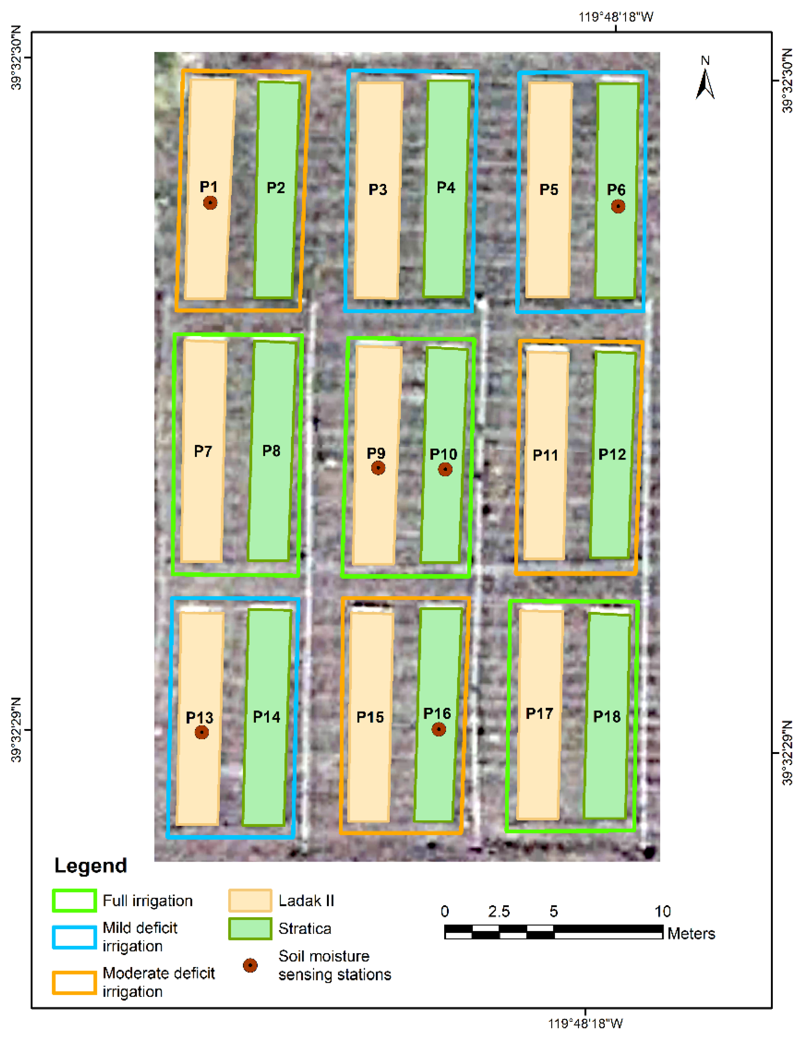
The experiment was conducted in Reno, Nevada, at the University of Nevada, Reno’s Valley Road Field Laboratory (39°32′29.42″ N, 119°48′18.09″ W, 1370 m above sea level), during the summer growing seasons of 2021 and 2022 using a drip irrigation system. The study area has a cold semi-arid climate (Köppen: BSk) with total annual precipitation, snowfall, reference evapotranspiration (ETo), and average air temperature of 186.7 mm, 530.9 mm, 1373.3 mm, and 12.8 °C, respectively. The daily meteorological variables were measured by a weather station located at the Valley Road Field Laboratory that reports data to the Western Regional Climate Center (Table 1) [27]. The experimental design was a strip plot, with three irrigation treatment levels (100%, 80%, and 60% of replenishment of soil water depletion to field capacity in the top 1.5 m of soil) as the whole plots, two alfalfa varieties (Ladak II, Great Basin Seeds, Ephraim, UT and Stratica, Croplan, Arden Hills, MN, USA) as the whole plots orthogonal to the original plots used for the irrigation factor, and three replications (Figure 1). Alfalfa was sown in September 2020 in plots with dimensions of 9.14 m long and 1.63 m wide. The soil of the experimental site is classified as a Fleishmann gravelly clay loam with 2 to 4 percent slopes [28].

Table 1.
Monthly average air temperature, solar radiation, and precipitation during the growing seasons of 2021 and 2022.

Figure 1.
Experimental layout with the full irrigation (FI), mild deficit irrigation (80% of FI), and moderate deficit irrigation (60% of FI) treatments, and the two alfalfa varieties (Ladak II and Stratica).
2.2. Imagery Acquisition
A multispectral camera (Tetracam ADC; Tetracam Inc., Chatsworth, CA) was used to acquire the data every two weeks during the growing seasons of 2021 and 2022 (Table 2). Before each data collection, the calibration target was placed on the ground, and an image was taken for calibration purposes. Then, the camera was attached to a frame, and the Bluetooth module was connected to the camera. The frame was placed next to the plot to put the camera directly above alfalfa rows at a nadir position (Figure 2). The camera was remotely triggered with the S_Link App version 2.6, taking pictures inside the south, middle, and north portions of each plot for a total of three pictures per plot.
Table 2.
Tetracam ADC multispectral camera specifications.
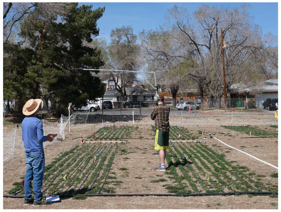
Figure 2.
Multispectral camera attached to frame to acquire images. Pictures were collected inside the south, middle, and north portions of each plot, for a total of three pictures per plot.
2.3. Canopy Cover (CC) and Canopy Height (CH)
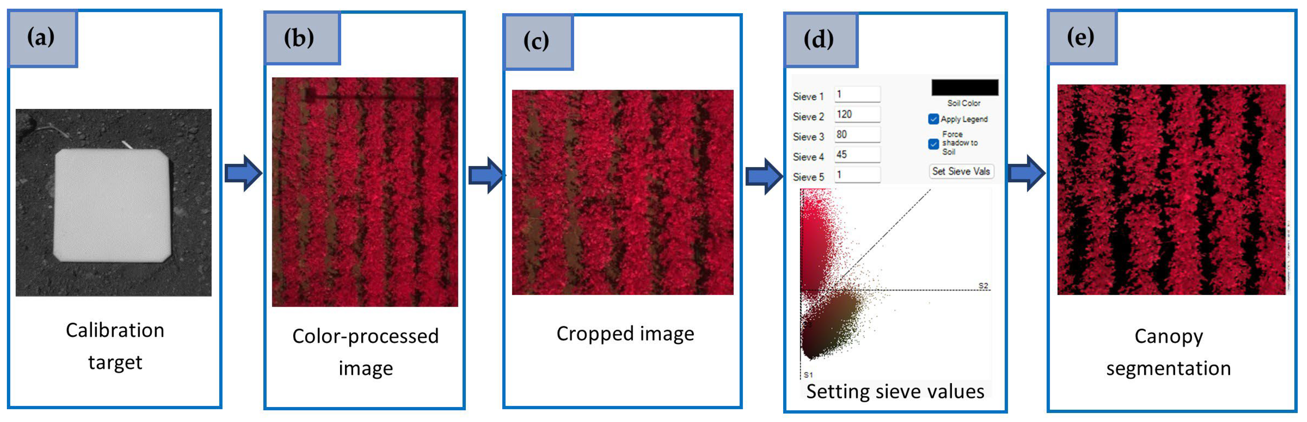
The software PixelWrench2 version 1.2.4.7 was used to process the images. Each image of the calibration target was opened in PixelWrench2, and an area in the center was selected to create a color profile (*.cpf) file on the Matrix page of the Index Tools (Figure 3a). Then, each set of images was color-processed using the corresponding *.cpf file (Figure 3b). Color-processed images were cropped to a resolution of 1250 × 1250 pixels to remove the border effect using a custom script developed in the Python programming language (Figure 3c). An image from each set of cropped images was selected to set the sieve values in the canopy page by selecting areas of the image occupied by soil and vegetation (Figure 3d). In the Batch page, the canopy segmentation was chosen to process each set of images to differentiate between vegetation pixels and background pixels and obtain the percentage of the image covered by vegetation (Figure 3e).

Figure 3.
Image processing to obtain the canopy cover. Calibration target used for the radiometric correction (a), color-processed images after calibration (b), cropped image showing internal rows (c), sieve values used to classify image based on the red and near-infrared reflectance of the soil (d), and canopy cover (e).
Canopy height (CH) was measured every two weeks to monitor plant growth. Two quadrats with an area of one square meter were delimited in each plot. Then, three random plants were selected in each quadrat to measure the CH at the beginning, middle, and end of the internal rows within each quadrat using a meter stick. Therefore, in each plot, a total of six measurements were collected, and the averages were reported.
2.4. Leaf Area Index (LAI) Data Collection
Leaf area index (LAI) was measured with a LAI-2200C (LI-COR, Lincoln, NE, USA) on a biweekly basis. The measurements were collected on the same days and locations when and where the imagery data were collected with the multispectral camera. Readings to measure the sky radiation properties were made before logging below-canopy readings. Both above and below readings were collected without a view cap, but the same portion of the sensor field of view was blocked by the operator. FV2200 software version 2.1.1 was used to save the data stored by the instrument. The LAI values were measured inside the south, middle, and north portions of each plot. The average of these three LAI values was calculated and reported as the LAI of the plot.
2.5. Model Fitting and Evaluation
An exploratory analysis was performed in the R environment, version 4.2.1 [29]. It involved boxplot generation, determination of the correlation between the variables, visualization of the histograms, and scatterplots relating CC and CH with LAI. The dataset was randomly split into a training and testing subset with the sample.split function of the caTools package [30] using a split ratio of 80% of the data for training and 20% for testing (Figure 4). The scatterplot of CC and LAI suggested that fitting an exponential model was appropriate. Therefore, an exponential model was fitted to the training set with CC as the predictor using the nls function (Nonlinear Least Squares) of the stats package. Also, a simple linear regression (SLR) of LAI as a function of CH was fitted with the lm function in R considering the relationship suggested by the scatterplot of CH and LAI. Similarly, a multiple linear regression (MLR) model of LAI that contained both CC and CH was implemented to determine if the prediction of LAI could improve by including both predictors in the same model.
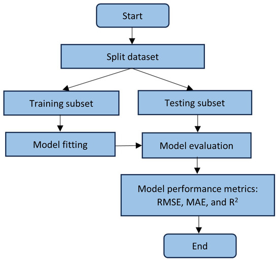
Figure 4.
Flowchart showing the main steps followed to fit the models and their evaluation.
Testing of the models was performed using the predict function in R, and the model performance metrics root mean square error (RMSE) (Equation (1)), mean absolute error (MAE) (Equation (2)), and R2 were calculated.
where:
Pi = predicted value.
Oi = observed value.
n = number of observations.
2.6. Analysis of Variance
According to the fixed and random effects in the experiment, a repeated measures linear mixed-effects model was fitted to the LAI, CC, and CH, considering the response variables by date of collection as the repeated measures. The model included a three-way interaction of irrigation treatment, variety, and date of collection with a random intercept of the experimental unit. When the effect was statistically significant (p < 0.05), the difference between means was evaluated for significance using Tukey’s Honest Significance Difference (HSD) test.
3. Results
The descriptive statistics of CC, CH, and LAI are presented in Table 3. In the 2021 season, the lowest mean CC, LAI, and CH values were obtained on 23 July (8 days after the second harvest period). In contrast, the highest mean LAI and CH values were measured on 1 June (14 days before the first harvest period). The highest mean CC during this season was observed on 22 September (1 day before the fourth harvest period). In the season 2022, the lowest mean CC and LAI were obtained on 8 April (61 days before the first harvest period). The lowest mean CH was measured on 23 June (15 days before the fourth harvest period). Meanwhile, the highest mean CC, LAI, and CH were measured on 7 June (1 day before the first harvest period).
Table 3.
Descriptive statistics of canopy cover (CC), canopy height (CH), and leaf area index (LAI), as well as harvest dates during the 2021 and 2022 growing seasons.
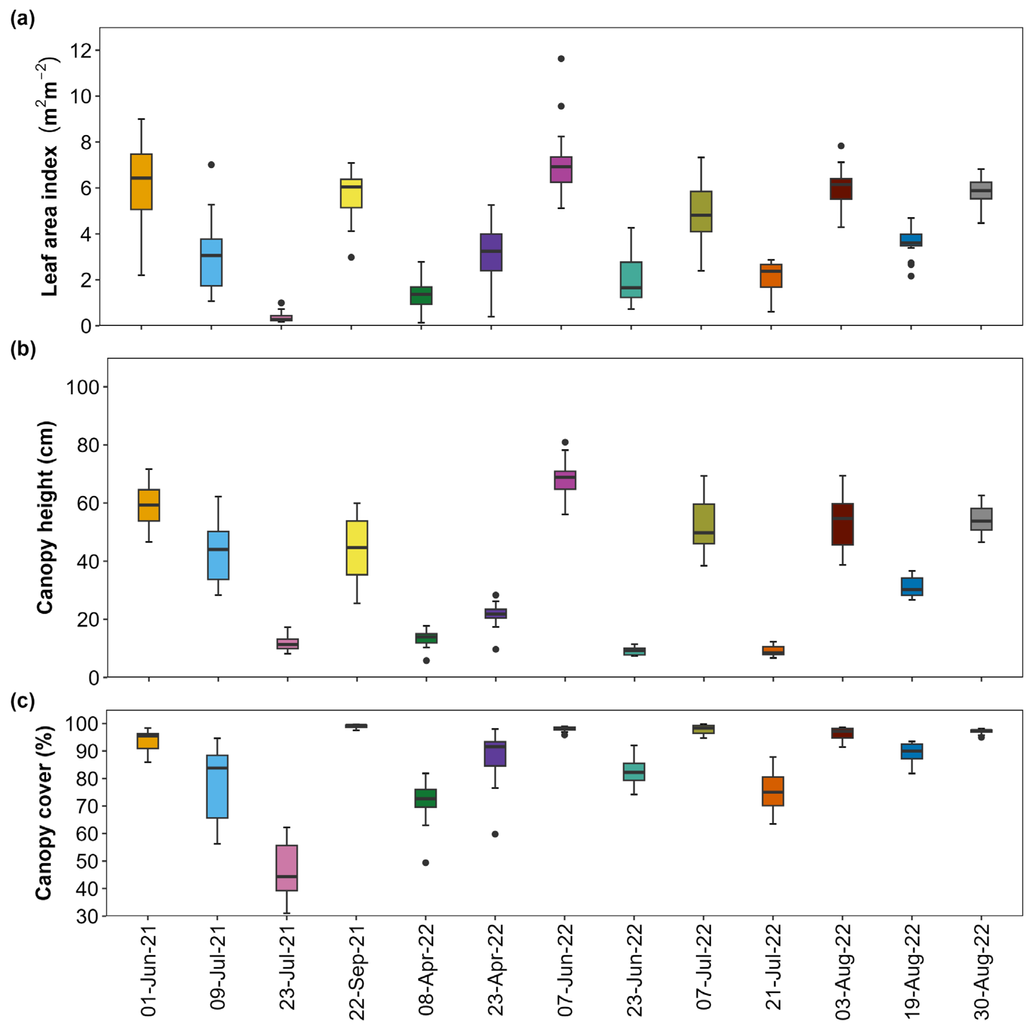
The highest variability in the LAI was observed on 1 June 2021, with a negatively skewed distribution (Figure 5a). In the case of CH and CC, the highest variability occurred on 9 July 2021 (6 days before the second harvest period), with a negatively skewed distribution (Figure 5b,c). The LAI, CH, and CC followed the same trend throughout the two growing seasons, with higher values before each harvest and lower values at the start of the growing season or in the middle of a harvest period. In both seasons, some outliers were observed in the LAI data. Fewer outliers were found in the CH and CC data during the 2022 growing season.
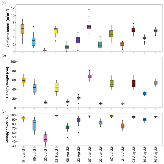
Figure 5.
Box plots of leaf area index (a), canopy height (b), and canopy cover (c) throughout the two growing seasons.
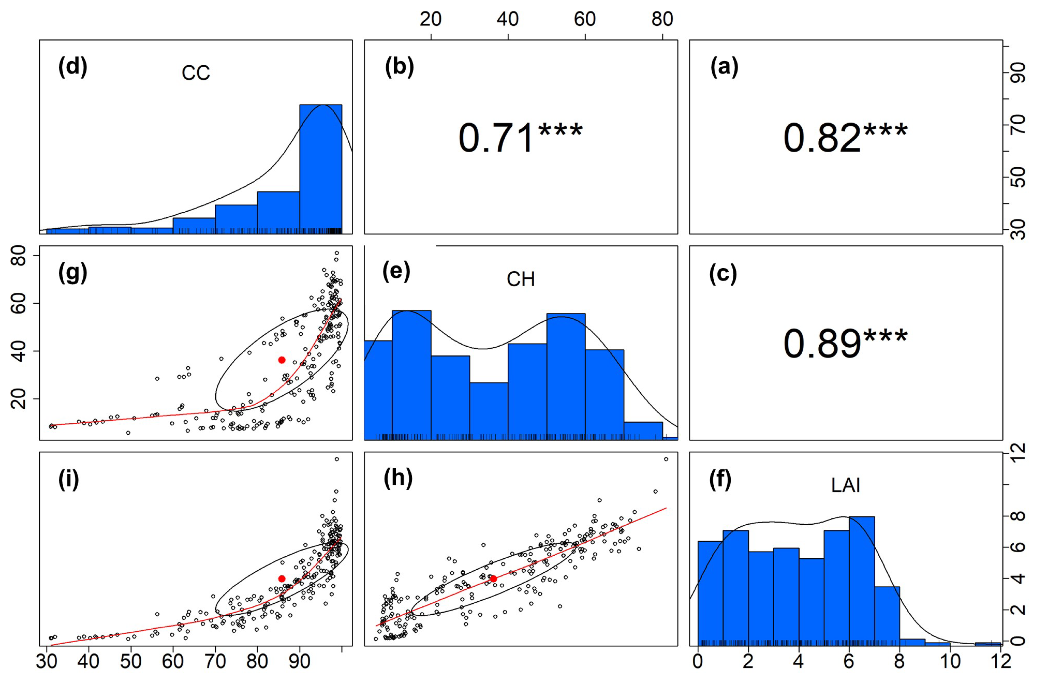
The Weibull distribution was the best fit for the CC data, with values of 8.08 and 91.53 for the shape and scale parameters, respectively (Figure 6d). In the histogram of CC, a higher frequency for CC values above 90% was observed than for smaller values. However, the scatterplot of CC and LAI showed an exponential trend with a correlation coefficient of 0.82 (Figure 6i). Similarly, the Weibull distribution was the best fit for the CH data, with values of 1.73 and 40.67 for the shape and scale parameters, respectively (Figure 6e). However, the density plot indicated that the data had a bimodal distribution and was depicted by the histogram in a similar way. The scatterplot of CH and LAI showed a linear trend with a correlation coefficient of 0.89 and a narrower correlation ellipse (Figure 6h). LAI data were also fitted to a Weibull distribution, with values of 1.62 and 4.38 for the shape and scale parameters (Figure 6f). The scatterplot of CC and CH showed a nonlinear trend, with a correlation coefficient of 0.71 and a wider correlation ellipse (Figure 6g).
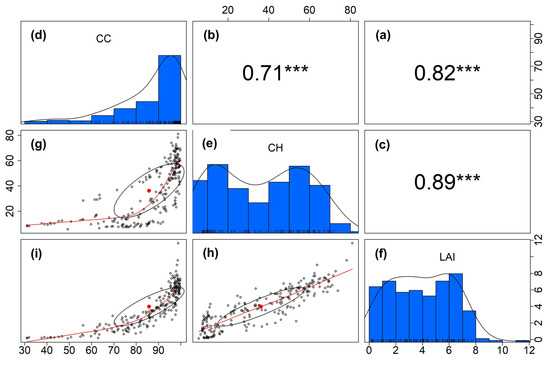
Figure 6.
Pearson’s correlation among canopy cover (CC), canopy height (CH), and leaf area index (LAI) (a–c); histograms of CC, CH, and LAI (d–f); and scatterplots relating CC, CH, and LAI (g–i) with ellipses around the mean (red dot) reflecting the correlation and the red line of best fit between the parameters. *** p < 0.001.
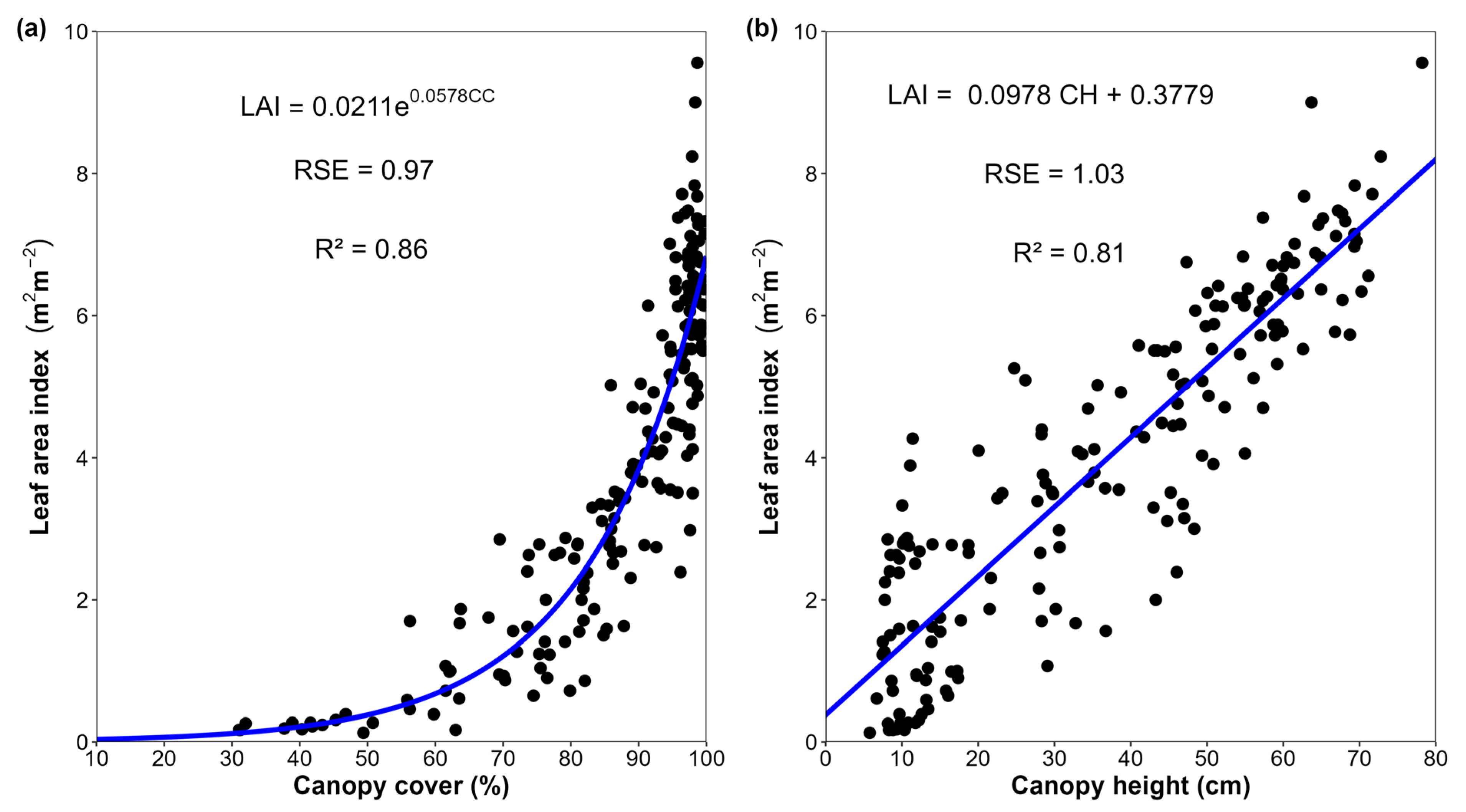
An exponential model of LAI as a function of CC was fitted to the training dataset, with a residual standard error (RSE) of 0.97 and R2 of 0.86 (Figure 7a). As indicated before, fewer data points with small CC values were used to fit the model, and more data points with values between 90% and 100%. With this model, it is possible to estimate the LAI using as input CC (Equation (3)).
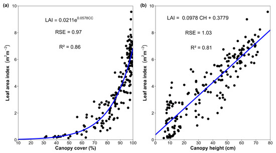
Figure 7.
Exponential model of leaf area index (LAI) as a function of canopy cover (CC) (a) and simple linear regression (SLR) model of LAI as a function of canopy height (CH) (b).
The SLR model of LAI as a function of CH was fitted with an RSE, R2, and p-value of 1.03, 0.81, and <2.2 × 10⁻¹⁶, respectively (Equation (4)). A higher spread of the data points was observed for small values of CH and LAI than for larger values (Figure 7b). Additionally, the MLR model of LAI as a function of CC and CH was fitted with an RSE, R2, and p-value of 0.82, 0.88, and <2.2 × 10⁻¹⁶, respectively (Equation (5)).
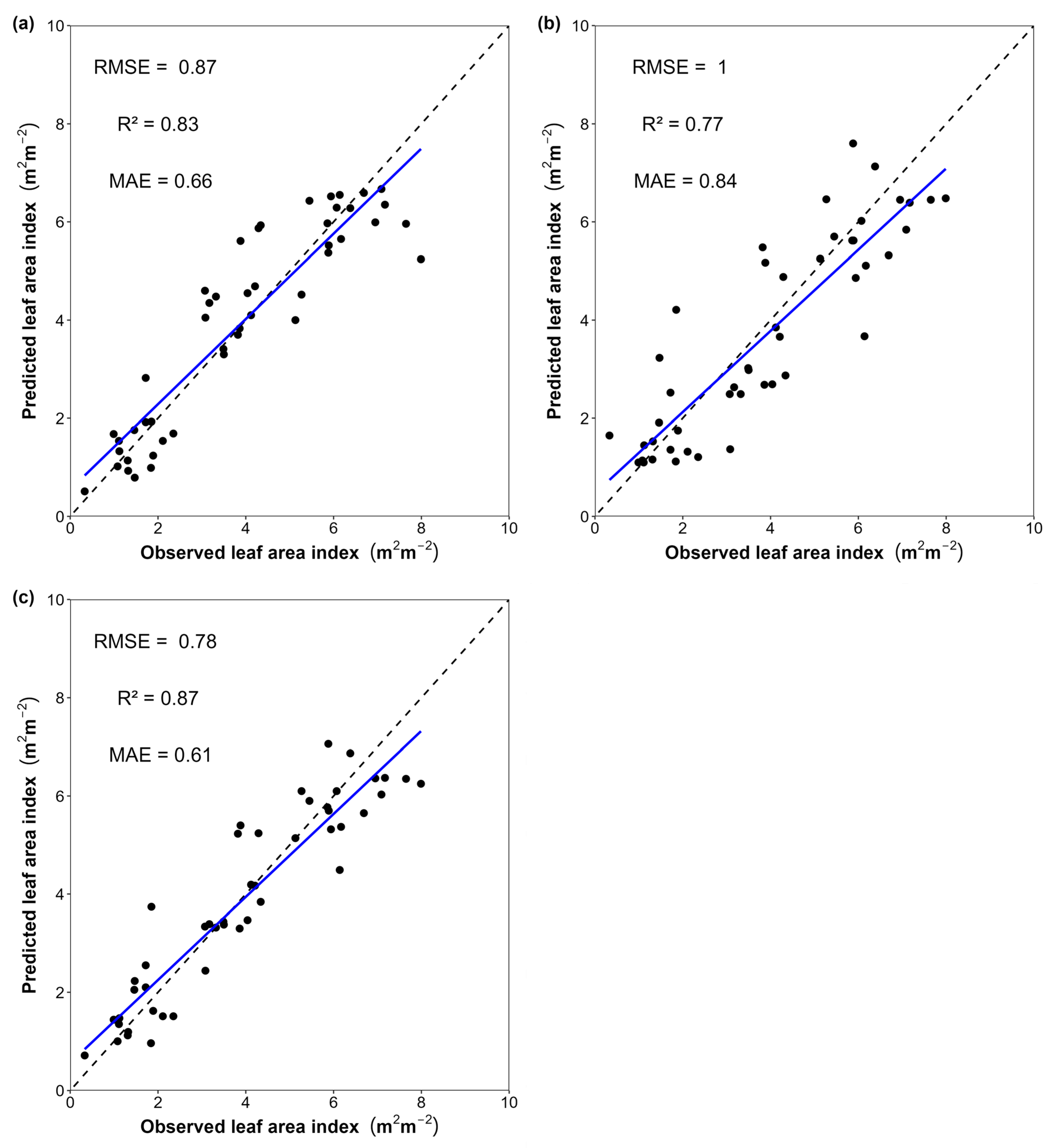
The validation of the exponential model of LAI as a function of CC resulted in an R2, RMSE, and MAE of 0.83, 0.87, and 0.66, respectively (Figure 8a). It can be observed that the line of best fit had a lower slope than the 1:1 line, overpredicting LAI values below four and simultaneously underpredicting higher LAI values.

Figure 8.
Relationship between the observed and predicted leaf area index (LAI) obtained using CC as the predictor of LAI (a), i.e., Equation (3), CH as the predictor of LAI (b), i.e., Equation (4), and CC and CH as predictors of LAI (c), i.e., Equation (5). The blue line represents the best fit for the plotted points, and the dashed black line represents where the points would be if the predicted values matched the observed values.
Similarly, the SLR model of LAI as a function of CH was validated with an R2, RMSE, and MAE of 0.77, 1, and 0.84, respectively (Figure 8b). The line of best fit exhibited a smaller slope than the 1:1 line; this model tends to overestimate small values while underestimating large LAI values.
The validation of the MLR model of LAI as a function of CC and CH had an R2, RMSE, and MAE of 0.87, 0.78, and 0.61, respectively (Figure 8c). The line of best fit also had a smaller slope compared to the 1:1 line, therefore, the model tends to overpredict small LAI values and underpredict large LAI values.
The results of the analysis of variance showed that the irrigation treatment, alfalfa variety, and the date of collection were not significant (p > 0.05) for the LAI, CC, and CH. Therefore, the summary tables of this analysis are not presented as part of the results.
4. Discussion
It was at the start of the 2022 season when low CC and LAI were measured. However, the lowest mean CC, LAI, and CH in both seasons were obtained eight days after the second harvest period during the 2021 season (Table 3). During the growing season of 2022, an earlier alfalfa regrowth was observed due to the moisture contribution of snowfall during the last months of winter. Moreover, fully developed crowns and deeper roots in the 2022 season may have allowed alfalfa to access water stored deeper in the soil profile. On the other hand, obtaining the highest LAI and CH before the first harvest period in both seasons (Table 3) could be attributed to the water availability, optimum temperatures, and solar radiation that contributed to stem elongation and leaf expansion. High LAI values contribute to increasing sunlight interception and CO2 assimilation by the canopy when the environmental conditions are suitable [31]. However, Liu et al. [3] observed, for alfalfa under deficit irrigation, a reduction in forage accumulation, LAI, plant relative water content, and radiation use efficiency. In addition, a longer period between the start of the growing season and the date of the first cut could have contributed to higher LAI values before the first harvest period when compared to the remaining periods, in which the alfalfa was harvested with intervals between cuts of approximately 28 days.
A higher variability of CC and CH in the season 2021 may have occurred due to a less developed root system that contributed to intensifying the effects of water stress for the mild and moderate deficit irrigation treatments. Therefore, water stress affected the growth and development of alfalfa subjected to these treatments and increased the gap with respect to the full irrigation treatment. These results agree with the findings of Brown and Tanner [32], who described that water stress in alfalfa decreased both the growth rate and relative growth rate. Similarly, Mouradi et al. [33] found major reductions in alfalfa dry biomass and CH due to water stress. Although CH and CC followed the same trend as LAI throughout the two growing seasons, the trend of CH data was closer to the trend exhibited by the LAI data. This is supported by the higher correlation of LAI with CH than with CC (Figure 6c). However, the scatterplot of CC and LAI (Figure 6i) showed that the relationship between them was exponential instead of linear, and it was not detected by the correlation.
The higher frequency of CC values between 90% and 100% was due mainly to the developmental stages in which the data collection occurred (Figure 6d). One of the limitations of this study is that most of the data were collected at the early bud and early flower stages, with limited data collected at the early vegetative and mid-vegetative stages. Nevertheless, the data used to find the relationship between the CC, CH, and LAI included a wide range of values (Figure 5) because they were obtained from two alfalfa varieties subjected to different irrigation treatments (Figure 1). Even though the best fit for the CH data was a Weibull distribution, the empirical probability density function indicated that the CH data had a bimodal distribution. This is mainly due to the combination of plots that were fully irrigated and plots subjected to deficit irrigation. Thus, there were two means, one corresponding to the mild and moderate deficit irrigation treatment and the other to the full irrigation treatment. The higher frequency of LAI values between six and seven (Figure 6f) is explained by the recurrent data collection before each harvest when LAI values were higher than at earlier developmental stages.
It has been reported that deficit irrigation in alfalfa reduces LAI due to water stress [3,34]. Under water stress, the leaf expansion rate is reduced and results in a reduction of the transpiration to prevent leaf tissue dehydration [35]. Regarding CC, Hanson et al. [36] found statistically significant differences in CC and CH between deficit irrigated treatments and full irrigation (t-test, level of significance = 0.05) during the periods of deficit irrigation. However, although the LAI, CC, and CH values in the plots under mild and moderate deficit irrigation in this study were lower than in the plots under full irrigation, the irrigation treatment was not a significant factor for the response variables in both growing seasons. Similar results were found during the 2022 season, when irrigation treatment had no significant effect on the alfalfa dry yield. However, during the 2021 season, the irrigation treatment (p < 0.05) had a significant effect on the alfalfa dry yield [37]. It should be noted that approximately seventy percent of the data used for this study was collected in 2022.
A good fit was obtained with a residual standard error (RSE) of 0.97 on 183 degrees of freedom after fitting the exponential model to the training dataset. Córcoles et al. [22] obtained an RSE of 19.72 for an exponential model of LAI in onion using CC as its predictor. When the model was assessed with the testing dataset, the RMSE and the MAE were small. Xiong et al. [11] found similar results fitting an exponential model to Old World bluestem clover data, with RMSE values ranging from 0.33 to 1.34. Even though the technique utilized to collect the CC data for this study is considered proximal sensing, it still has the same limitations as remote sensing methods. Raj et al. [38] indicated that estimation of LAI using remote sensing techniques shows good performance for early growth stages, but during the reproductive stage, they are prone to generate high error due to canopy closure. For this study, higher errors in the prediction of LAI were observed at the early flowering stage.
The SLR model of LAI as a function of CH was fitted with a slightly higher RSE (1.03) than the exponential model of LAI as a function of CC. For the validation of the linear model, the RMSE and MAE were also higher than those obtained with the exponential model. Labbafi et al. [24] reported RMSE values between 4.79 and 5.13 for a linear model to estimate the LAI of Cucurbita pepo L. with CH as the predictor for three planting dates. The MLR model of LAI as a function of CC and CH performed better than the exponential and SLR models for both training and testing (RMSE = 0.78, MAE = 0.61). Hammond et al. [26] obtained comparable results for an MLR using visible vegetation indices and CH as the predictors, with an RMSE between 0.67 and 1.01. Similarly, Raj et al. [38] found an RMSE ranging from 0.36 to 0.45 for an MLR model to estimate the LAI of maize using CC, CH, and a vertical leaf area distribution factor.
The models presented in this study can be used by crop modelers or farmers to estimate alfalfa LAI when CC, CH, or both predictors are available. When both predictors are available, the accuracy in the estimation of LAI can improve with the MLR model. However, if only one of these predictors can be measured due to time constraints, it is recommended to collect CC since the exponential model using this predictor was the second-best model. Furthermore, there have been some studies that mounted infrared thermometers to the frames of center pivot irrigation systems to automate the site-specific collection of canopy temperatures in fields irrigated with these systems [39,40]. Similarly, an RGB camera and/or an ultrasonic sensor can be mounted to the frame of center pivot or linear move irrigation systems to facilitate the site-specific collection of alfalfa CC and CH data. The models introduced in this study can be used under such scenario to estimate site-specific alfalfa LAI data that can be fed to crop growth models to improve their outcomes.
5. Conclusions
A nonlinear relationship was found between CC and LAI values. The exponential model for the prediction of LAI as a function of CC was a good fit (RSE = 0.97, R2 = 0.86) for the training dataset. With the testing dataset, the model performed well, with an RMSE of 0.87, R2 of 0.83, and MAE of 0.66. The SLR model of LAI with CH as the predictor for the training dataset had a lower performance than the exponential model (RSE = 1.03, R2 = 0.82). In validation, the SLR regression model showed a similar pattern, with an RMSE of 1, coefficient of determination of 0.77, and MAE of 0.88. An MLR model with CC and CH as the predictors improved the estimation of LAI (RSE = 0.82, R2 = 0.88). The validation of the MLR model also produced the best results, with an RMSE of 0.78, R2 of 0.87, and MAE of 0.66. These three models can be used to estimate LAI when CC, CH, or both predictors are available. The LAI values estimated with these models could serve as inputs for crop growth models when LAI measurements are not available.
Author Contributions
Conceptualization, U.C. and M.A.A.; methodology, U.C. and M.A.A.; software, U.C.; validation, U.C.; formal analysis, U.C.; investigation, U.C.; resources, M.A.A. and J.K.Q.S.; data curation, U.C.; writing—original draft preparation, U.C.; writing—review and editing, U.C., M.A.A. and J.K.Q.S.; supervision, U.C., M.A.A. and J.K.Q.S.; project administration, M.A.A.; funding acquisition, M.A.A. All authors have read and agreed to the published version of the manuscript.
Funding
This research was supported by the University of Nevada, Reno, Office of Research and Innovation, the Nevada Agricultural Experiment Station of the College of Agriculture, Biotechnology & Natural Resources, University of Nevada, Reno, and the Engineering for Precision Crop and Water Management program, project award no. 2023-67022-40558, from the U.S. Department of Agriculture’s National Institute of Food and Agriculture.
Data Availability Statement
The data presented in this study are available on request from the corresponding author.
Acknowledgments
The authors acknowledge the dedicated work performed by Scott Huber, Senior Assistant Director of the Nevada Agricultural Experiment Station.
Conflicts of Interest
The authors declare no conflicts of interest.
References
- Chen, J.M.; Black, T.A. Defining Leaf Area Index for Non-Flat Leaves. Plant Cell Environ. 1992, 15, 421–429. [Google Scholar] [CrossRef]
- Dobrenz, A.K.; Back, M. Changing the Leaf Area on Alfalfa; Forage and Grain: A college of Agriculture Report; College of Agriculture, University of Arizona: Tucson, AZ, USA, 1984; pp. 6–7. Available online: https://repository.arizona.edu/handle/10150/200452 (accessed on 1 October 2021).
- Liu, M.; Mu, L.; Lu, Y.; Yang, H. Forage Accumulation and Radiation Use of Alfalfa under Deficit Irrigation. Crop Sci. 2021, 61, 2190–2202. [Google Scholar] [CrossRef]
- Nelson, C.J.; Smith, D. Growth of Birdsfoot and Alfalfa. III Changes in Carbohydrates Reserves and Growth Analysis Under Field Conditions1. Crop Sci. 1968, 8, 25–28. [Google Scholar] [CrossRef]
- Bolger, T.P.; Matches, A.G. Water-Use Efficiency and Yield of Sainfoin and Alfalfa. Crop Sci. 1990, 30, 143–148. [Google Scholar] [CrossRef]
- Greub, L.J.; Wedin, W.F. Leaf Area, Dry-Matter Accumulation, and Carbohydrate Reserves of Alfalfa and Birdsfoot Trefoil Under a Three-Cut Management1. Crop Sci. 1971, 11, 341–344. [Google Scholar] [CrossRef]
- Afsharmanesh, G. Study of Some Morphological Traits and Selection of Drought-Resistant Alfalfa Cultivars (Medicago sativa L.) in Jiroft, Iran. Plant Ecophysiol. 2009, 3, 109–118. [Google Scholar]
- Rimi, F.; Macolino, S.; Leinauer, B.; Lauriault, L.M.; Ziliotto, U. Alfalfa Yield and Morphology of Three Fall-Dormancy Categories Harvested at Two Phenological Stages in a Subtropical Climate. Agron. J. 2010, 102, 1578–1585. [Google Scholar] [CrossRef]
- Patrignani, A.; Ochsner, T.E. Canopeo: A Powerful New Tool for Measuring Fractional Green Canopy Cover. Agron. J. 2015, 107, 2312–2320. [Google Scholar] [CrossRef]
- Trout, T.J.; Johnson, L.F.; Gartung, J. Remote Sensing of Canopy Cover in Horticultural Crops. HortScience 2008, 43, 333–337. [Google Scholar] [CrossRef]
- Xiong, Y.; West, C.P.; Brown, C.P.; Green, P.E. Digital Image Analysis of Old World Bluestem Cover to Estimate Canopy Development. Agron. J. 2019, 111, 1247–1253. [Google Scholar] [CrossRef]
- Baxter, L.L.; West, C.P.; Brown, C.P.; Green, P.E. Comparing Nondestructive Sampling Techniques for Predicting Forage Mass in Alfalfa–Tall Wheatgrass Pasture. Agron. J. 2017, 109, 2097–2106. [Google Scholar] [CrossRef]
- Jones, J.W.; Hoogenboom, G.; Porter, C.H.; Boote, K.J.; Batchelor, W.D.; Hunt, L.A.; Wilkens, P.W.; Singh, U.; Gijsman, A.J.; Ritchie, J.T. The DSSAT Cropping System Model. Eur. J. Agron. 2003, 18, 235–265. [Google Scholar] [CrossRef]
- Keating, B.A.; Carberry, P.S.; Hammer, G.L.; Probert, M.E.; Robertson, M.J.; Holzworth, D.; Huth, N.I.; Hargreaves, J.N.G.; Meinke, H.; Hochman, Z.; et al. An Overview of APSIM, a Model Designed for Farming Systems Simulation. Eur. J. Agron. 2003, 18, 267–288. [Google Scholar] [CrossRef]
- Geerts, S.; Raes, D.; Garcia, M. Using AquaCrop to Derive Deficit Irrigation Schedules. Agric. Water Manag. 2010, 98, 213–216. [Google Scholar] [CrossRef]
- Holman, J.; Min, D.; Klocke, N.; Kisekka, I.; Currie, R. Effects of Irrigation Amount and Timing on Alfalfa Nutritive Value. Trans. ASABE 2016, 59, 849–860. [Google Scholar] [CrossRef]
- Linker, R.; Kisekka, I. Model-Based Deficit Irrigation of Maize in Kansas. Trans. ASABE 2017, 60, 2011–2022. [Google Scholar] [CrossRef]
- Linker, R.; Ioslovich, I.; Sylaios, G.; Plauborg, F.; Battilani, A. Optimal Model-Based Deficit Irrigation Scheduling Using AquaCrop: A Simulation Study with Cotton, Potato and Tomato. Agric. Water Manag. 2016, 163, 236–243. [Google Scholar] [CrossRef]
- Thorp, K.; Hunsaker, D.; Bronson, K.; Andrade-Sanchez, P.; Barnes, E. Cotton Irrigation Scheduling Using a Crop Growth Model and FAO-56 Methods Field and Simulation Studies. Trans. ASABE 2017, 60, 2023–2039. [Google Scholar] [CrossRef]
- Linker, R.; Kisekka, I. Concurrent Data Assimilation and Model-Based Optimization of Irrigation Scheduling. Agric. Water Manag. 2022, 274, 107924. [Google Scholar] [CrossRef]
- Nielsen, D.C.; Miceli-Garcia, J.J.; Lyon, D.J. Canopy Cover and Leaf Area Index Relationships for Wheat, Triticale, and Corn. Agron. J. 2012, 104, 1569–1573. [Google Scholar] [CrossRef]
- Córcoles, J.I.; Ortega, J.F.; Hernández, D.; Moreno, M.A. Estimation of Leaf Area Index in Onion (Allium cepa L.) Using an Unmanned Aerial Vehicle. Biosyst. Eng. 2013, 115, 31–42. [Google Scholar] [CrossRef]
- Liu, J.; Pattey, E. Retrieval of Leaf Area Index from Top-of-Canopy Digital Photography over Agricultural Crops. Agric. For. Meteorol. 2010, 150, 1485–1490. [Google Scholar] [CrossRef]
- Labbafi, M.; Khalaj, H.; Allahdadi, I.; Nadjafi, F.; Akbari, G.A. Using Models for Estimation of Leaf Area Index in Cucurbita pepo L. J. Saudi Soc. Agric. Sci. 2019, 18, 55–60. [Google Scholar] [CrossRef]
- Logsdon, S.D.; Cambardella, C.A. An Approach for Indirect Determination of Leaf Area Index. Trans. ASABE 2019, 62, 655–659. [Google Scholar] [CrossRef]
- Hammond, K.; Kerry, R.; Jensen, R.R.; Spackman, R.; Hulet, A.; Hopkins, B.G.; Yost, M.A.; Hopkins, A.P.; Hansen, N.C. Assessing Within-Field Variation in Alfalfa Leaf Area Index Using UAV Visible Vegetation Indices. Agronomy 2023, 13, 1289. [Google Scholar] [CrossRef]
- WRCC. Station Daily Time Series. Available online: https://wrcc.dri.edu/cgi-bin/rawMAIN2.pl?nvunrc (accessed on 1 October 2021).
- Soil Survey Staff; NRCS; USDA. Web Soil Survey. Available online: https://websoilsurvey.sc.egov.usda.gov/App/HomePage.htm (accessed on 15 March 2022).
- R Core Team. The R Project for Statistical Computing. Available online: https://www.r-project.org/ (accessed on 3 December 2021).
- Tuszynski, J. CaTools: Tools: Moving Window Statistics, GIF, Base64, ROC, AUC, Etc. 2021. R package version 1.18.2. Available online: https://CRAN.R-project.org/package=caTools (accessed on 1 October 2021).
- Hanson, A.A.; Barnes, D.K.; Hill, R.J. Alfalfa and Alfalfa Improvement; American Society of Agronomy, Crop Science Society of America, Soil Science Society of America: Madison, WI, USA, 1988. [Google Scholar]
- Brown, P.W.; Tanner, C.B. Alfalfa Stem and Leaf Growth During Water Stress. Agron. J. 1983, 75, 799–805. [Google Scholar] [CrossRef]
- Mouradi, M.; Bouizgaren, A.; Farissi, M.; Ghoulam, C. Assessment of Deficit Irrigation Responses of Moroccan Alfalfa (Medicago sativa L.) Landraces Grown Under Field Conditions. Irrig. Drain. Irrig. Drain 2018, 67, 179–190. [Google Scholar] [CrossRef]
- Saeed, I.A.M.; El-Nadi, A.H. Irrigation Effects on Growth, Yield, and Water Use Efficiency of Alfalfa. Irrig. Sci. 1997, 17, 63–68. [Google Scholar] [CrossRef]
- Liu, F.; Stützel, H. Leaf Expansion, Stomatal Conductance, and Transpiration of Vegetable Amaranth (Amaranthus sp.) in Response to Soil Drying. J. Am. Soc. Hortic. Sci. 2002, 127, 878–883. [Google Scholar] [CrossRef]
- Hanson, B.; Putnam, D.; Snyder, R. Deficit Irrigation of Alfalfa as a Strategy for Providing Water for Water-Short Areas. Agric. Water Manag. 2007, 93, 73–80. [Google Scholar] [CrossRef]
- Cholula, U.; Quintero, D.; Andrade, M.A.; Solomon, J. Effects of Deficit Irrigation on Yield and Water Productivity of Alfalfa in Northern Nevada. In 2022 ASABE Annual International Meeting; American Society of Agricultural and Biological Engineers: Houston, TX, USA, 2022. [Google Scholar]
- Raj, R.; Walker, J.P.; Pingale, R.; Nandan, R.; Naik, B.; Jagarlapudi, A. Leaf Area Index Estimation Using Top-of-Canopy Airborne RGB Images. Int. J. Appl. Earth Obs. Geoinf. 2021, 96, 102282. [Google Scholar] [CrossRef]
- Peters, R.T.; Evett, S.R. Spatial and Temporal Analysis of Crop Conditions Using Multiple Canopy Temperature Maps Created with Center-Pivot-Mounted Infrared Thermometers. Trans. ASABE 2007, 50, 919–927. [Google Scholar] [CrossRef]
- O’Shaughnessy, S.A.; Andrade, M.A.; Evett, S.R. Using an Integrated Crop Water Stress Index for Irrigation Scheduling of Two Corn Hybrids in a Semi-Arid Region. Irrig. Sci. 2017, 35, 451–467. [Google Scholar] [CrossRef]


Disclaimer/Publisher’s Note: The statements, opinions and data contained in all publications are solely those of the individual author(s) and contributor(s) and not of MDPI and/or the editor(s). MDPI and/or the editor(s) disclaim responsibility for any injury to people or property resulting from any ideas, methods, instructions or products referred to in the content. |
© 2024 by the authors. Licensee MDPI, Basel, Switzerland. This article is an open access article distributed under the terms and conditions of the Creative Commons Attribution (CC BY) license (https://creativecommons.org/licenses/by/4.0/).