Abstract
Coffee production has become increasingly technified in order to optimize the use of inputs and the sustainable use of natural resources. In this context, one way that farmers are investing in their coffee plantations is in the use of precision agriculture techniques, termed precision coffee farming. Over the last few years, research has been conducted to facilitate the application of this technology, and sampling grids with two points per hectare have been recommended by several studies. These georeferenced demarcations in a plot are generally shaped as equidistant squares or rectangles, and the sampling points are located at the centers of these areas. Coffee farmers typically plant their crops following the level line, which greatly hinders the navigation of equidistant points within the field. Thus, the objective of this study was to develop an optimized walking route method to reduce the distance for sampling soil, leaf, and yield attributes. The experimental plots were established in 2000 at Samambaia Farm, located in Santo Antônio do Amparo, Minas Gerais, Brazil, with coffee the cultivar Acaia IAC 479-19, totaling 56.65 ha. The 111 sampling points were distributed in the land following the new method proposed in this study, and, after walking simulations using Farm Works Mapping Software, the new method was compared with the conventional method using the mean displacement between points. The new optimized walking routes method reduced the mean distance traveled to sample the points by 50.1%.
1. Introduction
The technological advances applied to agriculture are responsible for productivity and efficiency gains in production units. The advent of modernized agriculture has led to improvements in production and better adaptation of production to market requirements, increasing the competitiveness of producers [1]. Localized crop management aims to optimize agricultural production by managing crops and soil according to the different conditions found in each field [2]. This localized management is called precision agriculture, and, in order to perform it, detailed information on the heterogeneity of crop fields is necessary to adjust soil cultivation, sowing, fertilization, and pesticide application to local conditions. In conventional agriculture, the existing information on soil and plants rarely corresponds to the requirements necessary for production [3]. Precision agriculture is based on the spatial variability of the cultivation area, in contrast to conventional agriculture, which works with field means, thus reducing input application losses and environmental damage [4].
Precision coffee farming is a concept that implies the use of precision agriculture techniques in coffee plantations [5]. Understanding the spatial variability in a field requires a greater amount of data obtained from samplings of representative grids [6,7]. In addition to georeferenced soil analyses and variable-rate fertilizer applications, yield maps are of great importance for precision coffee farming cycles, in particular, to compare the applied products with the local yield of coffee plants and to determine the production patterns of a field [5,6,8,9,10,11,12]. The studies conducted by [13,14,15,16] found that the application of the two-points-per-hectare method was the most recommended as it makes it possible to observe the spatial variability in some soil and leaf chemical attributes and the yield of coffee plants. In geostatistics, the most commonly used sampling grid is a systematic grid, where the evaluated points are distributed in a two-dimensional, equidistant (square or rectangular) shape. Although equidistance between the points is not mandatory, it is necessary to georeference the data to perform spatial analyses. Ref. [17] conducted a survey of the type of sampling grid, area size, and number of points used in geostatistical studies published on the SciELO database between 1997 and 2010 and found that 82.54% of the published articles used regular grids while 17.46% used irregular soil sampling grids. Additionally, the most commonly used grid sampling strategy is point sampling, i.e., where samples are collected at the central point of the grid [16,18,19].
Currently, when coffee is planted in sloping areas, it is still typical for the furrowing of the land to follow an alignment made by base leveling; in terrain with favorable topography, allocation and furrowing can performed in straight and parallel lines [20,21]. However, in both cases, the equidistant allocation of sampling points hinders the movement of the individual carrying out the sampling inside the field. The objective of this study was to develop a sampling method through the optimization of walking routes in coffee fields to reduce the time spent in and the displacement required for the operation.
2. Materials and Methods
The present study was conducted at Samambaia Farm, located in the municipality of Santo Antônio do Amparo, Southern Minas Gerais state, Brazil, at mean geographic coordinates of 20°58′19.92″ S and 44°53′24.18″ W. The experimental site has 56.65 hectares of Coffea arabica L. coffee plants of the Acaiá IAC 474-19 cultivar, planted in the year 2000, with spacing of 3.6 m between rows and 0.8 m between plants. The area is divided into four plots named ZE02 (5.9 ha), ZE03 (30.25 ha), ZE06 (8.5 ha), and ZE08 (10.0 ha). The soil is classified as dystrophic red–yellow latosol with clayey texture and a gently undulating relief. In the 0.0–0.20 m layer, the average particle size fractions are as follows: 38% clay, 10% silt, 52% sand. The climate at the site is characterized as mild, highland tropical, with moderate temperatures and hot and rainy summers, with a Köppen classification of Cwa.
The field under study was demarcated in a regular sampling grid using an adapted method, with two points per hectare, as recommended for precision coffee farming and indicated in optimal grid index studies [13,15,16,22,23,24].
2.1. Proposed Method
Considering that most coffee plantations in southern Minas Gerais have leveled planting rows, a method based on the equidistant square sampling grid that aims to reduce walking within the plot using “walking routes” was developed. Figure 1 illustrates an easy-to-navigate walking route with points aligned along the same path, eliminating the need for the sampler to cross planting rows.
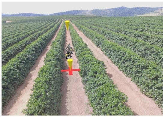
Figure 1.
Example of an easy walking route with sampling points indicated by X marks and yellow arrows.
The standard procedure for generating sampling grids by geographic information systems (GISs) typically yields perfectly square grids, whose inflexibility may pose challenges in the practical implementation of the sampling method. As illustrated in Figure 2, the one-point-per-hectare sampling grid (Figure 2A) is represented by a 100 × 100-m2, whereas the equidistant square for the two-point-per-hectare sampling grid measures 70.71 m × 70.71 m (Figure 2B).
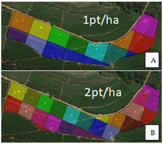
Figure 2.
Example of automatic creation of sampling grids generated by a GIS like Trimble’s Farm-Works 2014.09.36: one point per hectare (A); two points per hectare (B). Each colored square represents a sampling grid, with the colored central points indicating the sampling locations.
The development of this method necessitates current satellite images, such as those from Google Earth PRO 7.3.6.9796 (64-bit), along with high plot resolution to enable a clear differentiation of planting rows, inter-rows, towpaths, faults, and other relevant features. The distribution of points within the plot significantly impacts the results of point interpolation. Therefore, selecting a plot side that aligns with the planting rows is of paramount importance.
As described earlier, the sampling methodology employed adheres to precision coffee farming studies, which advocate for two sampling points per hectare. Consequently, the sampling points are spaced approximately 70.71 m apart, rounded to 70 m. As depicted in Figure 1, the walking routes should align with the coffee rows to optimize the sampler’s movement.
To delineate the initial walking route, the side of the terrain parallel to the coffee rows is considered. From the midpoint of the plot’s length, a distance of 35 m is measured from the plot edge, establishing the first walking route, as illustrated in Figure 3. Subsequent routes are then traced at regular intervals of 70 m. It is noteworthy that, in certain fields, variations in inter-row distances and the width of parallel pathways may impact the placement of these routes.
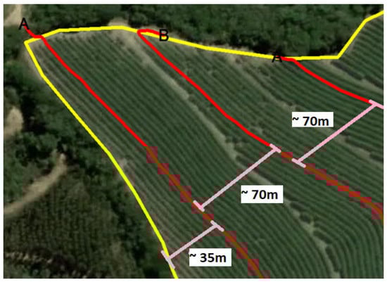
Figure 3.
Plot ZE08 after defining the initial walking routes with two points per hectare. The red lines are the walking routes, the yellow line is the plot boundary, and points A and B indicate the start and end of the walking routes, respectively.
Once the navigation lines have been drawn across the plot (Figure 4), the next step is to draw auxiliary lines to mark sampling points. These lines should start parallel to the opposite side of the field, which is perpendicular to the navigation lines. The first auxiliary line should be at least 35 m away from the edge of the field and ideally intersect the navigation lines at a 90° angle, as shown in Figure 5.
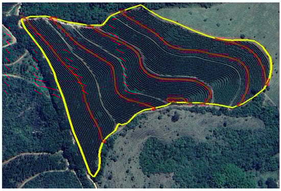
Figure 4.
Plot ZE08 after delineating the walking routes using the method described above. The red lines are the walking routes, the yellow line is the plot boundary.
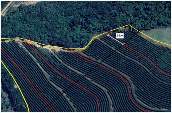
Figure 5.
Main auxiliary line drawn in plot ZE08. The red lines are the walking routes following the coffee plant rows, and the black line crossing the walking routes is the auxiliary line. The yellow line is the plot boundary.
After establishing the main auxiliary line, parallel auxiliary lines, known as offsets, need to be created at intervals of 70 m. The quantity of auxiliary lines required varies depending on the plot layout. In the case of plot ZE08, six lines were drawn: two to the left and four to the right of the main auxiliary line, ensuring comprehensive coverage of the entire terrain (Figure 6).
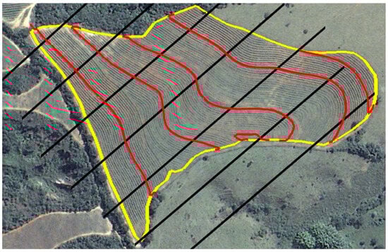
Figure 6.
Parallel auxiliary lines were drawn in plot ZE08, with four to the right and six to the left of the main auxiliary line. The red lines are the walking routes following the coffee plant rows, and the black lines crossing the walking routes are the auxiliary lines. The yellow line is the plot boundary.
The sampling points are allocated at the intersections of the walking routes with the auxiliary lines. It is crucial to assign numbers to the sampling points in the order corresponding to the sequence in which the routes will be traversed during field sampling, thereby mitigating potential issues (Figure 7).
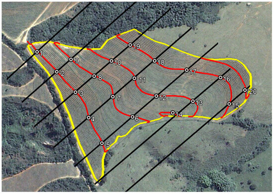
Figure 7.
The allocation of sampling points in plot ZE08 follows a predetermined sequence. Points 1 to 20 mark the sampling locations along the walking route. The red lines are the walking routes following the coffee plant rows, and the black lines crossing the walking routes are the auxiliary lines. The yellow line is the plot boundary.
In certain instances, sampling points may be situated in locations within the plot that are not representative, such as in towpaths or areas with faults. In such cases, it becomes necessary to relocate the point to a more representative position along the walking route. For instance, point 14 in Figure 7 was relocated within the field to ensure its representativeness.
After assigning the sampling points in the field, the auxiliary lines, which were used for guidance during the allocation process, can be removed. This leaves only the navigation lines intact. These navigation lines serve as guides during fieldwork, aiding in the proper entry into the inter-row spaces for sampling purposes, as demonstrated in Figure 8.
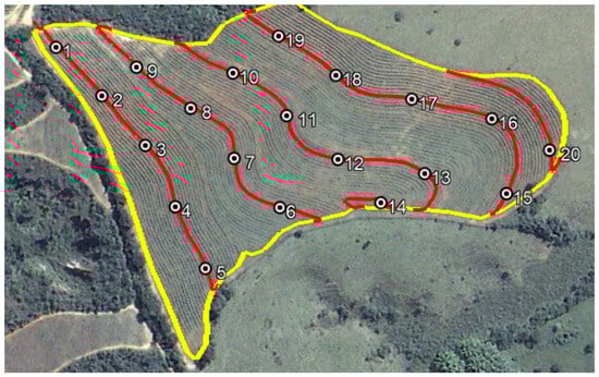
Figure 8.
Plot ZE08 displaying the walking routes delineated by red lines and the sampling points 1 to 20 allocated in the field. The yellow line is the plot boundary.
2.2. Methodological Flowchart for Walking Route and Sampling Point Creation
To systematically visualize the algorithmic approach for creating walking routes and sampling points in the field using the proposed methodology, the following flowchart (Figure 9) was developed. The primary outcome of this flowchart is the structured delineation of walking routes and the precise allocation of sampling points within a coffee plot. By adhering to this systematic methodology, the sampling process is optimized in terms of both efficiency and representativeness.
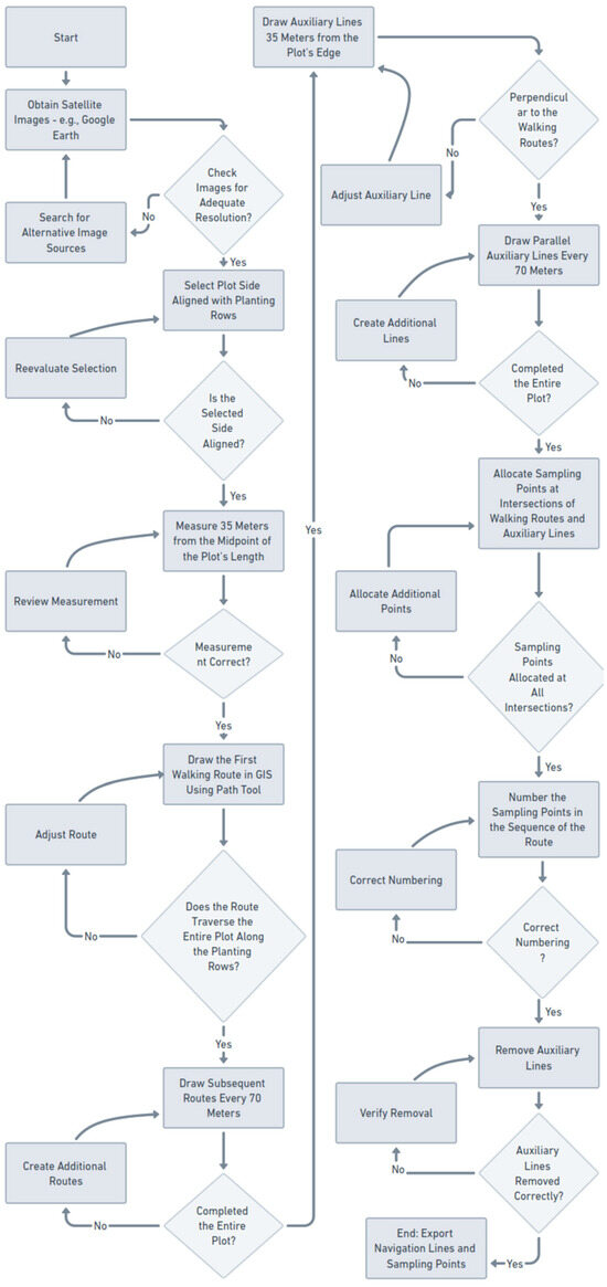
Figure 9.
Visualization of the methodological flowchart for creating walking routes and sampling points.
2.3. Sampling Grid Demarcation
The field under investigation was delineated using licensed Farm Works Office Version 2013.09.557, United States of America, to establish a sampling grid employing the proposed two-points-per-hectare method, as recommended in previous studies on optimal grid indexing for precision coffee farming. This grid comprised a total of 111 georeferenced sampling points distributed across plots ZE02 (12 points), ZE03 (60 points), ZE06 (18 points), and ZE08 (20 points) (Figure 10A–D). The sampling strategy employed in the grid was point sampling, where samples are collected at the central point of each grid cell. At these designated points, soil and leaf samples were collected, and a survey of plant productivity was conducted.
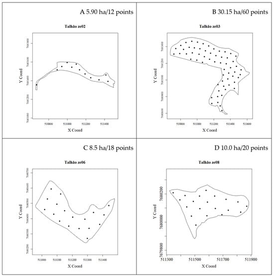
Figure 10.
Illustration of sketches of the sampling grids in the ZE02 (A), ZE03 (B), ZE06 (C), and ZE08 (D) plots. The Y coordinate represents latitude and the X coordinate represents longitude, both in meters.
For the creation of sampling points using the traditional method, the sampling grid generation tool in the Farm Works software was employed. The grid was configured to contain two points per hectare, distributed in a square and equidistant manner, with the resulting points resembling those depicted in Figure 2.
To facilitate a comparative analysis between the two methods, two distinct distances were calculated for each plot, each designed to cover an equivalent number of sampling points. One distance corresponded to the conventional method while the other reflected the proposed method. However, due to variations in plot sizes, a direct co24mparison between the methods proved impractical. To address this challenge, an index was formulated by dividing the distance traveled using each method by the number of sampling points within the respective plot. This approach yielded the mean distance traveled for sampling each individual point, thereby facilitating a more scientifically rigorous comparison between the two methodologies.
3. Results and Discussion
Various tools are accessible for data collection, storage, and analysis, facilitating studies on spatial variability. In numerous commercial coffee plantations earmarked for precision coffee farming, plots exhibit irregular shapes and are commonly established following the contour of the land.
Partitioning areas into square or rectangular sections of uniform and smaller dimensions represents a method for establishing standardized sampling grids [25]. However, the challenge is compounded in fields installed flush with the terrain contour, further complicating the sampling process.
Most farmers in coffee plantations commonly employ soil sampling quadrats. However, for samplers using vehicles to traverse between sampling points, extensive distances often need to be covered. This is primarily due to the fact that the sampling points are typically not aligned in a straight line, as depicted in Figure 11. Additionally, it is necessary to travel to the end of each inter-row to ascertain the correct entry point for sampling.
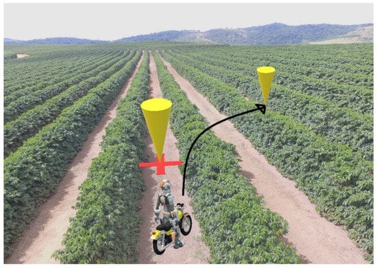
Figure 11.
Illustration of the challenge posed by navigating a regular sampling grid in coffee plantations, where coffee plants are spaced with inter-rows approximately 0.5 m apart. Yellow arrow with red X: current sampling point. Black arrow: path to the next sampling point (yellow arrow without X).
It is crucial to emphasize that searching for points within a coffee plantation or any other row-planted crop is extremely challenging. This is because, when planting on contour lines, the desired inter-row for sampling is not always accessible to the sampler, leading to time wasted in returning to the edge of the plot to restart the search process. This prolonged search for the sampling point significantly reduces work efficiency.
A study was conducted utilizing the geographic information system (GIS) functionalities within the Farm Works software to quantify the total distance traversed by the sampler to reach all sampling points. This study involved simulating the sampler’s paths within the plot to locate the sampling points, meticulously recording the distances traveled between consecutive points in meters. The sampler navigates to the closest sampling point within the same row, depending on the grid layout, and then proceeds to the next point in the most efficient direction, considering the terrain’s topography and any obstacles. This method ensures that the sampler only enters the desired inter-row for sampling. However, to move to the next point, it is necessary to return to the plot’s edge, as depicted in Figure 12. In this figure, the sampler moves to sampling point 1, returns to the edge, proceeds to sampling point 2, returns to the edge, and continues this pattern.
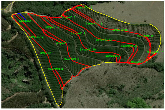
Figure 12.
Displays the simulated path (highlighted in red) taken by the sampler to reach the sampling points within an equidistant square grid, which is the primary method utilized in the agricultural field. The blue line represents the initial path leading to sampling point 1. The yellow line outlines the plot boundary.
This study employed a similar approach to evaluate the proposed methodology. Simulated paths were generated to represent the routes that a sampler would take to access the sampling points. Unlike the previous method, which required the sampler to repeatedly return to the field’s edge, in this approach, we calculated the distance traveled along the predefined walking route. This method aimed to assess the efficiency of the proposed walking route design in facilitating navigation between sampling points within the field.
In the demarcation of the walking routes in the field, variations in the distance between coffee rows were observed due to differences in planting distance, slope, and the width of towpaths. These variations underscore the necessity of accurately tracing the walking routes. Using GIS-based path simulations, where each route was manually traced in the software to simulate the sampling paths, the walking distances across all plots were quantified for both the conventional and proposed methods. This resulted in an analysis of means using the SISVAR software, Version: 5.6 Build: 90, UFLA Brazil, with 111 recorded values representing the walking distances required to reach all sampling points.
The simulation of the conventional method indicated a mean displacement of 263.2 m between sampling points, assuming that the individual conducting the sampling is aware of the inter-rows to be traversed in advance. Conversely, the simulations of the proposed method demonstrated a mean displacement of 132.8 m between sampling points (Table 1). This represents a significant reduction in the mean distance traveled by 130.4 m, leading to a considerable decrease in both the sampling time and associated costs.

Table 1.
Mean distances traveled in each plot to reach the sampling points in the conventional and proposed methods.
Upon analyzing Table 1, using the values obtained from the sampler’s walking simulations and in conjunction with SISVAR software, Version: 5.6 Build: 90, UFLA Brazil, it is evident that the proposed methodology yielded significantly different results according to the F-test at a 5% probability level, with an average reduction in distance traveled between sampling points of 50.1%. This reduction in distance and time results in decreased field sampling costs, further facilitating the implementation of precision coffee farming technologies.
Additionally, one can explore the option of virtually recreating the recommended walking routes using navigation applications available on smartphones or devices equipped with a global navigation satellite system (GNSS). Examples of such applications include MAPinr 3.8.0.0 Xylem Technologies, which offers comprehensive mapping functionalities. Moreover, for navigation between sampling points, farmers can utilize the Android application C7 GPS Malha v1.1, developed by the Laboratory of Geomatics of the Federal University of Santa Maria. These applications are freely accessible and provide practical solutions for farmers seeking efficient navigation and data collection in the field.
One of the earliest techniques employed to assess spatial or temporal dependence among neighboring samples is spatial or temporal sample autocorrelation, which quantifies this dependence. Alternatively, the semivariogram can be utilized to evaluate the relationship between adjacent points, focusing solely on spatial dependence [26]. Typically, the semivariogram is employed to assess the extent of spatial dependence among samples within a study area and to establish parameters essential for value estimation at unsampled locations using kriging methods [27].
The variation in the distance between points with the proposed method is another factor that may affect the quality of semivariograms. However, one way to support the effectiveness of the proposed method is to evaluate the yield data collected by the farm for two years. For the studied attribute, the spherical model best fits the semivariogram.
According to [28], the range values of the semivariogram separate the structured field, which has spatial dependence on the variable, from the random field, in which the pairs no longer show dependence (sill); that is, it has considerable importance in determining the limit of the spatial dependence, which may also be indicative of the interval between the soil mapping units [29] or plant-related attributes [6].
The geostatistical analysis method made it possible to quantify the magnitude and structure of the spatial dependence of the yield. Table 2 shows the results of this analysis for coffee yield in plots ZE02, ZE03, ZE06, and ZE08 for 2017 and 2018.
Table 2.
Estimation of the parameters for the spherical model fitted using ordinary least squares for the yield variable. The parameters included are the nugget effect (C0) and the range (a) in meters, for different plots and years.
Through the analysis of the estimated parameters of the spherical model for the yield variable, the nugget effect (C0) and range (a) can be evaluated (Table 2).
For the ZE02 plot, the nugget effect values were 1.44 in 2017 and 44.58 in 2018. The ranges were 155.87 m and 224.85 m, respectively. This substantial increase in both the nugget effect and range suggests greater spatial variability and an increase in the extent of spatial correlation over time.
In the ZE03 plot, the nugget effect values were 8.08 in 2017 and 0 in 2018. The ranges were 209.30 m and 112.47 m, respectively. The nugget effect in 2018 being zero indicates minimal measurement error or very-small-scale variability, whereas the significant decrease in range from 2017 to 2018 suggests a reduced extent of spatial correlation.
For the ZE06 plot, the nugget effect values were 0.28 in 2017 and 0.22 in 2018. The ranges were 118.52 m and 125.79 m, respectively. Both the nugget effect and range remained relatively stable across the two years, indicating consistent spatial variability and correlation over time.
In the ZE08 plot, the nugget effect values were 0 in 2017 and 36.86 in 2018. The ranges were 167.68 m and 78.95 m, respectively. The increase in the nugget effect from 0 to 36.86 and the decrease in the range from 167.68 m to 78.95 m indicate increased small-scale variability and a decreased extent of spatial correlation in 2018 compared to 2017.
The range values observed in Table 2 align with those reported in several studies. For instance, in the study by [9], conducted in a 22 ha area with 2.09 points per hectare, the coffee yield attribute reached a range of 165.34 m. Similar results were found by [22], who examined the optimal sampling density of coffee yield in precision coffee farming in a 26 ha area with a two-point per hectare grid, finding a range between 139.0 m and 236.1 m. Furthermore, ref. [23], also working with two points per hectare and coffee yield, found a range between 217.45 m and 963.21 m. These comparisons indicate that the range values obtained in the current study are consistent with those reported in the literature, reinforcing the validity of the spatial correlation results observed in the yield variable across different plots and years.
Table 2 reveals that the most restricted spatial correlation, as indicated by the lowest range, occurred in the ZE08 plot in 2018, measuring at 78.95 m. Remarkably, this range surpasses the findings of [30], who reported a range of 45.00 m for a grid with 50 points per hectare. Additionally, ref. [31] investigated Conilon coffee yield in Espírito Santo, Brazil, using cokriging techniques and a spherical model, yielding a remarkably narrow range of 42.0 m. These findings underscore the variability and complexity inherent in coffee cultivation practices.
Precision coffee farming has emerged as a focal point of research and application, given its critical role in Brazil’s agricultural landscape and the substantial economic value associated with coffee cultivation [32]. While precision agriculture remains a technology slated for long-term adoption, its potential for efficiency gains and ecological sustainability is undeniable. This aligns with the outcomes of our study, where the observed reduction in sampling time enhances the economic efficiency of management through predetermined walking routes.
The significance of this study lies in its endeavor to enhance sampling protocols and alleviate time and labor burdens in field operations. While geographic information system (GIS) analysis demands considerable operator involvement, it offers a more efficient alternative to traditional sampling methods, particularly in challenging environmental conditions or intricate terrains. Moreover, the broader implications of this research transcend coffee plantation management, as analogous sampling strategies hold potential for adaptation across diverse agricultural contexts, encompassing soil and foliage chemical analyses, pest and disease surveillance, and other applications. Consequently, while opportunities for further automation exist, the proposed methodology represents a fundamental advancement in optimizing sampling practices within precision agriculture. It is imperative to acknowledge the inherent complexity of assessing the cost–benefit ratio associated with precision coffee farming. The investment in temporal and spatial “information” derived from soil attributes, foliage, and yield represents a substantial commitment for farmers. Nevertheless, quantifying the benefits of embracing new technologies requires their comprehensive implementation—a challenge contingent upon the availability of data, time, and financial resources [33].
4. Conclusions
The findings underscore the efficacy of the proposed method, showcasing a significant 50.1% reduction in displacement between sampling points compared to conventional equidistant grid demarcation. This substantial improvement substantiates the viability and practicality of employing precision coffee farming techniques.
Author Contributions
Conceptualization, R.d.O.F. and G.A.e.S.F.; methodology, F.M.d.S. and R.d.O.F.; software, D.V.S.; validation, D.V.S., M.A.D.H., and A.C.M.F.; formal analysis, G.A.e.S.F.; investigation, M.A.D.H.; resources, A.C.M.F.; data curation, M.d.L.O.e.S.; writing—original draft preparation, R.d.O.F.; writing—review and editing, M.d.L.O.e.S.; visualization, A.C.M.F.; supervision, F.M.d.S. and G.A.e.S.F.; project administration, F.M.d.S.; funding acquisition, G.A.e.S.F. All authors have read and agreed to the published version of the manuscript.
Funding
This research was funded by EMBRAPA—Coffee Research Consortium, grant number 10.18.20.041.00.00.
Data Availability Statement
The original contributions presented in the study are included in the article.
Acknowledgments
The authors would like to thank the Minas Gerais Research Funding Foundation, the National Council for Scientific and Technological Development (CNPq), Coordination for the Improvement of Higher Education Personnel (CAPES), the Federal University of Lavras, Bom Jardim Farm, Samambaia Farm, Rural Labor Workers.
Conflicts of Interest
The authors declare no conflicts of interest. The funders had no role in the design of the study; in the collection, analyses, or interpretation of data; in the writing of the manuscript; or in the decision to publish the results.
References
- Lanna, G.B.M.; Teixeira, E.C.; Reis, R.P. Determinantes da adoção da tecnologia de despolpamento na cafeicultura: Estudo de uma região produtora da Zona da Mata de Minas Gerais. Organ. Rurais Agroindustriais 2011, 13, 352–362. [Google Scholar]
- Eastwood, C.; Klerkx, L.; Nettle, R. Dynamics and distribution of public and private research and extension roles for technological innovation and diffusion: Case studies of the implementation and adaptation of precision farming technologies. J. Rural Stud. 2017, 49, 1–12. [Google Scholar] [CrossRef]
- Schmidhalter, U.; Maidl, F.X.; Heuwinkel, H.; Demmel, M.; Auernhammer, H.; Noack, P.O.; Rothmund, M. Precision Farming—Adaptation of Land Use Small Scale Heterogeneity. In Perspectives for Agroecosystem Management: Environmental and Socio-Economic Demands; Elsevier: Amsterdam, The Netherlands, 2008; pp. 121–199. [Google Scholar]
- Molin, J.; Junior, P.V.; Neto, D.D.; Faulin, G.; Mascarin, L. Variação Espacial na Produtividade de Milho Safrinha Devido aos Macronutrientes e à População de Plantas. Rev. Bras. Milho Sorgo 2007, 6, 309–324. [Google Scholar] [CrossRef]
- Silva, F.M.D.; Alves, M.D.C. Cafeicultura de Precisão; Editora UFLA: Lavras, Brazil, 2013. [Google Scholar]
- Araújo, G.; Ferraz, S.; da Silva, F.M.; da Costa, P.A.N.; Silva, A.C.; de Melo Carvalho, F. Agricultura de precisão no estudo de atributos químicos do solo e da produtividade de lavoura cafeeira. Coffee Sci. 2012, 7, 59–67. [Google Scholar]
- Ferreira, G.F.P. Espacialização de Atributos do Solo e do Cafeeiro Arábica em Densidades Amostrais no Planalto de Vitória da Conquista-BA. Ph.D. Thesis, UESB, Vitória da Conquista, Brazil, 2020; 110p. [Google Scholar]
- Faulin, G.D.C.; Molin, J.P. Utilização dos conceitos da agricultura de precisão na cultura do café (Coffea arabica L.). In 5° Simposio de Pesquisas dos Cafes do Brasil; Consórcio Pesquisa Café: Águas de Lindóia, Brazil, 2007; pp. 70–75. [Google Scholar]
- Ferraz, G.A.e.S.; De Oliviera, M.S.; Da Silva, F.M.; Avelar, R.C.; Da Silva, F.C.; Ferraz, P.F.P. Methodology to determine the soil sampling grid for precision agriculture in a coffee field. Dyna 2017, 84, 316–325. [Google Scholar] [CrossRef]
- Figueiredo, V.C.; Mantovani, J.R.; Leal, R.M.; Miranda, J.M. Levantamento da fertilidade do solo de lavouras cafeeiras em produção, no sul de minas gerais. Coffee Sci. 2013, 8, 306–313. [Google Scholar]
- Molin, J.P.; Motomiya, A.V.d.A.; Frasson, F.R.; Faulin, G.D.C.; Tosta, W. Test procedure for variable rate fertilizer on coffee. Acta Sci. Agron. 2010, 32, 569–575. [Google Scholar] [CrossRef]
- Molin, J.; Faulin, G.; Stanislavski, W. Yield mapping and variable rate of fertilizers for coffee in brazil. Acta Hortic. 2009, 261–266. [Google Scholar] [CrossRef]
- Carvalho, L.C.C.; Silva, F.M.D.; Ferraz, G.A.; Figueiredo, V.C.; Cunha, J.P.B. Comparação entre amostragem foliar convencional e de precisão para analise de micronutrientes na cafeicultura. Coffee Sci. 2017, 12, 272–281. [Google Scholar] [CrossRef]
- Carvalho, L.C.C.; Da Silva, F.M.; Ferraz, G.A.E.S.; Stracieri, J.; Ferraz, P.F.P.; Ambrosano, L. Geostatistical analysis of Arabic coffee yield in two crop seasons. Rev. Bras. Eng. Agric. E Ambient. 2017, 21, 410–414. [Google Scholar] [CrossRef]
- Ferraz, G.A.E.S.; Da Silva, F.M.; De Oliveira, M.S.; Da Silva, F.C.; Carvalho, L.C.C. Comparativo entre os atributos químicos do solo amostrados de forma convencional e em malha. Coffee Sci. 2017, 12, 17–29. [Google Scholar] [CrossRef]
- Figueiredo, V.C.; Da Silva, F.M.; Ferraz, G.A.E.S.; De Oliveira, M.S.; Dos Santos, S.A. Development of a methodology to determine the best grid sampling in precision coffee growing. Coffee Sci. 2018, 13, 312–323. [Google Scholar] [CrossRef]
- Oliveira, R.B.; Silva, A.F.D.; Quartezani, W.Z.; Lima, J.S.S.; Zimback, C.R. Levantamento do tipo de malha amostral, tamanho de área e número de pontos utilizados em análise geoestatística. In Proceedings of the II Simpósio de Geoestatística Aplicada em Ciências Agrárias, Botucatu, Brazil, 19–20 May 2011; UNESP: Botucatu, Brazil, 2011. [Google Scholar]
- Colaço, A.F.; Molin, J.P. Agricultura de Precisão. In Boletim Técnico 02; Laboratório de Agricultura de Precisão-LAP: Piracicaba, Brazil, 2015. [Google Scholar]
- Inamasu, R.Y.; Molin, J.P. Agricultura de Precisão. In Boletin Técnico; MAPA: Brasilia, Brazil, 2013. [Google Scholar]
- Mesquita, C.M.D.; Resende, J.E.; Carvalho, J.S.; Fabri Junior, M.A.; Moraes, N.C.; Dias, P.T.; Carvalho, R.M.; Araújo, W.G. Manual do Café: Implantação de Cafezais; EMATER: Belo Horizonte, Brazil, 2016; p. 50. [Google Scholar]
- Nogueira, F.A.A. A Cultura do Café no Sul de Minas Gerais; Universidade Federal de Santa Catarina: Florianópolis, Brazil, 1998. [Google Scholar]
- Carvalho, L.C.C. Determinação da densidade amostral ótima para a geração de mapas temáticos na cafeicultura de precisão. Ph.D. Thesis, UFLA, Lavras, Brazil, 2016; 195p. [Google Scholar]
- Figueiredo, V.C. Estudo de Malhas Amostrais em Cafeicultura de Precisão; Universidade Federal de Lavras: Lavras, Brazil, 2016. [Google Scholar]
- Figueiredo, V.C.; Ferraz, G.A.S.; Silva, F.D.; Conceição, F.D.; Carvalho, L.C.C. Analysis of spatial variability of force detachment of coffee fruits in central pivot. Coffee Sci. 2017, 12, 84–92. [Google Scholar]
- Morgan, M.; Ess, D. The Precision Farming Guide for Agriculturists; Deere: Moline, IL, USA, 1997; p. 117. [Google Scholar]
- Silva, A.P. Variabilidade Espacial de Atributos Físicos do Solo. Ph.D. Thesis, Escola Superior de Agricultura “Luiz Queiroz”, Piracicaba, Brazil, 1988. [Google Scholar]
- Lucas, E.; Junior, E.; Appel, E. Aspectos Práticos Sobre a Variabilidade Espacial em Atributos do Solo. In Proceedings of the 23º Simpósio Nacional de Probabilidade e Estatística, Aguas de São Pedro, Brazil, 23–28 September 2018. [Google Scholar]
- Andriotti, J.L.S. Fundamentos de Estatística e Geoestatística, 1st ed.; Editora UNISINOS: Porto Alegre, Brazil, 2003. [Google Scholar]
- Trangmar, B.B.; Yost, R.S.; Uehara, G. Application of Geostatistics to Spatial Studies of Soil Properties. Adv. Agron. 1985, 38, 45–94. [Google Scholar]
- Rocha, H.G.; Silva, A.D.; Nogueira, D.A.; Miranda, J.M.; Mantovani, J.R. Coffee productivity mapping from mathematical models for prediction of harvest. Coffee Sci. 2016, 11, 108–116. [Google Scholar]
- Lima, J.S.D.S.; Silva, S.D.A.; Oliveira, R.B.D.; Fonseca, A.S.D. Estimativa da produtividade de café conilon utilizando técnicas de cokrigagem. Rev. Ceres 2016, 63, 54–61. [Google Scholar] [CrossRef]
- Balastreire, L.A.; Amaral, J.R.; Leal, J.C.G.; Baio, F.H.R. Agricultura de precisão: Mapeamento da produtividade de uma cultura de café. In Congresso Brasileiro De Engenharia Agrícola; SBEA: Jaboticabal, Brazil, 2001. [Google Scholar]
- Silva, C.; Moretto, A.; Rodrigues, R. Viabilidade Econômica Da Agricultura De Precisão: O Caso Do Paraná; UFV: Viçosa, Brazil, 2000; pp. 1–10. [Google Scholar]
Disclaimer/Publisher’s Note: The statements, opinions and data contained in all publications are solely those of the individual author(s) and contributor(s) and not of MDPI and/or the editor(s). MDPI and/or the editor(s) disclaim responsibility for any injury to people or property resulting from any ideas, methods, instructions or products referred to in the content. |
© 2024 by the authors. Licensee MDPI, Basel, Switzerland. This article is an open access article distributed under the terms and conditions of the Creative Commons Attribution (CC BY) license (https://creativecommons.org/licenses/by/4.0/).