Nutritional Monitoring of Rhodena Lettuce via Neural Networks and Point Cloud Analysis

Abstract

In traditional farming, fertilizers are often used without precision, resulting in unnecessary expenses and potential damage to the environment. This study introduces a new method for accurately identifying macronutrient deficiencies in Rhodena lettuce crops. We have developed a four-stage process. First, we gathered two sets of data for lettuce seedlings: one is composed of color images and the other of point clouds. In the second stage, we employed the interactive closest point (ICP) method to align the point clouds and extract 3D morphology features for detecting nitrogen deficiencies using machine learning techniques. Next, we trained and compared multiple detection models to identify potassium deficiencies. Finally, we compared the outcomes with traditional lab tests and expert analysis. Our results show that the decision tree classifier achieved 90.87% accuracy in detecting nitrogen deficiencies, while YOLOv9c attained an mAP of 0.79 for identifying potassium deficiencies. This innovative approach has the potential to transform how we monitor and manage crop nutrition in agriculture.

1. Introduction

Green leafy vegetables are recognized as vital sources of vitamins, minerals, and dietary fiber; therefore, they significantly contribute to human nutrition and health. They are particularly important in rural areas where they serve as a cheap and accessible source of essential nutrients [1,2]. Green leafy vegetables are found to be rich sources of both macro- and microelements. Calcium, phosphorus, and zinc levels in green leafy vegetables vary from 0.9 to 2.9, 0.4 to 1.2%, and 17.5 to 46.2 ppm, respectively [3].

Lettuce is a popular leafy green vegetable that is consumed worldwide. It is an excellent source of vitamin A, vitamin K, beta-carotene [4] (provitamin A), and vitamin C [5]. Shi et al. [6] emphasized the potential health benefits of consuming lettuce, including anti-inflammatory effects, improved cardiovascular health, and potential anticancer properties. The presence of antioxidants in lettuce is linked to enhanced immune function and overall health. However, lettuce also contains anti-nutrients such as nitrates, phytates, tannins, oxalates, and cyanogenic glycosides, which may have adverse effects. Additionally, alkaloids in lettuce can cause gastrointestinal tract and nervous system disorders. These anti-nutritional factors can influence nutrient absorption and health. Understanding these effects is crucial for optimizing nutrition.

Lettuces thrive in temperate and subtropical regions throughout the year, and the primary cultivation of lettuces occurs in Asia, North America, and Europe. According to the United Nations Food and Agriculture Organization (FAO), Asia produces 50% of the world’s lettuce, followed by North America with 27% and Europe with 21%. Mexico’s Agrifood and Fisheries Information Service (SIAP) reported a production of 523,000 tons of lettuce in 2023, and a production of 530,000 tons is expected for 2024. In particular, Mexico annually exports an average of 260,000 tons of lettuce to major partners such as the United States, Canada, Japan, Costa Rica, and Panama. This makes Mexico the third largest lettuce exporter globally, after the United States and Spain, as stated by the Spanish Federation of Associations of Producers Exporters of Fruits, Vegetables, Flowers, and Live Plants (FEPEX).

The Ministry of Agriculture, Livestock, Rural Development, Fisheries and Food (SADER) reports that lettuce is grown in 21 states of Mexico. Guanajuato is the top lettuce producer, accounting for 28% of the national production, followed by Zacatecas with 17.8% and Aguascalientes with 14.8%. Guanajuato’s climate is ideal for vegetable production. Factors influencing the growth and development of greenhouse seedlings include crop irrigation, fertilizer use, substrate, and climate change.

Lettuce has two global cultivation trends: organic or hydroponic and inorganic. Hydroponics is the current trend being used to reduce fertilizer use [7,8,9,10,11,12,13,14], while inorganic cultivation is conventional and is used more widely around the world due to its low production and commercialization costs [15,16]. Organic or hydroponic cultivation emphasizes soil fertility and biological activity, minimizes the use of nonrenewable resources, and does not use fertilizers. In contrast, inorganic cultivation uses disproportionately nonrenewable resources and fertilizers, while focusing little on soil fertility and plant biological activity [17,18,19,20,21,22].

The process of detecting macroelements is costly for greenhouses in Mexico, primarily due to the expenses associated with laboratory analyses and the need for specialized equipment. Additionally, the time required to obtain and analyze the results from traditional laboratory tests can lead to delays in addressing macroelement deficiencies, thus potentially impacting crop health and overall yield. These challenges emphasize the necessity for a more efficient and cost-effective methodology for identifying and addressing macroelement deficiencies in greenhouse cultivation.

Artificial intelligence (AI) is transforming agricultural practices by safeguarding crop yields; reducing excessive use of water, pesticides, and herbicides; preserving soil fertility; automating tasks; and optimizing labor efficiency, thus improving productivity and improving quality [23]. This paper presents a technique for automating the identification of macroelements by processing point clouds and images with AI techniques, eliminating the need for laboratory analyses and providing valuable assistance to agronomists in forecasting crop yields.

The objective of this study is to identify macroelements to address practical challenges in greenhouses located in central Mexico. Our goal is to accomplish this using affordable equipment and without disrupting existing conditions. We also adapted the prototype and methodology to minimize production time and costs. Our solution is adaptable and can be customized to suit various greenhouse configurations.

Our methodology presents a cost-effective and minimally invasive alternative to conventional laboratory tests. By employing deep learning algorithms alongside classical methods, our approach aims to detect macroelement deficiencies in lettuce seedlings within greenhouse environments. This process integrates both expert simulation and laboratory testing to validate the presence of macroelement deficiencies. Point clouds are employed to capture the morphology of seedlings and identify nitrogen (N) deficiencies, while neural network imagery is utilized for the detection of potassium (K) deficiencies. This aims to minimize the consumption of fertilizers, water, and overall production costs. To this end, we propose the ScanSeedling v2.0 prototype for 3D scanning seedlings, as depicted in Figure 1.

2. Related Works

Automatic detection of macronutrient deficiencies in crops using artificial intelligence has been a significant area of research, with various studies exploring different methodologies and technologies. This section reviews related works and contrasts them with our approach, which involves using datasets of lettuce seedlings, point cloud registration, and neural networks for deficiency detection.

Several studies have used machine learning and computer vision techniques to detect nutrient deficiency in crops. For example, a study in maize plants used unsupervised machine learning algorithms to identify deficiencies, emphasizing the importance of image preprocessing and segmentation for accurate classification [24]. Similarly, MobileNet has been used to detect nutrient deficiencies with high precision, using depth-wise and point-wise convolutions for efficient processing [25].

In the realm of image processing, another study focused on using RGB color features and texture recognition to build datasets for training supervised machine learning models to identify nutritional deficiencies in crops [26]. This approach highlights the role of image features in enhancing model performance, which aligns with our use of 3D morphology features derived from point clouds.

Signal-based deep learning methods have also been explored, as seen in research involving lime trees. This study compared the performance of recurrent neural networks (RNNs) and multilayer perception (MLP) models, finding that MLP achieved higher accuracy in detecting nutrient deficiencies [27]; while our work primarily focuses on image and point cloud data, this study stresses the potential of alternative data sources and model architectures.

The importance of macronutrients such as nitrogen, phosphorus, and potassium (NPK) is well documented, and AI techniques are applied to identify deficiencies through image recognition and analysis [28]. Our research contributes to this field by providing a novel dataset and methodology tailored to lettuce crops, demonstrating high accuracy in detecting deficiencies.

A comprehensive survey of computer vision and machine learning approaches for the detection of nutrient deficiency underscores the use of remote sensing, UAVs, and IoT-based sensors [29]; while our study does not incorporate these technologies, it aligns with the broader trend of leveraging AI for noninvasive crop monitoring. In oil palm trees, Landsat-8 imagery and machine learning were used to classify macronutrient levels, with varying success depending on the nutrient [30]. This study illustrates the challenges of remote sensing data, which contrasts with our direct imaging and point cloud approach, which offers more detailed morphological insights. Moreover, a review of plant nutrient deficiency detection emphasizes the need for continued observation and the role of AI in automating this process [28]. Our work advances this goal by integrating AI with novel data sources for real-time deficiency detection.

Traditional methods for detecting macronutrient deficiencies involve visual inspections, laboratory tests, and 2D image analysis, which are often limited by human error, time consumption [31,32], and the inability to capture the complete three-dimensional structure of plants [33,34]. These approaches also rely on invasive sampling techniques that can damage crops and are not practical for large-scale applications. In contrast, iterative closest point (ICP) [35,36,37,38] allows for precise point clouds registration, representing the 3D morphology of plants, such as lettuce seedlings [39]. By aligning these point clouds, ICP facilitates the extraction of detailed 3D morphological features, enabling accurate identification of nutrient deficiencies. When combined with image and point cloud data, this noninvasive approach allows continuous, real-time monitoring of crops without causing harm, making it scalable for large agricultural operations [40,41]. This capability supports early detection of deficiencies, enabling timely interventions to maintain crop health.

There are other approaches focused on food safety and public health, particularly in the context of agricultural practices. The study developed in [42] presents an effective model for detecting pesticide residues in edible parts of vegetables, specifically tomatoes, cabbages, carrots, and green peppers. A dataset consisting of 1094 images of both contaminated and uncontaminated vegetables was collected. The images were taken using an infrared thermal camera and underwent preprocessing steps such as noise removal and grayscale conversion. The researchers used a convolutional neural network (CNN) for feature extraction to detect specific pesticide residues (mancozeb, dioxacarb, and methidathion). Various transfer learning models, including Inception V3, VGG16, VGG19, and ResNet50, were tested, with Inception V3 achieving the highest classification accuracy of 96 77%. This research not only improves the ability to detect harmful chemical residues but also has implications for improving agricultural practices and consumer safety, thus contributing to better health outcomes and informed decision making in the agricultural sector.

On the other hand, models such as YOLO have been used in agriculture and livestock applications through object detection and instance segmentation techniques. The work developed in [43] presents a significant advancement in the field of agricultural technology by enhancing the efficiency and effectiveness of fruit detection systems. The study indicates that the model can accurately detect pitaya fruits under varying light conditions, which is crucial for agricultural applications where lighting can change significantly throughout the day. The YOLOv5s model was used to detect pitaya fruits in real time. Their model achieved a precision of 97.80%, a recall rate of 91. 20%, and a frame-per-second (FPS) rate of 139 with GPU. In the field of livestock, the approach from [44] developed and applied a YOLOv7 model for automated cattle detection and counting using drone imagery. This model integrates object detection and instance segmentation, allowing for high-speed and accurate identification of cattle in various environments. The authors demonstrate that Mask YOLOv7 significantly improves the accuracy of counting compared to traditional methods, achieving 93% accuracy in controlled environments and 95% in uncontrolled environments. This advancement showcases the potential of combining drone technology with deep learning algorithms for real-time monitoring of farm animals.

Compared to these studies, our research stands out by utilizing a unique combination of 3D point cloud data and neural networks, achieving notable accuracies with the decision tree classifier (DTC) and the YOLOv9c model. This approach not only provides a high level of precision but also offers a scalable solution for detecting macronutrient deficiencies in lettuce, potentially applicable to other crops as well.

3. Methods

The proposed system is designed to detect two specific macronutrient deficiencies in Rhodena lettuce: nitrogen (N) and potassium (K). These deficiencies manifest differently in crops, requiring different detection approaches.

Nitrogen deficiency in crops often results in stunted growth and reduced biomass [45]. To detect this, our system analyzes the morphology of lettuce seedlings using 3D point clouds and extracts key morphological characteristics, such as plant height and leaf area. We used these features as input to various machine learning methods to classify nitrogen deficiency.

However, potassium deficiency usually leads to abnormal leaf colorations, such as chlorosis or necrosis [46,47]. To identify these visual symptoms, we trained different YOLO models to detect and classify characteristic color changes associated with potassium deficiency.

The characteristics of two macronutrient deficiencies are illustrated in Figure 2. Figure 2a shows the lack of size due to a deficiency in nitrogen. Figure 2b,c show the yellow coloration of the veins and leaves attributed to potassium deficiency.

Figure 3 illustrates the methodology proposed in the following sections.

• Data acquisition. In this step, we created two datasets of Rhodena lettuce seedling images labeled with macroelements and point clouds.
• Point cloud registration. We used the iterative closest point (ICP) algorithm to register the different point clouds of the crops.
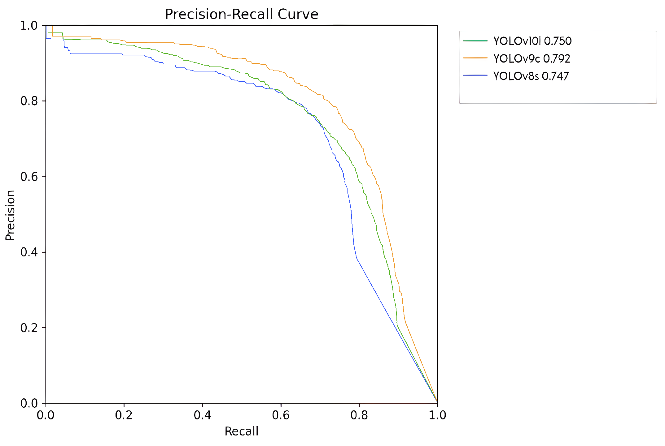
• Training and evaluation. We trained and evaluated multiple machine learning models to detect the lack of nitrogen based on the seedlings morphology and we also trained multiple object detection architectures, including YOLOv8 [48], YOLOv9 [49], and YOLOv10 [50], to detect the lack of potassium based on the lettuces texture.
• Results comparison: In this final step, we compare the results obtained from laboratory tests with those obtained from our system.

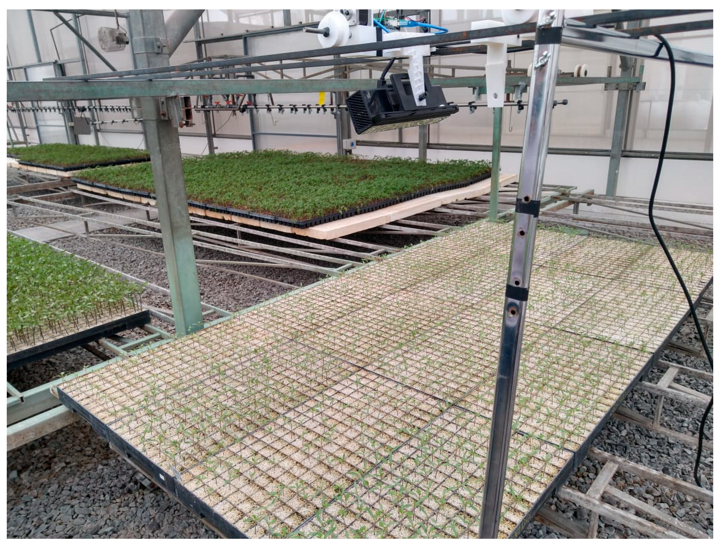
3.1. Data Acquisition

We collected two types of data: images and 3D point clouds using a Kinect v2.0 RGBD sensor mounted on a cart, as shown in Figure 1. The sensor is placed at a height of z = 60 cm relative to the seedling. It moves along the $(x,y)$ axes at programmable distances based on the characteristics of the trays. The x axis has a distance of 4.20 m and the y axis has a distance of 1.70 m. During each movement of 40 cm along x and 30 cm along y, we captured a scan using the RGBD sensor to obtain different viewing angles of the crop.

We captured the data 15 days after germination. This timing allowed the agronomist to determine the crop yield and optimize fertilizer use. The entire crop includes 12 trays with 162 cavities, each containing Rhodena lettuce seedlings, for a total of 1944 cavities with lettuce seedlings.

We also acquired RGB images on the 15th and 28th days after germination at a resolution of 3000 × 3000 pixels, totaling 640 images from the crop. Then, we manually annotated macronutrient deficiency into two categories: healthy and disease.

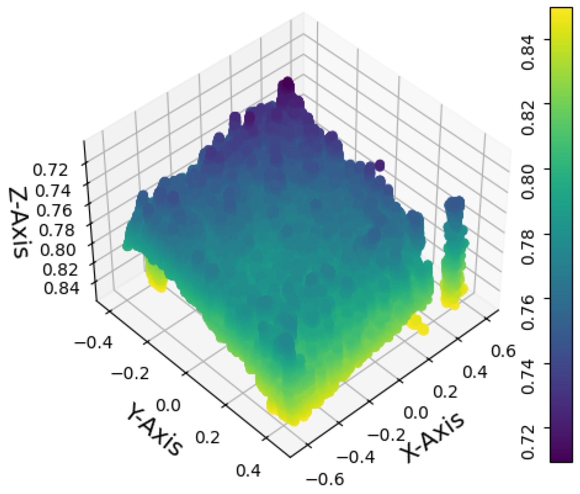
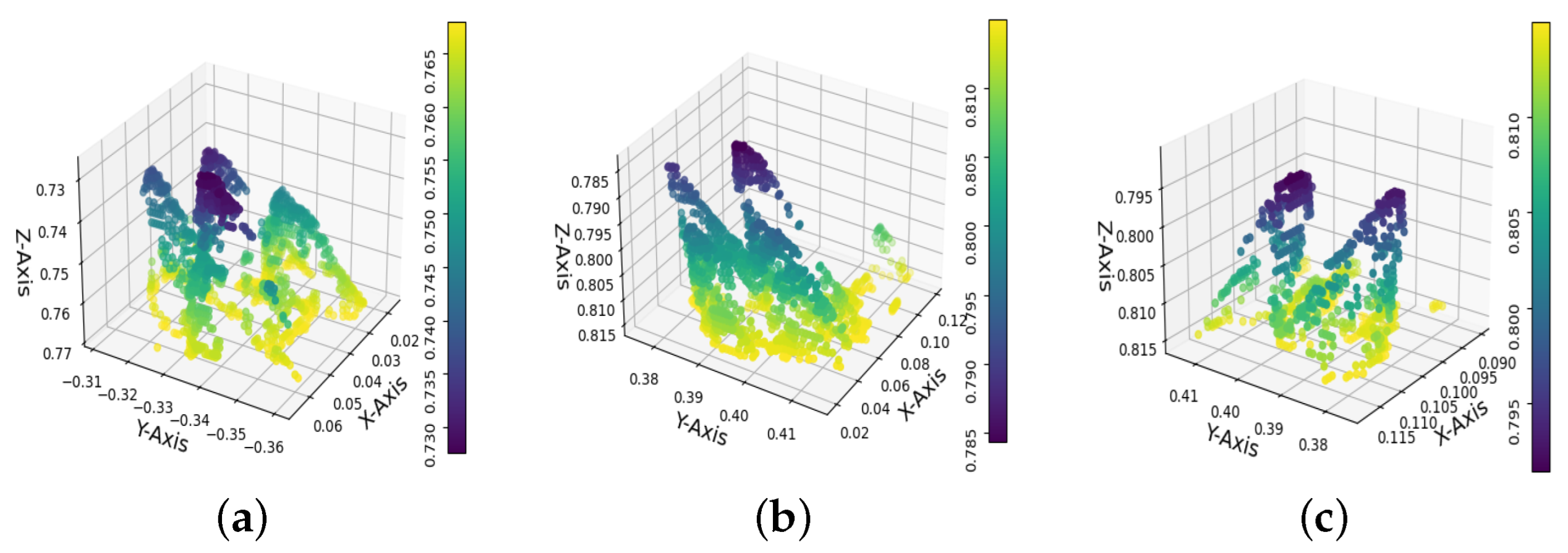
3.2. Point Cloud Registration

Once the 3D scans of the crop were collected, we registered the 3D point clouds using the iterative closest point (ICP) as proposed by Zhang et al. [51]. In this technique, given two point sets, P and Q, the goal is to optimize a rigid transformation on P to align it with Q. ICP solves this problem using an iterative approach that alternates between two steps: correspondence and alignment.

However, the classical ICP is slow to converge to a local minimum due to its linear convergence rate. To address this issue, we used the Anderson acceleration [52]. This approach parameterizes a rigid transformation using another set of variables X, such that any value of X corresponds to a valid rigid transformation, and the ICP iteration can be rewritten as follows:

$$X(k+1)=G_{ICP}\left(X\left(k\right)\right)$$

(1)

Then, Anderson acceleration can be applied to the variable X by performing the following steps in each iteration:

• From the current variable $X\left(k\right)$, recover the rotation matrix $R\left(k\right)$ and translation vector $t\left(k\right)$.
• Perform the ICP update $(R_0,t_0)=G_{ICP}(R\left(k\right),t\left(k\right))$.
• Compute the parameterization of $(R_0,t_0)$ to obtain $G_{ICP}\left(X\left(k\right)\right)$.
• Compute the accelerated value $X_{AA}$ with Anderson acceleration using $X(k-m),\dots$, $X\left(k\right)$ and $G_{ICP}\left(X(k-m)\right),\dots ,G_{ICP}\left(X\left(k\right)\right)$.

Where:

$$X(k+1)AA=G\left(X\left(k\right)\right)-\sum {j=1}^m{\theta }_j^{*}\left(G\left(X\right(k-j+1\left)\right)-G\left(X\right(k-j\left)\right)\right)$$

(2)

The registration process allowed us to apply the methodology proposed in [53] to extract morphological characteristics.

3.3. Detection of Nitrogen Deficiencies

Nitrogen deficiency in crops often leads to stunted growth and reduced biomass. Our system detects this by analyzing the morphology of lettuce seedlings using key morphological characteristics extracted from the registered point cloud.

To extract morphological characteristics, we measure the seedling size, the plant’s germination stage, and the number of leaves and classify them into three stages: first, second, or third.

The height of the crop indicates a nitrogen deficiency, with an average crop height of 3.4 cm. A healthy fertilized seedling reaches an average height of 6 cm, which marks the first stage of growth. The nitrogen element N becomes apparent around day 15 after germination. In the first stage, the average height is 6 cm; in the second stage, the height ranges around 4 cm; in the third stage, the height is less than 3 cm; and the fourth stage corresponds to seedlings that did not germinate.

We annotated a total of 1944 cavities with lettuce seedlings and split the data into $70\%$ for training and $30\%$ for validation.

Then, we trained machine learning classifiers that included a support vector machine (SVM), neighborhood component analysis (NCA), decision tree classifier (DTC), and a linear model with stochastic gradient descent (SGD).

3.4. Detection of Potassium Deficiency

Potassium deficiency usually results in abnormal leaf colorations, such as chlorosis or necrosis. To recognize these visual symptoms, we compared various YOLO [54] models trained to detect and classify characteristic color changes related to potassium deficiency.

YOLO models feature a unified detector that utilizes regression, associated class probabilities, and detection bounding boxes. YOLO utilizes global features, and its main advantage is its speed, allowing real-time detection on standard hardware. In general, the YOLO algorithm can be summarized in three main components:

• Single step grid predictions. It divides the image I into $M\times M$ grid cells, where each cell contains detection predictions.
• Bounding box regression. It determines the bounding boxes, which correspond to the rectangles that contain the objects in the image. The attributes of these bounding boxes are determined using a single regression module as shown in Equation (3).

  $$Y=[p,x,y,h,w,c]$$

  (3)
  Here, Y is the vector representation of each bounding box, p is the probability score of each grid cell containing an object [0, 1], $x,y$ are the coordinates of the center of the bounding box concerning the grid cell, $h,w$ is the height and width of the bounding box to the cell, and c is the class for the n number of classes.
• Nonmaximum suppression (NMS). An object may have several overlapped detections. NMS keeps the predictions with the highest detection confidence.

YOLO drawbacks include the potential failure to detect small objects and less likely prediction of false positives in the background. Early versions were prone to localization errors.

This work compares three of the most recent YOLO models: YOLOv8 [48], YOLOv9 [49], and YOLOv10 [50], described in the following sections.

3.4.1. YOLOv8

The architecture of YOLOv8 is designed to enhance real-time object detection capabilities with improved accuracy and efficiency. YOLOv8 is structured around three main components: the backbone, the neck, and the head. The backbone, which is responsible for feature extraction, utilizes CSPDarknet53, a variant of the Darknet architecture. This version incorporates cross-stage partial (CSP) connections, which improve information flow and gradient propagation during training. The neck of YOLOv8 employs a path aggregation network (PANet) to facilitate multiscale feature fusion, crucial for detecting objects of varying sizes within an image. The head consists of multiple detection heads that predict bounding boxes, class probabilities, and objectness scores, incorporating dynamic anchor assignment and a novel intersection over union (IoU) loss function to enhance detection accuracy and handle overlapping objects more effectively [55]. Figure 4 shows the architecture of YOLOv8.

YOLOv8 also introduces several advancements in training strategies and model variants to cater to different application needs. The model employs adaptive training techniques, including advanced data augmentation methods like MixUp and CutMix, to improve robustness and generalization. Additionally, YOLOv8 supports multiple backbones, such as EfficientNet and ResNet, allowing users to customize the architecture based on specific requirements. The availability of different model variants, such as YOLOv8-tiny and YOLOv8x, provides flexibility in balancing accuracy and computational efficiency [48].

3.4.2. YOLOv9

YOLOv9 represents a significant advancement in the YOLO series, introducing innovative techniques to enhance object detection performance. The architecture of YOLOv9 is built upon the foundation of YOLOv7, with substantial improvements through the integration of two key innovations: programmable gradient information (PGI) and the generalized efficient layer aggregation network (GELAN). PGI addresses the issue of information bottleneck, a common challenge in deep neural networks where crucial data can be lost as they progress through layers. By implementing PGI, YOLOv9 ensures efficient gradient flow and reliable gradient backpropagation, which enhances the model’s learning capabilities and accuracy. This is achieved through an auxiliary reversible branch that provides additional pathways for gradient flow, thereby preserving essential information throughout the training process. Figure 5 shows the architecture of YOLOv9 [49].

GELAN further complements the PGI framework by focusing on efficient layer aggregation and parameter utilization. It combines principles from CSPNet and ELAN to optimize gradient path planning and feature integration, resulting in a lightweight yet robust architecture. This design allows YOLOv9 to maintain high inference speed and accuracy while using fewer parameters and computational resources compared to its predecessors. The architecture supports multiple model variants, such as YOLOv9-S, YOLOv9-M, YOLOv9-C, and YOLOv9-E, catering to different application needs from lightweight to performance-intensive scenarios [56].

3.4.3. YOLOv10

YOLOv10 introduces several architectural innovations that enhance both efficiency and accuracy in real-time object detection. One of the key advancements is the implementation of a consistent dual assignments strategy, which eliminates the need for nonmaximum suppression (NMS) during inference. This approach significantly reduces inference latency while maintaining competitive performance by combining one-to-one and one-to-many label assignments during training [50]. Furthermore, YOLOv10 adopts a holistic model design based on efficiency accuracy, optimizing various components to minimize computational overhead. This includes a lightweight classification head using depth-wise separable convolutions, spatial-channel decoupled downsampling to reduce information loss and computational cost, and a rank-guided block design to efficiently allocate computational resources based on stage redundancy. Figure 6 shows a summarized architecture of YOLOv10.

To further enhance accuracy, YOLOv10 incorporates large-kernel convolutions and a partial self-attention (PSA) module. Large-kernel convolutions expand the receptive field, improving the model’s ability to capture detailed features, particularly beneficial for small object detection. The PSA module integrates global representation learning with minimal computational cost by processing only a portion of the features through multihead self-attention, thus avoiding the overhead associated with full self-attention mechanisms. These architectural improvements allow YOLOv10 to achieve superior performance metrics, such as higher mean average precision (mAP) and reduced latency compared to previous YOLO versions and other state-of-the-art models, making it highly suitable for real-time applications.

3.5. Evaluation Metrics

The metrics used to evaluate potassium deficiencies are precision, recall, and mean average precision (mAP).

Mean average precision (mAP) is a widely used metric for evaluating the performance of object detection models. Combining precision and recall, it provides a comprehensive measure of a model’s ability to detect objects accurately.

Precision measures the fraction of true positive detections out of all positive detections made by the model, and indicates how many of the detected objects are actually correct, as defined in Equation (4).

$$\mathrm{Precision}={\displaystyle \frac{\mathrm{TP}}{\mathrm{TP}+\mathrm{FP}}}$$

(4)

Recall measures the fraction of true positive detections out of all actual objects in the image, and indicates how many of the actual objects were detected by the model, as defined by Equation (5).

$$\mathrm{Recall}={\displaystyle \frac{\mathrm{TP}}{\mathrm{TP}+\mathrm{FN}}}$$

(5)

Intersection over union (IoU) is used to evaluate the accuracy of an object detector by comparing the overlap between the predicted bounding box and the ground truth bounding box. A higher IoU indicates better overlap and, thus, a more accurate detection.

Average precision (AP) is calculated for each class by integrating the area under the precision–recall curve. It provides a single score summarizing the precision–recall trade-off for that class. mAP is calculated by averaging the AP scores over all classes and possibly over different IoU thresholds. This ensures that the evaluation does not rely on a single IoU threshold, which can vary depending on the task and dataset. For example, in the COCO challenge, mAP is calculated by averaging AP over multiple IoU thresholds (from 0.5 to 0.95 in increments of 0.05) across all object classes.

A high mAP score indicates that the model is capable of detecting objects with both high precision and recall, which is crucial for safety and reliability in these applications.

4. Results

The nutritional needs of seedlings in a greenhouse are primarily dependent on the concentration of existing nutrients on the substrate and irrigation. However, the lack of macroelement detection in seedlings, especially lettuce at an early age, allows for appropriate treatment and avoids total loss of production. This work demonstrates that it is possible to match or mimic laboratory tests and proposes the use of AI algorithms to apply only the necessary fertilizers.

There are two types of cycles in cultivation: long and short. The long cycle lasts between 100 and 120 days in winter and 90 to 100 days in autumn. The short cycle lasts between 50 and 70 days in summer and 80 to 90 days in spring. This work was performed in the short spring cycle, which has a relatively warm climate with temperatures close to 30 °C. In addition, the hours of sunlight are longer, directly impacting the development of the seedlings. The greenhouse is located north of Celaya, Guanajuato, Mexico, at latitude $20.613112$ and longitude $-100.921866$, at an altitude of 1756 m above mean sea level.

4.1. Laboratory Tests

The Rhodena lettuce crop was divided into two groups: healthy and diseased. The diseased group, which covered 80% of the crop, was only watered, while the healthy group (the remaining 20%) was watered and fertilized normally. To verify the values of macroelements, a laboratory conducted destructive tests on both groups of seedlings.

Table 1. Test laboratory analysis of macroelement concentrations in Rhodena lettuce seedlings. The table presents the concentrations of multiple elements in parts per million (ppm). The nutritional sufficiency ranges for each element are also provided for reference.

Test Laboratory Lettuce Rhodena
Element	Result		Sufficiency	Unit
	Healthy	Diseased
Nitrogen	4.91	2.05	4.50–5.50	%
Phosphorus	0.47	0.32	0.35–0.40	%
Potassium	6.17	2.75	6.00–7.00	%
Calcium	1.89	0.78	1.00–2.00	%
Magnesium	0.81	1.48	0.30–0.40	%
Sulfur	0.51	0.35	0.20–0.60	%
Iron	1429	3956	50.0–100	ppm
Zinc	76.20	27.49	25.0–100	ppm
Manganese	93.49	51.39	20.0–200	ppm
Copper	6.24	11.25	5.00–10.0	ppm
Boron	52.25	43.28	25.0–80.0	ppm

shows the laboratory tests of the macroelements nitrogen, phosphorus, calcium, magnesium, and sulfur in percentages, as well as iron, zinc, manganese, copper, and boron in units of parts per million (ppm). The table compares healthy seedlings with diseased seedlings, indicating the necessary nutritional requirements for the seedlings.

Figure 7 shows macroelements, where 1 is very low, 2 low, 3 sufficient, 4 high, and 5 very high. The level of 3 is considered sufficient. In this work, we focus on detecting the lack of nitrogen and potassium, which are very low and the most prevalent in the crop.

4.2. Detection of Nitrogen Deficiencies

Using multiple scans taken on the 15th day after germination, we obtain a single point cloud combining multiple scans using ICP, as described in Section 3.2.

Figure 8 shows the alignment of 8 point clouds, each containing 12 trays with 162 cavities. The color variations along the z axis indicate the seedlings’ height, and the gaps represent nongerminated seedlings.

From the registered point cloud, we extract the characteristics of each seedling, which serve as inputs for the classifier. These characteristics encompass leaf count, height, and growth stage.

To obtain the height, we use the algorithm presented in [53]. In this procedure, we normalize the points to the agrolite or substate and obtain the highest point point as $(x,y)$. At the time of the scan, the Rhodena lettuce plant had developed to the second stage of growth. The height is used to determine nitrogen deficiency. The crop has an average height of 3.2 cm, while healthy seedlings have an average height of 4 cm. The seedlings in the first stage are those that have received fertilizer.

The diagram in Figure 9a illustrates the height distribution (in cm) during three different growth stages of Rhodena lettuce. The tallest median height is observed at growth stage 0, while the lowest is seen at growth stage 2. The interquartile ranges vary among stages, indicating differences in height variability. Additionally, Figure 9b displays the distribution of the number of leaves at each growth stage. Growth stage 0 exhibits the highest median number of leaves, while growth stages 1 and 2 have similar median values but lower overall leaf counts.

Figure 10a displays the distribution of plant heights in centimeters. The data show a relatively symmetrical spread with a peak of around 0.04 cm, indicating that most plants fall within this height range. The distribution shows some variability, with heights ranging from approximately 0.02 cm to 0.06 cm. Figure 10b illustrates the distribution of the number of leaves per plant. The distribution is bimodal, with two prominent peaks at 2 and 4 leaves, suggesting that most plants have 2 or 4 leaves, with fewer occurrences of other leaf counts. Figure 10c shows the frequency of plants in different stages of growth (0, 1, and 2). Growth stage 1 has the highest frequency, followed by Stage 2, while Stage 0 has the lowest frequency, indicating the prevalence of plants in intermediate growth stages.

The scatter plots in Figure 11 illustrate the three growth stages of the Rhodena lettuce seedling. In a healthy crop without diseases, most of the seedlings would be at this stage. However, our experiment shows that a high percentage of the monitored crop plants are in the second growth stage. Specifically, Figure 11a displays a lettuce plant with four true leaves and two cotyledons, standing at a height of 4 cm. Figure 11b depicts four leaves, two cotyledons, and two first true leaves with a height of 3 cm. Lastly, Figure 11c shows two cotyledons with a height of 2 cm. The first, second, and third stages represent 5.81%, 53.98%, and 25.45% of the crop, respectively, with the remaining 5.63% representing failures.

We trained multiple machine learning models to classify lettuce seedlings into four categories: first stage, second stage, third stage, and failures. The results of the machine learning classifiers to classify nitrogen deficiencies are shown in

Table 2. Crop production accuracy by growth stage of each classifier production accuracy. The table presents the prediction results of various classifiers, detailing the percentage of lettuce seedlings classified into different growth stages (third, second, first, and failures). The overall production is calculated by summing the percentages across the first, second, and third stages. The accuracy of each classifier is determined by summing the percentages of all stages and failures.

Classifier Crop Production %
Stage	NCA	SGD	DTC	Linear	RBF	Poly
Third	30.1	27.42	25.45	23.49	23.9	22.01
Second	52.13	48.34	53.98	53.65	52.12	53.87
First	1.87	2.18	5.81	2.02	5.95	5.36
Fails	4.94	6.54	5.63	6.03	4.80	6.08
Accuracy	89.04	84.48	90.87	85.19	86.77	87.32
15th day Prod.	84.01	77.94	85.24	79.16	81.97	81.24

. Each cell in the table represents the percentage of seedlings at different stages. The sum of the percentages in the first, second, and third stages indicates the overall production. Adding all stages and failures gives the accuracy of the classifiers. The decision tree classifier (DTC) attained the highest accuracy at 90.87% and a crop production rate of 85.24% on the 15th day. The percentage of seedlings in the third and second stages indicates limited development of the lettuce plant.

4.3. Detection of Potassium Deficiency

Lack of potassium in seedlings can cause yellow marks to appear in the veins of the leaves or on the leaves themselves, usually around day 20 after germination.

We conducted training using manually annotated images to train YOLOv8, YOLOv9, and YOLOv10 models for detecting healthy and diseased categories.

Table 3. Comparison of model accuracy across YOLO versions: The table presents the precision, recall, and mAP50 values for different versions of YOLO models—YOLOv8, YOLOv9, and YOLOv10—trained on a dataset containing manually annotated images with healthy and diseased categories. The highest-performing variant within each YOLO model family is highlighted in bold.

Detector	Model	Precision	Recall	mAP50
YOLOv8	n	0.750	0.701	0.736
	s	0.633	0.782	0.747
	m	0.788	0.658	0.729
		0.786	0.658	0.713
	x	0.627	0.765	0.737
YOLOv9	t	0.670	0.792	0.772
	s	0.702	0.778	0.784
	m	0.653	0.798	0.783
	c	0.701	0.79	0.792
	e	0.66	0.792	0.784
YOLOv10	n	0.739	0.703	0.716
	s	0.731	0.730	0.740
	m	0.800	0.639	0.740
	b	0.775	0.657	0.715
	l	0.679	0.752	0.750
	x	0.764	0.687	0.726

presents the precision, recall, and mAP50 for each model. Specifically, YOLOv9c achieved the highest mAP of 0.792 among the three detectors.

Figure 12 presents the precision/recall curves for the three most proficient neural network models examined in this study. The YOLOv8s model is depicted in blue with an mAP of $74.7\%$, YOLOv10l in green with $75\%$, and YOLOv9c in orange with $79.2\%$. Notably, the YOLOv9c model exhibited the superior performance.

Figure 13 presents the detection results obtained from the YOLOv8s, YOLOv9c, and YOLOv10l models. The initial row illustrates the manually annotated ground truth. Subsequently, the second, third, and fourth rows depict the predictions generated by the YOLOv8s, YOLOv9c, and YOLOv10l models, respectively.

5. Discussion and Conclusions

This study introduces a novel method for detecting micronutrient deficiencies in Rhodena greenhouse-grown lettuces via 2D and 3D analysis. We used a depth camera to capture 3D point clouds to estimate nitrogen deficiencies through morphological variables, while a deep learning detector analyzed 2D images to identify potassium deficiencies.

Conventional methods for detecting nutrient deficiencies predominantly depend on laboratory analyses and visual inspections, which are inherently time-intensive, costly, and susceptible to human error. Our methodology proposes a noninvasive, real-time alternative that markedly diminishes the necessity for laboratory testing. In identifying nitrogen deficiencies, we evaluated several machine learning techniques, with the decision tree classifier (DTC) attaining the highest accuracy at 90.87%. For the detection of potassium deficiencies, YOLOv9c demonstrated an accuracy of 79.20%. These findings emphasize the promise of AI-driven methodologies in agricultural applications.

The capability to precisely identify nutrient deficiencies at an early stage is indispensable for optimizing fertilizer use and ensuring the robust development of crops. The results indicate that the proposed methodology can be effectively utilized for monitoring lettuce crops, potentially diminishing the necessity for excessive fertilizer usage, thereby yielding economic and environmental advantages. Furthermore, this approach is adaptable to other crops, providing a scalable solution for nutrient monitoring across diverse agricultural contexts.

Although the results are promising, this study has limitations. The performance of the model is highly dependent upon the quality of the input data, specifically the resolution of the images and the precision of the point cloud registration. Likewise, the efficacy of the method in varying environmental conditions or with different varieties of lettuce has yet to be comprehensively examined. Future research should aim to evaluate the methodology in diverse settings and with a variety of crops to determine its broader applicability.

Furthermore, the existing system predominantly addresses deficiencies in nitrogen and potassium. Extending the model to identify other macronutrients, such as phosphorus and magnesium, would significantly increase its efficacy. Additionally, the incorporation of IoT devices for continuous monitoring and automated decision-making systems could be investigated to develop a more holistic crop management tool.

References

1. Natesh, H.; Abbey, L.; Asiedu, S. An overview of nutritional and antinutritional factors in green leafy vegetables. Hortic. Int. J. 2017, 1, 58–65. [Google Scholar] [CrossRef]
2. Kumar, D.; Kumar, S.; Shekhar, C. Nutritional components in green leafy vegetables: A review. J. Pharmacogn. Phytochem. 2020, 9, 2498–2502. Available online: https://www.phytojournal.com/archives/2020.v9.i5.12718/nutritional-components-in-green-leafy-vegetables-a-review (accessed on 1 August 2024).
3. Gupta, K.; Barat, G.; Wagle, D.; Chawla, H. Nutrient contents and antinutritional factors in conventional and non-conventional leafy vegetables. Food Chem. 1989, 31, 105–116. [Google Scholar] [CrossRef]
4. Das, R.; Bhattacharjee, C. Chapter 9—Lettuce. In Nutritional Composition and Antioxidant Properties of Fruits and Vegetables; Jaiswal, A.K., Ed.; Academic Press: Cambridge, MA, USA, 2020; pp. 143–157. [Google Scholar] [CrossRef]
5. Medina-Lozano, I.; Bertolín, J.R.; Díaz, A. Nutritional value of commercial and traditional lettuce (Lactuca sativa L.) and wild relatives: Vitamin C and anthocyanin content. Food Chem. 2021, 359, 129864. [Google Scholar] [CrossRef]
6. Shi, M.; Gu, J.; Wu, H.; Rauf, A.; Emran, T.B.; Khan, Z.; Mitra, S.; Aljohani, A.S.M.; Alhumaydhi, F.A.; Al-Awthan, Y.S.; et al. Phytochemicals, Nutrition, Metabolism, Bioavailability, and Health Benefits in Lettuce—A Comprehensive Review. Antioxidants 2022, 11, 1158. [Google Scholar] [CrossRef]
7. Faran, M.; Nadeem, M.; Manful, C.F.; Galagedara, L.; Thomas, R.H.; Cheema, M. Agronomic Performance and Phytochemical Profile of Lettuce Grown in Anaerobic Dairy Digestate. Agronomy 2023, 13, 182. [Google Scholar] [CrossRef]
8. Frasetya, B.; Harisman, K.; Ramdaniah, N.A.H. The effect of hydroponics systems on the growth of lettuce. IOP Conf. Ser. Mater. Sci. Eng. 2021, 1098, 042115. [Google Scholar] [CrossRef]
9. Majid, M.; Khan, J.N.; Ahmad Shah, Q.M.; Masoodi, K.Z.; Afroza, B.; Parvaze, S. Evaluation of hydroponic systems for the cultivation of Lettuce (Lactuca sativa L., var. longifolia) and comparison with protected soil-based cultivation. Agric. Water Manag. 2021, 245, 106572. [Google Scholar] [CrossRef]
10. Sularz, O.; Smoleń, S.; Koronowicz, A.; Kowalska, I.; Leszczyńska, T. Chemical Composition of Lettuce (Lactuca sativa L.) Biofortified with Iodine by KIO3, 5-Iodo-, and 3.5-Diiodosalicylic Acid in a Hydroponic Cultivation. Agronomy 2020, 10, 1022. [Google Scholar] [CrossRef]
11. Mujiono, M.; Suyono, S.; Purwanto, P. Growth and Yield of Lettuce (Lactuca sativa L.) Under Organic Cultivation. Planta Trop. 2017, 5, 127–131. [Google Scholar] [CrossRef]
12. Cova, A.M.W.; Freitas, F.T.O.d.; Viana, P.C.; Rafael, M.R.S.; Azevedo, A.D.d.; Soares, T.M. Content of inorganic solutes in lettuce grown with brackish water in different hydroponic systems. Rev. Bras. Eng. Agríc. Ambient. 2017, 21, 150–155. [Google Scholar] [CrossRef]
13. Jose, V.; Gino, A.; Noel, O. Humus líquido y microorganismos para favorecer la producción de lechuga (Lactuca sativa var. crespa) en cultivo de hidroponía. J. Selva Andin. Biosph. 2016, 4, 71–83. Available online: http://www.scielo.org.bo/scielo.php?script=sci_arttext&pid=S2308-38592016000200004&nrm=iso (accessed on 1 August 2024). [CrossRef]
14. Monge, C.; Chaves, C.; Arias, M.L. Comparación de la calidad bacteriológica de la lechuga (Lactuca sativa) producida en Costa Rica mediante cultivo tradicional, orgánico o hidropónico. Arch. Latinoam. Nutr. Super. 2011, 61, 69–73. Available online: http://ve.scielo.org/scielo.php?script=sci_arttext&pid=S0004-06222011000100009&nrm=iso (accessed on 1 August 2024).
15. Saah, K.J.A.; Kaba, J.S.; Abunyewa, A.A. Inorganic nitrogen fertilizer, biochar particle size and rate of application on lettuce (Lactuca sativa L.) nitrogen use and yield. All Life 2022, 15, 624–635. [Google Scholar] [CrossRef]
16. Dávila Rangel, I.E.; Trejo Téllez, L.I.; Ortega Ortiz, H.; Juárez Maldonado, A.; González Morales, S.; Companioni González, B.; Cabrera De la Fuente, M.; Benavides Mendoza, A. Comparison of Iodide, Iodate, and Iodine-Chitosan Complexes for the Biofortification of Lettuce. Appl. Sci. 2020, 10, 2378. [Google Scholar] [CrossRef]
17. Liu, Q.; Huang, L.; Chen, Z.; Wen, Z.; Ma, L.; Xu, S.; Wu, Y.; Liu, Y.; Feng, Y. Biochar and its combination with inorganic or organic amendment on growth, uptake and accumulation of cadmium on lettuce. J. Clean. Prod. 2022, 370, 133610. [Google Scholar] [CrossRef]
18. Ahmed, Z.F.R.; Alnuaimi, A.K.H.; Askri, A.; Tzortzakis, N. Evaluation of Lettuce (Lactuca sativa L.) Production under Hydroponic System: Nutrient Solution Derived from Fish Waste vs. Inorganic Nutrient Solution. Horticulturae 2021, 7, 292. [Google Scholar] [CrossRef]
19. Anisuzzaman, M.; Rafii, M.Y.; Jaafar, N.M.; Izan Ramlee, S.; Ikbal, M.F.; Haque, M.A. Effect of Organic and Inorganic Fertilizer on the Growth and Yield Components of Traditional and Improved Rice (Oryza sativa L.) Genotypes in Malaysia. Agronomy 2021, 11, 1830. [Google Scholar] [CrossRef]
20. El-Mogy, M.M.; Abdelaziz, S.M.; Mahmoud, A.W.M.; Elsayed, T.R.; Abdel-Kader, N.H.; Mohamed, M.I.A. Comparative Effects of Different Organic and Inorganic Fertilisers on Soil Fertility, Plant Growth, Soil Microbial Community, and Storage Ability of Lettuce. Agric. (Pol’nohospodárstvo) 2020, 66, 87–107. [Google Scholar] [CrossRef]
21. Zhang, E.; Lin, L.; Liu, J.; Li, Y.; Jiang, W.; Tang, Y. The effects of organic fertilizer and inorganic fertilizer on yield and quality of lettuce. Adv. Eng. Res. 2022, 129, 624–635. [Google Scholar] [CrossRef]
22. Pavlou, G.C.; Ehaliotis, C.D.; Kavvadias, V.A. Effect of organic and inorganic fertilizers applied during successive crop seasons on growth and nitrate accumulation in lettuce. Sci. Hortic. 2007, 111, 319–325. [Google Scholar] [CrossRef]
23. Kutyauripo, I.; Rushambwa, M.; Chiwazi, L. Artificial intelligence applications in the agrifood sectors. J. Agric. Food Res. 2023, 11, 100502. [Google Scholar] [CrossRef]
24. Rameshwari, D. Classification of Macronutrient Deficiencies in Maize Plant using Machine Learning. Int. J. Res. Appl. Sci. Eng. Technol. 2021, 9, 4321–4326. [Google Scholar] [CrossRef]
25. Raju, S.H.; Adinarayna, S.; Prasanna, N.M.; Jumlesha, S.; Sesadri, U.; Hema, C. Nutrient Deficiency Detection using a MobileNet: An AI-based Solution. In Proceedings of the 2023 7th International Conference on I-SMAC (IoT in Social, Mobile, Analytics and Cloud) (I-SMAC), Kirtipur, Nepal, 11–13 October 2023; pp. 609–615. [Google Scholar] [CrossRef]
26. Krishna, V.; Raju, Y.D.S.; Raghavendran, C.V.; Naresh, P.; Rajesh, A. Identification of Nutritional Deficiencies in Crops Using Machine Learning and Image Processing Techniques. In Proceedings of the 2022 3rd International Conference on Intelligent Engineering and Management (ICIEM), London, UK, 27–29 April 2022; pp. 925–929. [Google Scholar] [CrossRef]
27. Suleiman, R.F.R.; Riduwan, M.K.; Kamal, A.N.M.; Wahab, N.A. Soil Nutrient Deficiency Detection of Lime Trees using Signal-based Deep Learning. In Proceedings of the 2022 International Visualization, Informatics and Technology Conference (IVIT), Kuala Lumpur, Malaysia, 1–2 November 2022; pp. 261–265. [Google Scholar] [CrossRef]
28. J, A.; K, M.; K, V. Plant Nutrient Deficiency Detection and Classification—A Review. In Proceedings of the 2023 5th International Conference on Inventive Research in Computing Applications (ICIRCA), Coimbatore, India, 3–5 August 2023; pp. 796–802. [Google Scholar] [CrossRef]
29. Sudhakar, M.; Priya, R.M.S. Computer Vision Based Machine Learning and Deep Learning Approaches for Identification of Nutrient Deficiency in Crops: A Survey. Nat. Environ. Pollut. Technol. 2023, 22, 1387–1399. [Google Scholar] [CrossRef]
30. Kok, Z.H.; Shariff, A.R.M.; Khairunniza-Bejo, S.; Kim, H.T.; Ahamed, T.; Cheah, S.S.; Wahid, S.A.A. Plot-Based Classification of Macronutrient Levels in Oil Palm Trees with Landsat-8 Images and Machine Learning. Remote Sens. 2021, 13, 2029. [Google Scholar] [CrossRef]
31. Sabri, N.; Kassim, N.S.; Ibrahim, S.; Roslan, R.; Mangshor, N.N.A.; Ibrahim, Z. Nutrient deficiency detection in Maize (Zea mays L.) leaves using image processing. IAES Int. J. Artif. Intell. (IJ-AI) 2020, 9, 304. [Google Scholar] [CrossRef]
32. Rahadiyan, D.; Hartati, S.; Nugroho, A. An Overview of Identification and Estimation Nutrient on Plant Leaves Image Using Machine Learning. J. Theor. Appl. Inf. Technol. 2022, 100, 1836–1852. Available online: https://www.jatit.org/volumes/Vol100No6/20Vol100No6.pdf (accessed on 1 August 2024).
33. Sowmiya, M.; Krishnaveni, S. Deep Learning Techniques to Detect Crop Disease and Nutrient Deficiency—A Survey. In Proceedings of the 2021 International Conference on System, Computation, Automation and Networking (ICSCAN), Puducherry, India, 30–31 July 2021; pp. 1–5. [Google Scholar] [CrossRef]
34. Kamelia, L.; Rahman, T.K.A.; Saragih, H.; Uyun, S. Survey on Hybrid Techniques in The Classification of Nutrient Deficiency Levels in Citrus Leaves. In Proceedings of the 2021 7th International Conference on Wireless and Telematics (ICWT), Bandung, Indonesia, 19–20 August 2021; pp. 1–4. [Google Scholar] [CrossRef]
35. Arun, K.S.; Huang, T.S.; Blostein, S.D. Least-squares fitting of two 3-D point sets. IEEE Trans. Pattern Anal. Mach. Intell. 1987, 9, 698–700. [Google Scholar] [CrossRef]
36. Besl, P.J.; McKay, N.D. Method for registration of 3-D shapes. In Proceedings of the Robotics’91: Sensor Fusion IV: Control Paradigms and Data Structures, Boston, MA, USA, 14–15 November 1991; SPIE: Bellingham, WA, USA, 1992; Volume 1611, pp. 586–606. [Google Scholar] [CrossRef]
37. Chen, Y.; Medioni, G. Object modelling by registration of multiple range images. Image Vis. Comput. 1992, 10, 145–155. [Google Scholar] [CrossRef]
38. Zhang, Z. Iterative point matching for registration of free-form curves and surfaces. Int. J. Comput. Vis. 1994, 13, 119–152. [Google Scholar] [CrossRef]
39. Zhang, K.; Chen, H.; Wu, H.; Zhao, X.; Zhou, C. Point cloud registration method for maize plants based on conical surface fitting—ICP. Sci. Rep. 2022, 12, 6852. [Google Scholar] [CrossRef] [PubMed]
40. Amritraj, S.; Hans, N.; Pretty, C.; Cyril, D. An Automated and Fine- Tuned Image Detection and Classification System for Plant Leaf Diseases. In Proceedings of the 2023 International Conference on Recent Advances in Electrical, Electronics, Ubiquitous Communication, and Computational Intelligence (RAEEUCCI), Chennai, India, 19–21 April 2023; pp. 1–5. [Google Scholar] [CrossRef]
41. Pandey, P.; Patra, R. A Real-time Web-based Application for Automated Plant Disease Classification using Deep Learning. In Proceedings of the 2023 IEEE International Symposium on Smart Electronic Systems (iSES), Ahmedabad, India, 18–20 December 2023; pp. 230–235. [Google Scholar] [CrossRef]
42. Nabaasa, E.; Natumanya, D.; Grace, B.; Kiwanuka, C.N.; Muhunga, K.B.J. A Model for Detecting the Presence of Pesticide Residues in Edible Parts of Tomatoes, Cabbages, Carrots, and Green Pepper Vegetables. In Proceedings of the Artificial Intelligence and Applications, Toronto, ON, Canada, 20–21 July 2024; Volume 2, pp. 225–232. [Google Scholar] [CrossRef]
43. Li, H.; Gu, Z.; He, D.; Wang, X.; Huang, J.; Mo, Y.; Li, P.; Huang, Z.; Wu, F. A lightweight improved YOLOv5s model and its deployment for detecting pitaya fruits in daytime and nighttime light-supplement environments. Comput. Electron. Agric. 2024, 220, 108914. [Google Scholar] [CrossRef]
44. Bello, R.W.; Oladipo, M.A. Mask YOLOv7-based drone vision system for automated cattle detection and counting. Artif. Intell. Appl. 2024, 2, 129–139. [Google Scholar] [CrossRef]
45. Broadley, M.; Escobar-Gutierrez, A.; Burns, A.; Burns, I. What are the effects of nitrogen deficiency on growth components of lettuce? New Phytol. 2000, 147, 519–526. [Google Scholar] [CrossRef]
46. Yang, R.; Wu, Z.; Fang, W.; Zhang, H.; Wang, W.; Fu, L.; Majeed, Y.; Li, R.; Cui, Y. Detection of abnormal hydroponic lettuce leaves based on image processing and machine learning. Inf. Process. Agric. 2023, 10, 1–10. [Google Scholar] [CrossRef]
47. Gao, H.; Mao, H.; Ullah, I. Analysis of metabolomic changes in lettuce leaves under low nitrogen and phosphorus deficiencies stresses. Agriculture 2020, 10, 406. [Google Scholar] [CrossRef]
48. Terven, J.; Córdova-Esparza, D.M.; Romero-González, J.A. A comprehensive review of yolo architectures in computer vision: From yolov1 to yolov8 and yolo-nas. Mach. Learn. Knowl. Extr. 2023, 5, 1680–1716. [Google Scholar] [CrossRef]
49. Wang, C.Y.; Yeh, I.H.; Liao, H.Y.M. YOLOv9: Learning What You Want to Learn Using Programmable Gradient Information. arXiv 2024, arXiv:2402.13616. [Google Scholar]
50. Wang, A.; Chen, H.; Liu, L.; Chen, K.; Lin, Z.; Han, J.; Ding, G. YOLOv10: Real-Time End-to-End Object Detection. arXiv 2024, arXiv:2405.14458. [Google Scholar]
51. Zhang, J.; Yao, Y.; Deng, B. Fast and Robust Iterative Closest Point. IEEE Trans. Pattern Anal. Mach. Intell. 2021, 44, 3450–3466. [Google Scholar] [CrossRef]
52. Anderson, D.G. Iterative procedures for nonlinear integral equations. J. ACM 1965, 12, 547–560. [Google Scholar] [CrossRef]
53. González-Barbosa, J.J.; Ramírez-Pedraza, A.; Ornelas-Rodríguez, F.J.; Cordova-Esparza, D.M.; González-Barbosa, E.A. Dynamic Measurement of Portos Tomato Seedling Growth Using the Kinect 2.0 Sensor. Agriculture 2022, 12, 449. [Google Scholar] [CrossRef]
54. Redmon, J.; Divvala, S.; Girshick, R.; Farhadi, A. You Only Look Once: Unified, Real-Time Object Detection. arXiv 2016, arXiv:1506.02640. [Google Scholar]
55. Torres, J. YOLOv8 Architecture: A Deep Dive into its Architecture. 2024. Available online: https://yolov8.org/yolov8-architecture/ (accessed on 14 August 2024).
56. Mukherjee, S. YOLOv9: Exploring Object Detection with YOLO Model. 2024. Available online: https://blog.paperspace.com/yolov9-2/ (accessed on 14 August 2024).
Figure 1. ScanSeedling v2.0: prototype scan of entire crops. The sensor moves along the x-axis to 2 m, the y-axis to 6 m, and the z-axis to a height of 0.60 m.
Agriengineering 06 00198 g001
Figure 2. Diseases seedling Rhodena lettuce. Panel (a) shows nitrogen deficiencies, and (b,c) show potassium (K) deficiencies.
Agriengineering 06 00198 g002
Figure 3. Overview of the proposed methodology for detecting macronutrient deficiencies in Rhodena lettuce seedlings. The top row illustrates the steps for 2D data analysis, which focuses on detecting potassium deficiencies using object detection models. The bottom row shows the steps for 3D data analysis, which are used to detect nitrogen deficiencies through morphological feature extraction and machine learning classifiers.
Agriengineering 06 00198 g003
Figure 4. YOLOv8 network architecture: The diagram illustrates the structure of YOLOv8, divided into three main components: backbone, head, and output. The backbone is responsible for feature extraction and includes multiple convolutional (Conv) and C2f layers, along with a spatial pyramid pooling-fast (SPPF) block. The head performs feature aggregation and enhancement through multiple concatenation (Concat) and upsampling (U) operations, followed by additional C2f layers. Finally, the output section applies detection layers to produce the final object detection results.
Agriengineering 06 00198 g004
Figure 5. YOLOv9 programmable gradient information (PGI) architecture. The model is composed of an auxiliary reversible branch (left), a main processing branch (center), and a multilevel auxiliary information module (right). The auxiliary reversible branch utilizes a series of AB (auxiliary block) modules, while the main processing branch consists of MB (main block) modules. The multilevel auxiliary information module combines outputs from both branches and incorporates PH (pooling head) modules to integrate and process multiscale features. PGI enables dynamic information flow across different levels of the network, facilitating efficient detection and classification tasks.
Agriengineering 06 00198 g005
Figure 6. YOLOv10 NMS-free architecture with one-to-many matching. YOLOv10 eliminates the need for nonmaximum suppression (NMS) by incorporating a dual-label assignment framework. The backbone network extracts image features, which are processed by the path aggregation network (PAN). The model utilizes two heads: a one-to-one head for precise regression and classification, and a one-to-many head designed to handle a broader range of object sizes. The consistent match metric (CMM) ensures that the model consistently matches detected objects across different scales, enhancing the accuracy and robustness of detections.
Agriengineering 06 00198 g006
Figure 7. Comparative analysis of macroelement levels in healthy and diseased Rhodena lettuce seedlings. The bar chart categorizes macroelement concentrations into five levels: 1 (very low), 2 (low), 3 (sufficient), 4 (high), and 5 (very high), with level 3 indicating sufficiency. The analysis highlights that nitrogen (N) and potassium (K) are at very low levels, particularly in diseased seedlings.
Agriengineering 06 00198 g007
Figure 8. Point clouds registration. The image shows the whole crop area. The colors along the z axis represent the height of the seedlings, while the gaps reveal the seedlings that did not germinate.
Agriengineering 06 00198 g008
Figure 9. Heights and leaves distribution across development stages. Panel (a) shows the height distribution (in cm) of lettuces at different growth stages (0, 1, and 2). Height decreases progressively from Stage 0 to Stage 2. (b) Bar plot showing the number of leaves at each growth stage, with Stage 0 having the most leaves, and Stages 1 and 2 showing similar and lower leaf counts.
Agriengineering 06 00198 g009
Figure 10. Distribution of morphological measurements and grown stages. (a) shows an histogram of plant height distribution in centimeters, showing a peak around 0.04 cm with a broad spread from 0.02 cm to 0.06 cm. (b) Histogram of the distribution of the number of leaves, highlighting two prominent peaks at 2 and 4 leaves. (c) Bar plot showing the distribution of growth stages.
Agriengineering 06 00198 g010
Figure 11. Developmental phases of lettuce. Panel (a) exhibits four true leaves, two cotyledons, and a height of 4 cm. Panel (b) presents two true leaves and two cotyledons with a height of 3 cm. Panel (c) displays two cotyledons with a height of 2 cm. According to the DTC technique, optimal results were achieved by delineating the plant morphology for each growth stage with an accuracy of 90.87% and a production forecast of 85.24%.
Agriengineering 06 00198 g011
Figure 12. Precision/recall curves corresponding to the evaluation of the three most effective models.
Agriengineering 06 00198 g012
Figure 13. Potassium deficiency detection. The first row displays manually labeled ground truth detections. The second, third, and fourth rows present the predictions for YOLOv8s, YOLOv9c, and YOLOv10l, respectively.
Agriengineering 06 00198 g013