Soil Moisture Spatial Variability and Water Conditions of Coffee Plantation

Abstract

Remotely piloted aircraft (RPA) are essential in precision coffee farming due to their capability for continuous monitoring, rapid data acquisition, operational flexibility at various altitudes and resolutions, and adaptability to diverse terrain conditions. This study evaluated the soil water conditions in a coffee plantation using remotely piloted aircraft to obtain multispectral images and vegetation indices. Fifteen vegetation indices were chosen to evaluate the vigor, water stress, and health of the crop. Soil samples were collected to measure gravimetric and volumetric moisture at depths of 0–10 cm and 10–20 cm. Data were collected at thirty georeferenced sampling points within a 1.2 ha area using GNSS RTK during the dry season (August 2020) and the rainy season (January 2021). The highest correlation (51.57%) was observed between the green spectral band and the 0–10 cm volumetric moisture in the dry season. Geostatistical analysis was applied to map the spatial variability of soil moisture, and the correlation between vegetation indices and soil moisture was evaluated. The results revealed a strong spatial dependence of soil moisture and significant correlations between vegetation indices and soil moisture, highlighting the effectiveness of RPA and geostatistics in assessing water conditions in coffee plantations. In addition to soil moisture, vegetation indices provided information about plant vigor, water stress, and general crop health.

1. Introduction

Coffee is one of the most widely consumed beverages worldwide. Brazil is the largest global producer and exporter and the second largest consumer [1]. The estimate from Conab [2] for the Brazilian coffee harvest in 2025 is 51.8 million bags, representing a 4.4% reduction compared with 2024. This decline is attributed to adverse climatic conditions, such as water scarcity and high temperatures, which affected flowering and consequently reduced productivity. Compared with the 2023 harvest, also a low biennial year, the drop is 5.9%. The total area allocated to coffee cultivation will grow by 0.5%, totaling 2.25 million hectares. However, the area in production will decrease by 1.5%, reaching 1.85 million hectares, while the fields in formation will increase by 10.7%, reaching 391.46 thousand hectares [2].

Coffee production is highly sensitive to climatic variations, which directly affect its productivity and quality [3,4,5]. Between 2021 and 2024, South American production fell by 7.6%, the largest reduction since 2004/05, according to the International Coffee Organization (ICO) [6]. In Minas Gerais, the main state producing arabica coffee, the scarcity and irregularity of rainfall have compromised biennial productivity. According to Conab [2], the 2025 harvest was estimated at 34.68 million bags, a reduction of 12.4% compared with the previous year. Productivity also dropped by 11.0%, reaching 23.4 bags per hectare.

Given this scenario, soil attributes, such as moisture, are fundamental for coffee cultivation, directly influencing growth and productivity [7]. Studies on the effects of irrigation on coffee production and development indicate that water application can either accelerate or delay fruit maturation [8,9]. Beverage quality is associated with uniform maturation, which depends on flowering synchronization and proper irrigation management, avoiding water stress during critical grain formation phases [10]. Soil water scarcity can reduce the number of reproductive nodes, compromising flower and fruit formation.

However, water movement in the soil is heterogeneous and influenced by factors such as climate, soil type, topography, and vegetation cover, resulting in significant spatial and temporal variability [11,12]. Studies by [13] demonstrate that creating soil moisture distribution maps using interpolation techniques allows for more efficient irrigation management, increasing productivity and reducing waste. Additionally, according to [14], spatial and temporal variations in soil moisture can be integrated into precision irrigation management.

A comprehensive understanding of the spatial and temporal variability of soil moisture is crucial for optimizing water management in coffee cultivation. To quantify coffee plants’ water needs, adopting precision agriculture (PA) technologies has proven to be an effective strategy. The application of precision agriculture (PA) techniques and tools in coffee cultivation remains relatively recent, particularly in the assessment of soil and plant heterogeneity [15]. Studies such as those by [16], which analyzed the spatial variability of soil moisture through gravimetric moisture, and studies by [15], which investigated the spatial variability of soil fertility and productivity in coffee crops, exemplify this application.

Remote sensing and remotely piloted aircraft (RPA) have been extensively utilized to evaluate soil and plant attribute variability, offering advantages such as ease of data acquisition, enhanced operational flexibility, and greater reliability compared with traditional methods [17,18]. These technologies employ reflectance spectroscopy-based sensors to measure electromagnetic radiation reflected after interacting with various surfaces at specific wavelengths, such as near-infrared and mid-infrared [19]. This reflection generates spectral bands, allowing the extraction of vegetation indices, which are essential for agricultural monitoring [20,21].

In agricultural fields, each surface uniquely reflects electromagnetic radiation, presenting a specific spectral signature. Water and soil have reflectance peaks in the near-infrared wavelength, while vegetation emits radiation in this range and absorbs radiation in the visible spectrum band. In the mid-infrared wavelength, spectral behavior is influenced by water presence in the leaves [22]. Plant chlorophylls exhibit absorption peaks in the blue and red regions of the spectrum, making the red spectral band a key component of remote sensing applications This facilitates the application of indices such as NDVI (normalized difference vegetation index), described by Rouse et al. (1973) [23], and the CIrededge index, described by Gitelson [24]. Additionally, the normalized difference water index (NDWI), introduced by McFeeters [25], is extensively utilized for soil moisture estimation.

Numerous studies emphasize the application of vegetation indices in coffee cultivation [26,27]. Despite the large volume of research on using multispectral images obtained by RPA in coffee plantations, only [28] has evaluated plant water conditions through the leaf water potential attribute.

Thus, this study aims to evaluate the spatial variability of soil moisture and explore possible correlations between this attribute and vegetation indices obtained from high-resolution images to assess the water status of coffee plants.

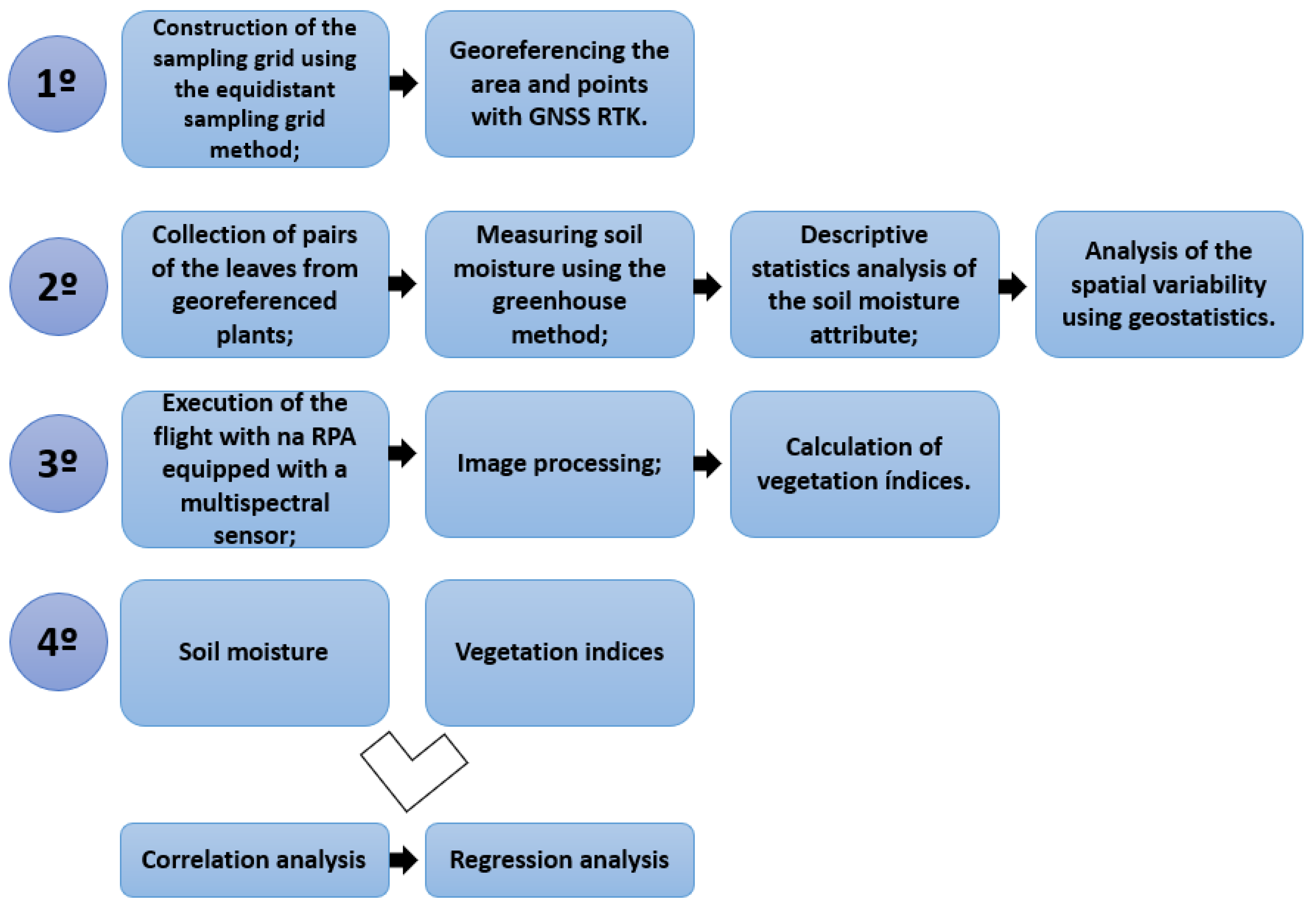
2. Materials and Methods

The research workflow (Figure 1) was divided into four stages. The first stage involved the construction of the sampling mesh and the georeferencing of the area and collection points. The second stage involved collecting soil samples from georeferenced plants to determine soil moisture (gravimetric and volumetric moisture). The third stage involved conducting a flight with a multispectral sensor mounted on the RPA. The final stage involved carrying out correlation and linear regression analysis between soil moisture and vegetation indices calculated using multispectral bands.

2.1. Crop Characterization

The study site (Figure 2) consisted of a 1.2 ha coffee plantation of the species Coffea arabica, specifically the Topázio MG1190 cultivar. The spacing between coffee rows was 3.70 m and between plants 0.70 m. The area is located in the municipality of Três Pontas, the southern region of the state of Minas Gerais, at 905 m altitude and with UTM coordinates S7640030.4 and E449531.5, zone 23K.

According to the Köppen–Geiger climate classification, the region has a Cwb climate. This climate type is characterized as a high-altitude temperate or tropical highland climate, with dry winters (temperatures below 18 °C) and mild summers (temperatures below 23 °C). It generally occurs in regions with altitudes above 900 m. Therefore, the Cwb classification reflects climatic conditions marked by wetter summers and dry winters, typical of higher altitude areas in Brazil.

The same study area was evaluated in the works of [15,29]. The authors also aimed to analyze the correlation between vegetation indices and attributes related to coffee trees. However, none of these studies explored the application of soil moisture in assessing the water status of coffee plants.

2.2. Georeferencing and Sampling

Using QGIS software version 3.4.8, a sampling grid was created with 30 points (Figure 3) at a density of 25 points per hectare. The area and sampling points were subsequently georeferenced using GNSS RTK. The sampling neighborhood affects interpolation accuracy and should be considered when developing maps, as highlighted by [30]. Soil moisture, being an attribute susceptible to changes due to anthropogenic activities, requires a sampling density that adequately represents the variability of the soil property. However, the feasibility of adopting a high sampling density across the entire area was limited, as the sample collection process is labor-intensive and laboratory analyses are costly.

The equidistant sampling grid methodology for precision coffee farming, as proposed by [30], was employed in the construction of the sampling grid. This method aimed to optimize movements within the study area by defining walking routes. In total, 30 points were sampled, with distances ranging from 6 m (minimum) to 175 m (maximum).

In this experiment, each of the 30 sampling points corresponded to an individual plant, which was numerically identified. To assess the water status of the coffee trees, two sampling campaigns were conducted:

• August 2020 (dry season).
• January 2021 (rainy season).

Table 1. Climatic conditions and water balance during the dry and rainy seasons.

Season	Monthly Mean Temperature (°C)	Monthly Mean Relative Moisture (%)	Monthly Accumulated Precipitation (mm)	Mean Wind Speed (m/s)	Water Balance
					PET	SWS	EXC	WD
Dry (Aug/2020)	18.3 *	59.3 *	17.6 *	2.0 *	53.8 *	0.0 *	0.0 *	94.1 *
Rainy (Jan/2021)	23.0 *	70.9 *	270.6 *	1.7 *	110.0 *	39.9 *	212.9 *	0.0 *

PET—potential evapotranspiration, SWS—soil water storage, EXC—excess water and WD—water deficit. * Source: INMET (2020, 2021); Foundation PROCAFE (2020, 2021).

presents climatological data for August 2020 and January 2021, corresponding to the sampling period, along with water balance information. The table was constructed based on data from the National Institute of Meteorology (INMET is the acronym in Portuguese) and the Phytosanitary Bulletins of the Procafé Foundation.

Table 2. Altitude and soil properties.

Parameter	Value
Altitude range (m)	917–935
Elevation variation (m)	18
Soil texture	clayey
Clay (%)	36–38
Silt (%)	32–33
Sand (%)	29–32
Organic matter (%)	2.08–3.38
Ph (KCl)	6.23–8.11
Cation exchange capacity (cmol/dm3)	6.0
Base saturation (%)	69.56–74.16

represents the altitude range among the sampling points and the soil properties of the study area.

Figure 4 illustrates soil water storage levels, highlighting different absorption and water deficit zones for plants.

2.3. Obtaining Soil Moisture

Soil samples were collected from 30 sampling points (Figure 3). At each point, samples were taken at depths of 0–10 cm and 10–20 cm. The samples were removed from the soil using volumetric rings (metal rings with a known volume), which were penetrated into the soil with the aid of an auger. These samples were properly labeled, wrapped in plastic film, and stored in a thermal box to prevent moisture loss before being sent to a soil analysis laboratory.

In the laboratory, following the NBR 6457/2016 [31] protocol, samples were weighed on a precision scale to determine wet mass, then placed in an oven at 105 °C for 24 h. After this period, the samples were weighed again. After determining the dry mass, it was possible to obtain the values of gravimetric moisture (GM) and soil density (SD) using Equations (1) and (2), respectively.

$${GM}_{g/g}={\displaystyle \frac{moistsoil-drysoil}{drysoil}}$$

(1)

$${SD}_{{\displaystyle \frac{g}{c{m}^3}}}={\displaystyle \frac{drysoil}{volumetricring}}$$

(2)

The volumetric moisture (VM) of the soil is defined as the volume of water contained in a given volume of soil sample. It can also be related to gravimetric moisture. According to [32], a mathematical equation (Equation (3)) is applied to convert soil moisture from a mass-based to a volume-based measurement. The product of the multiplication of the gravimetric moisture values by the soil density, divided by water density, gives rise to moisture based on volume, expressed in m³ of water/m³ of soil, cm³/cm³, or mm³/mm³.

$${Vm}_{{\displaystyle \frac{c{m}^3}{c{m}^3}}}={\displaystyle \frac{GM\times SD}{WD}}$$

(3)

where GM is the gravimetric moisture (g/g), SD is the soil density (g/cm³), and WD is the water density (g/cm³).

2.4. Statistical Analysis

After collecting soil moisture data in the field and conducting laboratory analyses, the samples were evaluated in two stages: descriptive statistics and statistical analysis.

2.4.1. Descriptive Statistics

Before performing the geostatistical analysis, the data underwent descriptive analysis to characterize the variability of soil moisture samples. Descriptive statistics, including the minimum (Min), maximum (Max), median (Md), mean, variance (Var), standard deviation (SD), and coefficient of variation (CV), were employed to analyze the data. The CV was classified according to [33], considering variability as low when below 12%, moderate between 12% and 60%, and high when above 60%. This classification allowed for a more precise assessment of attribute variability, essential for understanding soil heterogeneity in the study area. The analyses were conducted using the open-access software R version 4.3.1 [34].

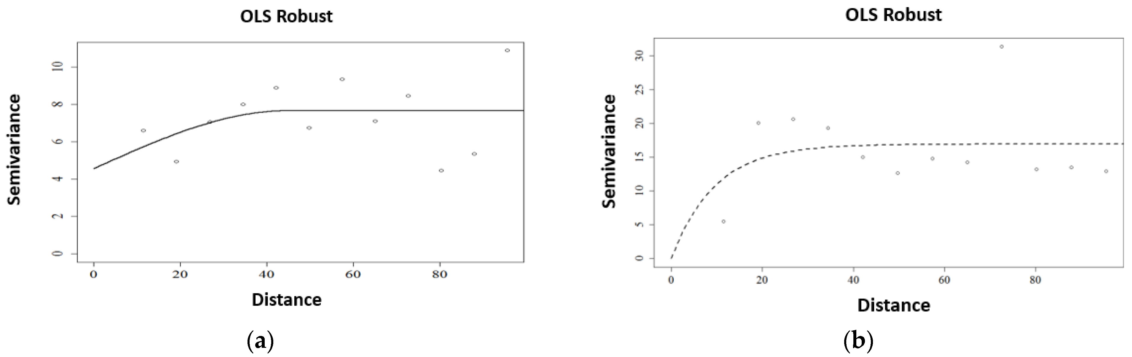
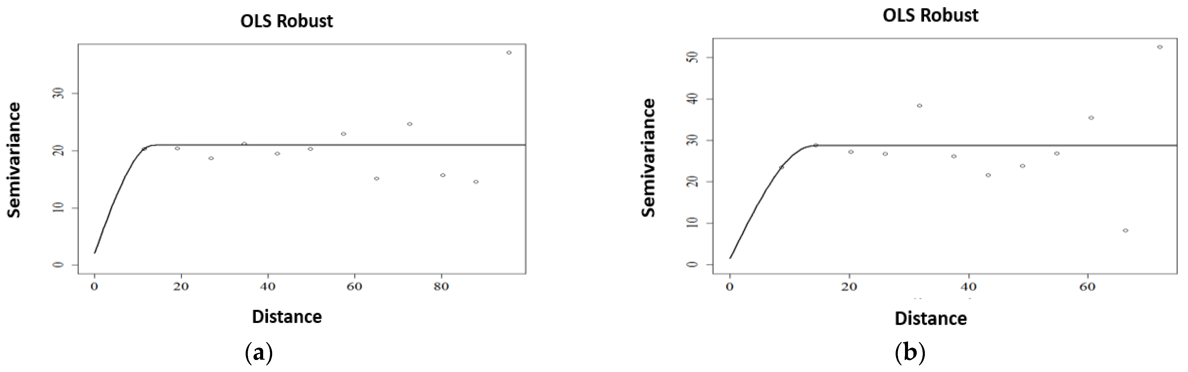
2.4.2. Geostatistical Assessment

Semivariograms were employed to assess the spatial dependence of gravimetric and volumetric moisture. Semivariance was estimated by Equation (4), according to [35]:

$$\widehat{\gamma }\left(h\right)={\displaystyle \frac{1}{2N(h)}}\sum _{i=1}^{Ni=\left(h\right)}\left[Z\right(x_i)-Z(x_i+h)]2$$

(4)

where N (h) is the number of experimental pairs of observations Z(x_i) and Z (x_i + h) separated by a distance h. The semivariogram is represented by the graph as a function of h. By fitting a mathematical model to the calculated values, the coefficients of the theoretical semivariogram model were estimated. These coefficients include the nugget effect (C0), sill (C0 + C), and range (a), as described by [36].

In this study, the ordinary least squares (OLS) method was applied alongside spherical, exponential, and Gaussian models. The selection of the most suitable model was based on the leave-one-out cross-validation (LOO-CV) method, using the lowest mean error (ME) as the criterion. To minimize model bias, the mean error should be as close to zero as possible.

To ensure that the models met cross-validation requirements, the mean error (ME) was calculated following [37], and should be as close to zero as possible. With the adjustment of semivariograms, after detection of the spatial variability, the data were interpolated by ordinary kriging.

The degree of spatial dependence (DSD) of the variables was calculated according to the classification proposed by [38]. This classification indicated strong spatial dependence when the semivariogram’s nugget effect was equal to or less than 25% of the threshold, moderate spatial dependence when it was between 25% and 75%, and weak spatial dependence when it exceeded 75%. Geostatistical analysis was performed using the freely distributed RStudio software version 1.3 [34] and the geoR package [39], while the isoline map was created in QGis software version 3.4.8.

2.5. Image Acquisition and Processing

Images were obtained using an RPA eBee-SQ Sensefly, a fixed-wing model, with an average flight time of 55 min, reaching an average speed of 12 m/s. The aircraft was equipped with a multispectral sensor (Parrot Sequoia model), which includes a high-resolution RGB sensor and four monochromatic sensors for the spectral bands: green (550 ± 40 nm), red (660 ± 40 nm), near-infrared (790 ± 40 nm), and red edge (735 ± 40 nm), with a resolution of 4.71 cm/px. In addition to these sensors, Sequoia has a sensor for luminosity correction, thus obtaining data with radiometric correction. A flight plan was created using a base station and eMotion software 3.5.0 version, provided by the RPA manufacturer. The flight plan presented the following characteristics:

• Focal Length: 3.98 mm.
• Vertical Coverage: 70%.
• Horizontal Cover: 70%.
• Flight Altitude: 50 m.
• Speed: 12 m/s.

The flight was carried out between 11:00 a.m. and 1:00 p.m. to avoid and minimize the influence of lighting geometry (zenithal and azimuthal solar angle).

Before the flight, the multispectral sensor was directed at a calibration reflectance panel, which has a known and uniform reflectance. This procedure allows the system to adjust the measured values, compensating for variations in ambient light and ensuring standardized reflectance readings of the crops. Additionally, the Sequoia features an irradiance light sensor mounted on the top of the drone, which monitors lighting conditions in real time during the flight. This sensor automatically adjusts the captured values to correct variations in sunlight intensity, such as changes in the sun’s angle or the passage of clouds. With the data collected from the calibration panel and the light sensor, the processing software applies corrections to the acquired data, ensuring that the measurements accurately represent the actual conditions of the vegetation and soil, without interference from fluctuations in ambient light.

After completing the flights for each sampling period, the images were processed in Pix4D software 4.5.2 version, generating 5 orthomosaics, 1 being RGB and 4 for the multispectral bands (RED, NIR, RED EDGE, and GREEN).

2.6. Vegetation Indices

The vegetation indices were selected based on the study by [30], which evaluated and identified indices suitable for assessing the spectral response of coffee plants. The vegetation indices calculated for this research are represented in

Table 3. Vegetation indices of images obtained by the multispectral sensor coupled to RPA.

Index	Acronym	Equation	Reference
Normalized Difference Vegetation Index	NDVI	${\displaystyle \frac{NIR-RED}{NIR+RED}}$	[23]
Normalized Difference Water Index	NDWI	${\displaystyle \frac{G-NIR}{G+NIR}}$	[25]
Enhanced Vegetation Index 2	EVI2	$2.5\times {\displaystyle \frac{NIR-RED}{(NIR+2.4\times RED+1)}}$	[40]
Normalized Difference Red Edge	NDRE	${\displaystyle \frac{NIR-REDEdge}{NIR+REDEdge}}$	[41]
Chlorophyll Vegetation Index	CVI	${\displaystyle \frac{NIR}{GREEN}}\times {\displaystyle \frac{RED}{GREEN}}$	[42]
Green Normalized Difference Red Edge	GNDVI	${\displaystyle \frac{NIR-GREEN}{NIR+GREEN}}$	[43]
Canopy Chlorophyll Content Index	CCCI	${\displaystyle \frac{NDRE}{NDVI}}$	[41]
Green Ratio of Vegetation Index	GRVI	${\displaystyle \frac{NIR}{GREEN}}$	[44]
Modified Simple Ratio	MSR	${\displaystyle \frac{\left(\frac{NIR}{RED}\right)-1}{\left(\sqrt{\frac{NIR}{RED}}\right)+1}}$	[45]
Infrared Percentage Vegetation Index	IPVI	${\displaystyle \frac{NIR}{NIR+RED}}$	[46]
Soil-Adjusted Vegetation Index	SAVI	${\displaystyle \frac{(1+L)(NIR-RED)}{L+NIR+RED}}$	[47]
Modified Soil-Adjusted Vegetation Index 2	MSAVI	${\displaystyle \frac{{[2NIR+1-\left({\left(2NIR+1\right)}^2-8\left(NIR-RED\right)\right)}^{0.5}]}{2}}$	[48]
Optimized Soil-Adjusted Vegetation Index	OSAVI	${\displaystyle \frac{(NIR-RED)}{(NIR+RED+0.16)}}$	[49]
Green Chlorophyll Index	CIgreen	$\left({\displaystyle \frac{NIR}{GREEN}}\right)-1$	[24]
Red Edge Chlorophyll Index	CIrededge	$\left({\displaystyle \frac{NIR}{REDEDGE}}\right)-1$	[24]

, containing their respective mathematical formulas, along with references from the authors who developed them.

2.7. Correlation Analysis

To determine the relationship between the calculated vegetation indices and the gravimetric and volumetric moisture attributes, a correlation analysis was performed. Basically, correlation analysis summarizes the degree of relationship that exists between two or more variables (x and y, for example).

For the correlation analysis, a shapefile was created containing 30 polygons, each with a diameter of 0.20 m (20 cm). These polygons were precisely positioned at the center of the canopy of each sampled plant. This approach aimed to ensure that the calculations considered only the plant’s foliage area, minimizing interference from other elements such as bare soil and shadows.

Vegetation index values were extracted using the zonal statistics tool in QGIS software. This tool calculates descriptive statistics for the pixel values contained within each defined polygon. In this study, the average pixel value within each polygon corresponding to a sampled plant was computed.

As a result, for each vegetation index calculated, 30 average values were obtained, corresponding to the 30 georeferenced sampled plants. This procedure guaranteed that the values utilized in the correlation analysis accurately reflected the actual canopy conditions of each plant, minimizing the influence of external variations.

The average values of each vegetation index, along with the gravimetric and volumetric moisture values, were exported to a table for calculating the Pearson correlation coefficient (R), as expressed in Equation (5). The R value consistently ranged from −1 to 1. The interpretation of the coefficient (R) followed the criteria established in the study by [50].

$$R={\displaystyle \frac{n{\sum }_{i=1}^n{x}_i{y}_i-{\sum }_{i=1}^n{x}_i{\sum }_{i=1}^n{y}_i}{\sqrt{n{\sum }_{i=1}^n{x}_{i}2-({\sum }_{i=1}^n{x}_i)2}\sqrt{n{\sum }_{i=1}^n{y}_{i}2({\sum }_{i=1}^n{y}_i)2}}}$$

(5)

3. Results

3.1. Statistical Evaluation

3.1.1. Statistical Summary

Table 4. Gravimetric moisture (Gm) and volumetric moisture (Vm) in dry season (Dry) and rainy season (Rainy).

Season	Variables (%)	Min	Max	Md	Mean	Var	SD	CV (%)
Dry	Gm (0–10 cm)	12.50	20.64	17.67	17.22	3.65	1.91	0.11
Dry	Gm (10–20 cm)	11.75	19.33	17.93	17.61	2.63	1.62	0.09
Rainy	Gm (0–10 cm)	19.52	29.54	25.52	24.83	6.00	2.45	0.09
Rainy	Gm (10–20 cm)	18.48	27.97	25.69	25.26	4.94	2.22	0.08
Dry	Vm (0–10 cm)	18.92	31.19	23.06	23.57	7.34	2.68	0.11
Dry	Vm (10–20 cm)	15.36	36.19	23.23	22.74	13.93	3.73	0.16
Rainy	Vm (0–10 cm)	26.24	45.45	34.39	35.02	8.08	2.84	0.07
Rainy	Vm (10–20 cm)	22.79	48.85	34.68	33.87	25.37	5.03	0.14

Min—minimum value; Max—maximum value; Md—median; Mean—mean; Var—variance; SD—standard deviation; CV—coefficient of variation (%).

compares the gravimetric moisture (Gm) and volumetric moisture (Vm) of the soil at different depths (0–10 cm and 10–20 cm) during the dry and rainy seasons.

The results indicate that the moisture content for both Gm and Vm was significantly higher during the rainy season compared with the dry season. Soil moisture tended to be slightly lower at a depth of 10–20 cm, where the average values were 15.36% for volumetric moisture and 18.48% for gravimetric moisture, compared with the 0–10 cm layer, which presented 18.92% and 12.50%, respectively. This difference was more evident during the dry season. The variability of volumetric moisture (Vm) and gravimetric moisture (Gm) was considered low (<12%) under all conditions, except for Vm during the rainy season, which was classified as moderate.

The monthly accumulated precipitation data indicate a significant difference between the analyzed periods. During the dry season in August 2020, precipitation was only 17.6 mm, whereas in the rainy season of January 2021, it reached 270.6 mm. Consequently, soil water availability was impacted, reflecting in the gravimetric Gm and volumetric Vm moisture values. The water balance also illustrates this difference, with a water deficit of 94.1 mm in the dry season, while, in the rainy season, there was a surplus of 212.9 mm, indicating a greater availability of water in the soil for plant absorption.

The study area’s altitude ranged from 917 to 935 m, with an altimetric difference of 18 m. The soil texture was classified as clayey 36 to 38 percent clay, 32 to 33 percent silt, and 29 to 32 percent sand, which provides a high-water retention capacity. Clayey soils, such as those observed in this area, tend to retain more water, especially during rainy seasons, reducing surface runoff and increasing moisture storage. However, this same characteristic can lead to slower drainage, and under excess water conditions, it may hinder water absorption by plants due to low porosity.

Based on soil water storage through the water balance shown in Figure 4, it can be stated that, during the dry season, volumetric moisture was closer to water deficit zones, making absorption by plants more difficult. In the rainy season, the higher moisture values remained close to or above the maximum storage capacity, ensuring greater water availability for the roots.

The results corroborate the statements of [51], who highlighted the influence of climatic factors, especially precipitation and temperature, on the phenological phases of coffee plants. The variation in soil moisture throughout the year can directly impact coffee productivity and quality, as periods of water deficiency may compromise vegetative growth and fruiting.

Additionally, the analyzed data align with the observations of [52], who emphasized the need for adequate moisture between October and May to ensure fruit growth and filling, while a dry season after May favors uniform grain ripening and flowering induction. The water balance evidenced in this study reinforces this necessity, demonstrating that water deficiency during the dry season can hinder crop development, while the greater availability of water in the rainy season is essential for the coffee plant’s productive cycle.

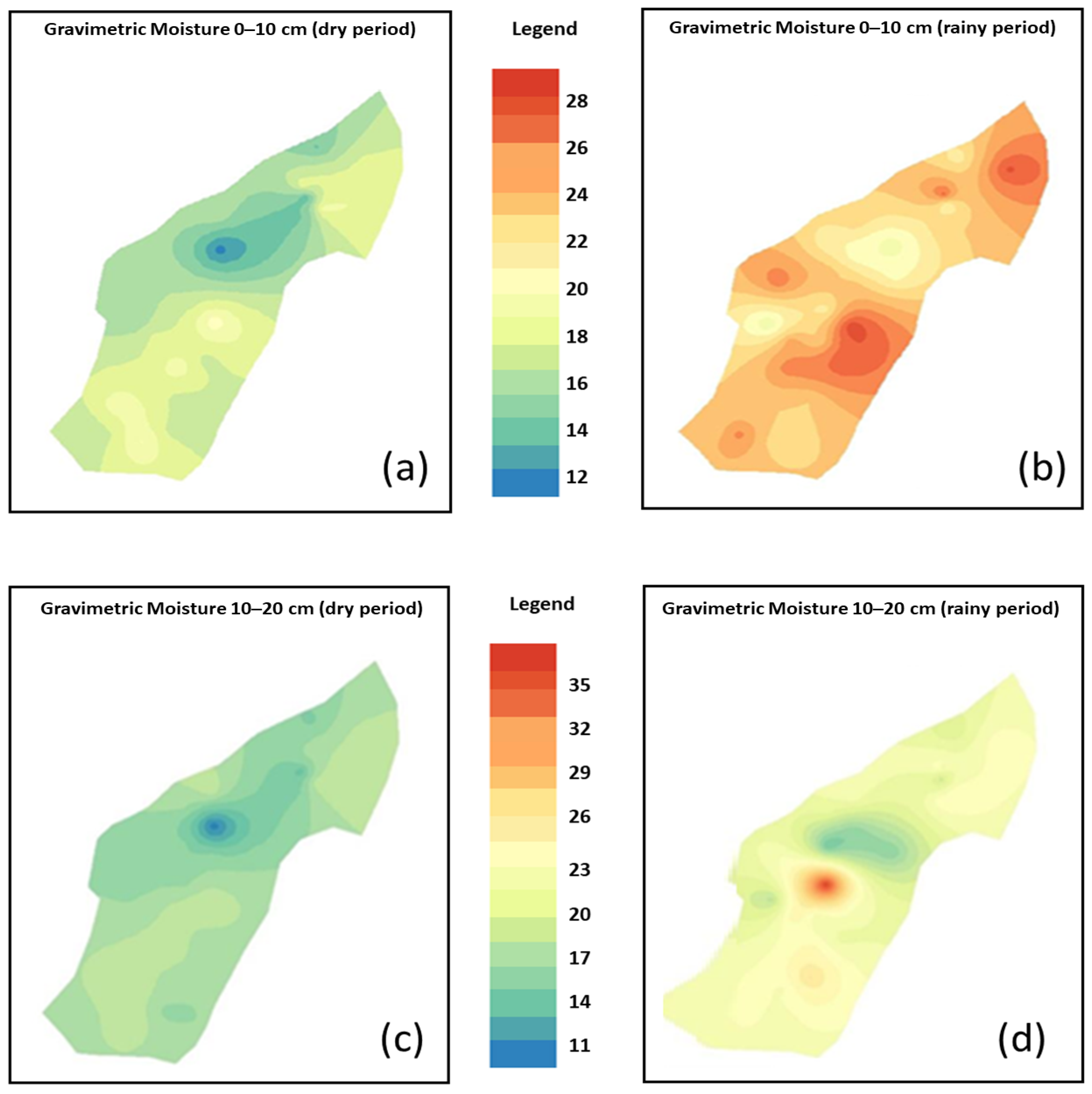
3.1.2. Geostatistical Analysis

The semivariogram adjustment parameters—nugget effect (C0), contribution (C1), threshold (C0 + C1), and range (A)—were determined using the ordinary least squares (OLS) method with spherical and exponential models. The values for the degree of spatial dependence (DSD) and mean error (ME) are presented in

Table 5. Parameters used in modeling the geostatistical semivariogram of gravimetric moisture (Gm) and volumetric moisture (Vm) during the dry season (Dry) and the rainy season (Rainy).

Season	Variable	Mod.	C0	C1	C0 + C1	A (m)	DSD		ME
Dry	Gm (0–10 cm)	Sph	0.01	3.50	3.51	70.00	0.28	strong	−0.00
	Gm (10–20 cm)	Sph	0.10	2.50	2.60	40.00	3.84	strong	0.01
	Vm (0–10 cm)	Exp	0.25	3.80	4.05	35.00	6.17	strong	−0.02
	Vm (10–20 cm)	Exp	0.01	4.00	4.01	50.00	0.24	strong	0.00
Rainy	Gm (0–10 cm)	Sph	0.00	8.00	8.00	45.00	0.00	strong	0.00
	Gm (10–20 cm)	Exp	0.00	15.00	15.10	40.00	0.66	strong	0.00
	Vm (0–10 cm)	Sph	0.01	22.00	22.01	20.00	0.04	strong	−0.02
	Vm (0–10 cm)	Sph	0.01	28	28.01	20.00	0.00	strong	0.07

nugget effect: C0; contribution: C1; sill: C0 + C1; range: A; degree of spatial dependence (DSD); mean error (ME); model used (Mod); spherical (Sph); exponential (Exp).

.

Geostatistical analysis of soil moisture, both gravimetric (Gm) and volumetric (Vm), was conducted using spherical (Sph) and exponential (Exp) models for different depths (0–10 cm and 10–20 cm) and seasons (dry and rainy).

The results revealed that all variables exhibited strong spatial dependence (SSD), indicating that soil moisture follows a defined spatial pattern. The range varied from 45 to 20 m in the rainy season and from 70 to 35 m in the dry season.

The mean error (ME) was low for all variables, confirming the accuracy of the geostatistical models applied. Variations in the semivariogram parameters were observed between the dry and rainy seasons, reflecting changes in the spatial structure of soil moisture throughout the year.

Analysis of the four semivariograms (Figure 5 and Figure 6) provided an overview of the spatial dependence of soil moisture (gravimetric and volumetric) at both depths (0–10 cm and 10–20 cm) during the dry season.

All four graphs indicate spatial dependence, with semivariance increasing with distance (20–40 m) until reaching a sill.

Figure 7a–d and Figure 8a–d represent kriging maps of soil gravimetric moisture in percentage (%) at depths of 0–10 cm and 10–20 cm during the dry and rainy seasons, respectively. These maps were generated to visualize the spatial distribution of soil moisture in the study area.

The values in Figure 7 and Figure 8 exhibit high variability. This variation highlights how relying solely on the means of field observations can lead to management errors, as discussed in studies by [51,52]. These findings underscore the significance of precision agriculture (PA) in coffee production management and highlight the relevance of statistical tools that incorporate spatial relationships.

In Figure 8c, Vm 10–20 cm (dry season) presents a relatively homogeneous spatial distribution of soil moisture in the study area. A slight variation is observed, with some areas appearing wetter (18% to 23%) and others drier (27%). The color gradient indicates that cooler colors (green shades) represent areas with lower moisture, while warmer colors (yellow shades) indicate areas with higher moisture.

In Figure 8d, Vm 10–20 cm (rainy season), the map indicates greater variability in soil moisture compared with the dry season. High-moisture areas are depicted in warm colors, whereas low-moisture areas appear in cool colors. A more distinct moisture distribution pattern is evident, with high-moisture zones concentrated in specific regions of the map. This suggests that rainfall may have contributed to a heterogeneous distribution of moisture across the study area.

3.2. Statistical Correlation Between Vegetation Indices and Soil Moisture

To assess the potential of high-resolution images for detecting the water status of coffee trees, correlation analysis was conducted between field-collected soil moisture data and vegetation indices (Table 3).

Table 6. Correlation analysis between vegetation indices and soil gravimetric moisture (Gm) and volumetric moisture (Vm) in dry season (Dry) and rainy season (Rainy).

Index	Gm (0–10 cm)		Gm (10–20 cm)		Vm (0–10 cm)		Vm (10–20 cm)
	Dry	Rainy	Dry	Rainy	Dry	Rainy	Dry	Rainy
RED	0.3005 ns	0.2767 ns	0.1235 ns	0.2781 ns	0.4637 *	0.4163 *	0.2668 ns	0.4368 *
NIR	0.1991 ns	0.0185 ns	0.0938 ns	0.0110 ns	0.2213 ns	0.1155 ns	0.2210 ns	0.1020 ns
RED EDGE	0.1782 ns	0.0878 ns	0.0355 ns	0.1732 ns	0.2608 ns	0.0506 ns	0.2289 ns	0.0197 ns
GREEN	0.2840 ns	0.0618 ns	0.1093 ns	0.3141 ns	0.5157 *	0.1692 ns	0.3601 ns	0.2597 ns
NDVI	0.1328 ns	0.1791 ns	0.0463 ns	0.1604 ns	0.2421 ns	0.3275 ns	0.0871 ns	0.3329 ns
NDWI	0.0129 ns	0.0841 ns	0.0299 ns	0.2558 ns	0.1079 ns	0.2815 ns	0.0011 ns	0.3418 ns
EVI2	0.0627 ns	0.0584 ns	0.0375 ns	0.0330 ns	0.0177 ns	0.1738 ns	0.0950 ns	0.1652 ns
NDRE	0.1202 ns	0.0853 ns	0.1854 ns	0.2312 ns	0.0156 ns	0.1809 ns	0.0786 ns	0.2458 ns
CVI	0.4363 *	0.0277 ns	0.2487 ns	0.2798 ns	0.3791 *	0.1283 ns	0.2602 ns	0.2195 ns
GNDVI	0.0129 ns	0.0841 ns	0.0299 ns	0.2558 ns	0.1079 ns	0.2815 ns	0.0011 ns	0.3418 ns
CCCI	0.0431 ns	0.0277 ns	0.1035 ns	0.0325 ns	0.0881 ns	0.1454 ns	0.0302 ns	0.2664 ns
GVI	0.0409 ns	0.1141 ns	0.0287 ns	0.2642 ns	0.0833 ns	0.3033 ns	0.0129 ns	0.3587 ns
MSR	0.1328 ns	0.1791 ns	0.0463 ns	0.1604 ns	0.2421 ns	0.3275 ns	0.0871 ns	0.3329 ns
IPVI	0.1328 ns	0.1791 ns	0.0463 ns	0.1604 ns	0.2421 ns	0.3275 ns	0.0871 ns	0.3329 ns
SAVI	0.0827 ns	0.0655 ns	0.0480 ns	0.0411 ns	0.0457 ns	0.1848 ns	0.1171 ns	0.1774 ns
MSAVI	0.0158 ns	0.0542 ns	0.0200 ns	0.0301 ns	0.0490 ns	0.1696 ns	0.0536 ns	0.1613 ns
OSAVI	0.0076 ns	0.1002 ns	0.0098 ns	0.0778 ns	0.0799 ns	0.2321 ns	0.0331 ns	0.2287 ns
CIgreen	0.0409 ns	0.1141 ns	0.0287 ns	0.2642 ns	0.0833 ns	0.3033 ns	0.0129 ns	0.3587 ns
CIrededge	0.1360 ns	0.0876 ns	0.1941 ns	0.2377 ns	0.0005 ns	0.1751 ns	0.0908 ns	0.2424 ns

ns—not significant, * = significant at 5%.

presents the R values (Pearson correlation coefficients) for the studied variables, spectral bands, and vegetation indices. An F-test was performed to evaluate the significance of the correlations at the 0.05 (5%) significance level.

The RED spectral band (dry and rainy seasons) and the GREEN spectral band (rainy season), along with the chlorophyll vegetation index (CVI) (dry and rainy seasons), exhibited significant correlations at the 5% significance level, according to Pearson’s correlation analysis (Figure 9, Figure 10 and Figure 11). The CVI exhibited the strongest statistically significant positive correlation with Gm (0–10 cm) (r = 0.4363).

The GREEN index exhibited the strongest significant positive correlation with Vm (0–10 cm) (r = 0.5157). The RED index exhibited the strongest significant positive correlation with Vm (10–20 cm) (r = 0.4368).

Figure 9, Figure 10 and Figure 11 illustrate the spectral analysis across different seasons. Figure 9 depicts the RED band for the dry season (a) and the rainy season (b), Figure 10 represents the GREEN band for both seasons, and Figure 11 illustrates the CVI vegetation index for the dry season (a) and the rainy season (b).

The RED band exhibited values ranging from 0.01 to 0.33, with no noticeable visual differences between the two periods (Table 1). The GREEN spectral band ranged from 0.01 to 0.24, with predominant values between 0.01 and 0.08 during the dry season and between 0.08 and 0.16 during the rainy season. The CVI vegetation index displayed distinct visual differences between the two periods, ranging from 5.76 to 8.17 in the dry season and from 0.94 to 3.35 in the rainy season.

4. Discussion

4.1. Descriptive Statistics

During the dry season, the variables Gm (10–20 cm) and Vm (0–10 cm and 10–20 cm) exhibited CV values below 10%. The CV value for Gm at 0–10 cm was 11%, indicating moderate variability. In the rainy season, only Vm (0–10 cm) exhibited low heterogeneity (CV < 10%), while the other variables presented moderate heterogeneity (10% < CV < 20%).

The lowest gravimetric and volumetric moisture values during the dry season were recorded at depths of 10–20 cm, at 11.75% and 18.48%, respectively. A similar pattern was observed during the rainy season, with the lowest gravimetric and volumetric moisture values recorded at depths of 10–20 cm (15.36% and 22.79%). The highest moisture values for both the dry and rainy seasons were recorded at depths of 0–10 cm for both gravimetric and volumetric measurements.

The gravimetric moisture levels observed in coffee cultivation soils in this study were consistent with those reported by [53], who recorded a mean value of 17.82%, and [54], who reported values of 18.20% at a depth of 0–20 cm and 20.00% at 20–40 cm. Another similarity between this study and [54] is that the gravimetric moisture values did not vary significantly with sampling depth.

The mean gravimetric moisture values recorded were 17.67% for samples collected at a depth of 0–10 cm and 17.93% for samples collected at a depth of 10–20 cm in the dry season. In the rainy season, the values were 23.06% and 23.23% for samples collected at depths of 0–10 cm and 10–20 cm, respectively. The mean volumetric moisture values recorded were 24.83% and 25.26% at depths of 0–10 cm and 10–20 cm, respectively, during the dry season. For the rainy season, the values were 35.02% for the 0–10 cm sampling depth and 33.87% for the 0–20 cm depth.

Ref. [55] assessed soil volumetric moisture at three depths (0–5 cm, 5–10 cm, and 10–20 cm), reporting values of 45.00%, 41.00%, and 38.00%, respectively. The volumetric moisture at a depth of 0–10 cm in this study (35.02%) closely matched the value reported by [55], who recorded 38.00% at a depth of 10–20 cm. Another common finding was the decline in volumetric moisture as sampling depth increased.

Refs. [51,53] analyzed the physical attributes of a coffee plantation located in the municipality of Três Pontas. Both studies determined gravimetric moisture values from samples collected at six depth layers within a 0–60 cm soil profile. Ref. [51] reported an average moisture content of 22.33%, while [53] reported an average moisture range of 20.57% to 24.58%. These authors examined five coffee strains of different heights. The average soil moisture values reported by these authors closely resembled those observed in this study. Although the sampling depth differed, the crop and the region studied remained the same.

Gravimetric and volumetric moisture levels increased during the dry season (August 2020) and the wet season (January 2021). One of the main factors influencing this condition was rainfall during these periods. According to the precipitation data in Table 1, the last recorded rainfall before data collection in August 2020 occurred 74 days earlier (20 mm on 31 May 2020, which was likely associated with a period of water scarcity for the crop. In contrast, a total of 115 mm of rainfall was recorded seven days before the second collection in January 2021 (Table 1), representing a precipitation volume six times greater than that observed prior to data collection in the dry season.

Analyzing the mean, maximum, minimum, and CV values presented in Table 5 revealed variations between measurements. However, simply knowing these values was insufficient to fully express variable variability. Therefore, a geostatistical analysis was necessary to evaluate the spatial distribution of the attributes assessed in this study. In addition to the geostatistical assessment, thematic maps were generated to facilitate the visual interpretation of the spatial distribution of attributes within the study area.

4.2. Climatic Conditions, Water Balance, Altitude, and Soil Properties

Climatic data further highlighted the impact of seasonal variations on soil moisture. The accumulated monthly precipitation data revealed a significant difference between the analyzed periods. In August 2020 (dry season), precipitation totaled only 17.6 mm, whereas, in January 2021 (rainy season), it reached 270.6 mm. Consequently, soil water availability was affected, reflected in the gravimetric (Gm) and volumetric (Vm) moisture values. The water balance further illustrated this contrast, with a water deficit of 94.1 mm during the dry season, while, in the rainy season, there was a surplus of 212.9 mm, indicating greater water availability in the soil for plant absorption.

Temperature and relative humidity also played significant roles in soil moisture variation. During the dry season, the monthly mean temperature was 18.3 °C, with a lower relative humidity of 59.3%. The reduced atmospheric moisture content, combined with a higher potential evapotranspiration (PET) of 53.8 mm, contributed to soil water loss, exacerbating the water deficit. In contrast, the rainy season recorded a higher monthly mean temperature of 23.0 °C but with an increased relative humidity of 70.9%. The elevated humidity reduced evaporative demand, preserving soil moisture. Additionally, the lower PET value of 110.0 mm in the rainy season, combined with high precipitation, resulted in greater soil moisture retention and water surplus.

Wind speed also affected soil moisture conditions. During the dry season, the average wind speed was 2.0 m/s, slightly higher than the 1.7 m/s recorded in the rainy season. Stronger winds can accelerate soil moisture loss by increasing evapotranspiration, further exacerbating water scarcity in the dry season. Conversely, lower wind speeds in the rainy season contributed to reduced evaporation rates, promoting moisture retention.

The study area’s altitude ranged from 917 to 935 m, with an elevation difference of 18 m. The soil texture was classified as clayey (36–38% clay, 32–33% silt, and 29–32% sand), providing high water retention capacity. Clayey soils, such as those in this area, tend to retain more water, especially during rainy seasons, reducing surface runoff and increasing moisture storage. However, this characteristic can also lead to slower drainage, and, under excess water conditions, it may hinder plant water absorption due to low porosity.

Based on the soil water storage derived from the water balance, it can be concluded that, during the dry season, volumetric moisture was closer to water deficit zones, making plant absorption more difficult. In the rainy season, higher moisture values remained near or above the maximum storage capacity, ensuring greater water availability for the roots.

The results corroborated the findings of [56], who highlighted the impact of climatic factors, particularly precipitation and temperature, on the phenological stages of coffee plants. Variations in soil moisture throughout the year can directly impact coffee productivity and quality, as periods of water deficiency may compromise vegetative growth and fruit development.

Furthermore, the analyzed data were consistent with the observations of [57], who stressed the importance of adequate moisture between October and May to ensure fruit growth and filling, while a dry season after May promotes uniform grain ripening and flowering induction. The water balance observed in this study reinforced this requirement, demonstrating that water deficiency during the dry season can hinder crop development, whereas greater water availability in the rainy season is essential for the coffee plant’s productive cycle.

4.3. Geostatistical Analysis

Ref. [58] reported that variables related to water retention exhibited greater continuity and spatial dependence. Conversely, [59] indicated that soil moisture varied significantly within the 0–20 cm sampling interval. These findings were validated in this study, as soil moisture measured at a depth of 0–20 cm demonstrated spatial dependence, as evidenced by the geostatistical data (Table 6 and Figure 3 and Figure 4).

The spherical and exponential models were suitable for data modeling, as the mean error (ME) values were very close to zero, thus meeting the cross-validation criteria. The attribute Vm 10–20 cm had the highest mean error value (0.0661) during the rainy season, while the lowest mean error value was observed for Gm 10–20 cm (ME = 0.0010), also during the rainy season.

In this study, all evaluated variables exhibited a strong degree of spatial dependence (DSD). A similar pattern was observed by [51,55], who analyzed the spatial variability of soil physical attributes in coffee cultivation areas and identified a strong degree of spatial dependence (DSD) for soil moisture.

Ref. [55] reported that, in geostatistical modeling for soil science studies, the spherical model is the most frequently applied. However, semivariogram adjustments related to soil properties are often observed for both spherical and exponential models.

When analyzing the range values during the dry season, it was observed that the shallower the sampling depth (0–10 cm), the greater the range for gravimetric and volumetric moisture values. In contrast, this phenomenon was not observed in the rainy season, that is, despite variations in sampling depth, the range values remained equal (Vm) or very close (Gm: A = 45 and Gm: A = 40).

The kriging map indicated that gravimetric moisture at a depth of 0–10 cm in the dry season (Figure 7a) ranged from 12% to 20%, with predominant values between 16% and 20%. In the rainy season, gravimetric moisture at the same depth (Figure 7b) ranged from 20% to 28%. At a depth of 10–20 cm (Figure 7c), gravimetric moisture varied from 12% to 18%, with predominant values between 12% and 14%. The kriging map of Vm (10–20 cm) in the rainy season (Figure 7d) revealed a moisture variation between 20% and 35%, with values above 25% being predominant.

The kriging maps for volumetric moisture at a depth of 0–10 cm (Figure 8a,b) predominantly varied from 20% to 27% in the dry season and from 30% to 42% in the rainy season. The spatial map of volumetric moisture at a depth of 10–20 cm (Figure 8c,d) indicated a predominant range of 23% to 27% in the dry season and 32% to 36% in the rainy season.

The maps demonstrated that locations with higher and lower soil moisture concentrations remained consistent between the two periods, though a general increasing trend was observed. This pattern was attributed to the sampling times, which were conducted in two distinct climatic seasons (dry and rainy).

4.4. Analysis of Correlation Between Field Data and Vegetation Indices

The correlations described in Table 5 do not imply causality, as the observed relationships may be influenced by other factors not considered in this study. Vegetation indices are affected by multiple variables, including vegetation type, soil cover, and atmospheric conditions, all of which can impact their relationship with soil moisture.

Figure 9a illustrates the reflectance of the red band during the dry season, where lighter tones indicate exposed soil or sparse vegetation, while darker tones suggest denser vegetation cover or higher soil moisture. In Figure 9b, representing the rainy season, an overall reduction in reflectance was observed, indicating increased vegetation density or soil moisture.

According to [22], vegetation absorbs most of the radiation in the visible spectrum, with absorption peaks in the blue and red regions due to chlorophyll activity. Greater vegetation activity results in higher absorption in the red band, leading to lower reflectance. Seasonal variations in reflectance reflect changes in chlorophyll activity influenced by water availability, while spatial differences within each season may be associated with leaf cellular structure, soil texture, and topography.

Ref. [60] investigated the water conditions of a coffee crop by evaluating potential correlations between leaf water potential and multispectral bands, along with vegetation indices derived from high-resolution images captured by RPA. The authors identified a significant correlation of 39.93% between the red spectral band and leaf water potential.

Ref. [29] examined the correlation between chlorophyll and NDVI obtained using passive and active sensors. The study was conducted in a coffee plantation, where the authors established sampling grids of 30, 60, 90, and 120 points to assess the correlation between attributes. The results indicated a significant correlation between NDVI obtained via active sensors and chlorophyll (31%) for the 90-point grid and (48%) for the 120-point grid. NDVI continues to be one of the most extensively utilized indices due to its integration of near-infrared and red spectral bands [22].

Figure 10 illustrates the reflectance of the green band during the rainy season, following the same pattern as the red band. Lighter tones indicate higher reflectance, while darker tones represent lower reflectance. Figure 11a displays the CVI index during the dry season, where lower values indicate reduced chlorophyll content and possible plant stress, whereas higher values suggest greater vigor. In Figure 11b, corresponding to the rainy season, a general increase in CVI is observed, represented by redder tones, indicating higher chlorophyll content and greater plant vigor. These Figures highlight the seasonal variations in spectral reflectance and the CVI vegetation index. During the rainy season, lower reflectance is observed in both the red and green bands, accompanied by an increase in CVI, suggesting greater vegetation cover, higher chlorophyll content, and potentially higher soil moisture.

The green coloration of plants results from chlorophylls preferentially absorbing light in the blue and red regions of the electromagnetic spectrum while reflecting light in the green region. The more active and healthier the vegetation, the greater the absorption of red light by chlorophyll, consequently leading to lower reflectance in this spectral range. Conversely, in stressed plants or those with lower chlorophyll content, red light absorption decreases, resulting in higher reflectance. This characteristic forms the basis for using vegetation indices, such as CVI, which assess vegetation health by comparing red light absorption with reflectance in the near-infrared region.

Studies by [42] indicate that CVI exhibits high sensitivity to leaf chlorophyll concentration. Moreover, even in soils with significant reflectance variability due to moisture, CVI maintains a stable linear relationship with chlorophyll concentration, particularly under extreme conditions of completely dry or wet soil. This result highlights the robustness of the index in adapting to soil moisture variations.

The aforementioned authors emphasize in their studies the applications of RPA in coffee farming, along with the evaluation of possible correlations between coffee tree attributes and vegetation indices. However, to date, no studies have been identified that assess the water conditions of coffee trees using high-resolution images while incorporating soil moisture variability analysis.

5. Conclusions

Gravimetric and volumetric moisture data collected at different depths and during different periods (dry and rainy seasons) served as a basis for evaluating the spatial variability of these attributes through geostatistical analysis. By adjusting semivariograms, a mathematical function was fitted to express the spatial dependence structure of soil moisture. Additionally, kriging interpolation enabled the estimation of this attribute’s values in unsampled locations.

Spatial variability in the studied variables was assessed by calculating the coefficient of variation, which indicated strong spatial dependence for all evaluated variables. The semivariograms were best fitted to the spherical and exponential models. The kriging maps illustrate the spatial distribution of the studied variables, allowing the identification of areas with higher and lower intensities for each variable.

Conversely, vegetation indices revealed the extent to which a crop’s reflectance values fluctuate between different periods (i.e., dry and rainy seasons). These methods allowed the evaluation of multiple parameters, including plant health, chlorophyll content, and leaf water content. Therefore, correlation and regression analyses were conducted to assess whether soil moisture was correlated with vegetation indices. The results indicated that the RED and GREEN spectral bands, along with the CVI index, were significantly correlated with soil moisture.

The application of geostatistical tools and vegetation indices derived from high-resolution images proved to be effective in this study. However, future research could enhance the efficiency of these tools for monitoring and detecting water variability in coffee plantations, providing valuable support for producers in making informed management decisions.

References

1. Esposito, F.; Fasano, E.; De Vivo, A.; Velotto, S.; Sarghini, F.; Cirillo, T. Processing effects on acrylamide content in roasted coffee production. Food Chem. 2020, 319, 126550. [Google Scholar] [PubMed]
2. CONAB-Companhia Nacional de Abastecimento. Acompanhamento da Safra Brasileira de Café, Brasília, DF, v.11, n. 4, Quarto Levantamento, Janeiro 2025. Available online: https://www.conab.gov.br/info-agro/safras/cafe/boletim-da-safra-de-cafe (accessed on 3 March 2025).
3. Aparecido, L.E.O.; Rolim, G.S.; Souza, P.S. Sensitivity of newly transplanted coffee plants to climatic conditions at altitudes of Minas Gerais, Brazil. Aust. J. Crop Sci. 2015, 9, 160–167. [Google Scholar]
4. de Sá Júnior, A.; de Carvalho, L.G.; Da Silva, F.F.; de Carvalho Alves, M. Application of the Köppen classification for climatic zoning in the state of Minas Gerais, Brazil. Theor. Appl. Climatol. 2012, 108, 1–7. [Google Scholar]
5. Camargo, M.B.P. The impact of climatic variability and climate change on arabic coffee crop in Brazil. Bragantia 2010, 69, 239–247. [Google Scholar]
6. International Coffee Organization (ICO). Coffee Report and Outlook April 2023. 2023. Available online: https://icocoffee.org/documents/cy2022-23/Coffee_Report_and_Outlook_April_2023_-_ICO.pdf (accessed on 14 October 2024).
7. Lopes, C.C.; Valente, G.F.; de Cinque Mariano, D.; Okumura, R.S.; de Jesus Matos Viégas, I.; Ferraz, G.A.e.S.; Ferraz, P.F.P.; Dos Santos, S.A. Spatial Variability of Soil Resistance to Penetration in Fruit Cultivation in Eastern Amazonia. AgriEngineering 2023, 5, 1302–1313. [Google Scholar] [CrossRef]
8. Vicente, M.R.; Mantovani, E.C.; Fernandes, A.L.T.; Neves, J. Efeitos da irrigação na produção e no desenvolvimento do cafeeiro na região oeste da Bahia. Coffee Sci. 2017, 12, 544–551. [Google Scholar] [CrossRef]
9. Rezende, F.C.; Oliveira, S.D.R.; Faria, M.A.D.; Arantes, K.R. Características produtivas do cafeeiro (Coffea arabica L. cv.,Topázio MG-1190), recepado e irrigado po gotejamento. Coffee Sci. 2006, 1, 103–110. [Google Scholar]
10. Mantovani, E.C.; Bernardo, S.; Palaretti, L.F. Irrigação: Princípios e Métodos; Editora UFV: Viçosa, MG, Brazil, 2009; 355p. [Google Scholar]
11. Ávila, L.F.; Mello, C.R.d; Silva, A.M.d. Continuity and spatial distribution of soil moisture in the Serra da Mantiqueira watershed. Rev. Bras. Eng. Agríc. Ambient. 2010, 14, 1257–1266. (In Portuguese) [Google Scholar]
12. Zucco, G.; Brocca, L.; Moramarco, T.; Morbidelli, R. Influence of land use on soil moisture spatial–temporal variability and monitoring. J. Hydrol. 2014, 516, 193–199. [Google Scholar]
13. Zhang, M.; Li, M.; Wang, W.; Liu, C.; Gao, H. Temporal and spatial variability of soil moisture based on WSN. Math. Comput. Model. 2013, 58, 826–833. [Google Scholar] [CrossRef]
14. Kim, Y.; Evans, R.G.; Iversen, W.M. Remote sensing and control of an irrigation system using a distributed wireless sensor network. IEEE Trans. Instrum. Meas. 2008, 57, 1379–1387. [Google Scholar]
15. Santos, S.A.; Ferraz, G.A.S.; Figueiredo, V.C.; Volpato, M.M.L.; Matos, C.S.M.; Pereira, A.B.; Conti, L.; Bambi, G.; Marin, D.B. Spatial and temporal variability of productivity of coffee plants grown in an experimental field located in Três Pontas, Brazil. Agron. Res. 2023, 21, 1567–1580. [Google Scholar] [CrossRef]
16. de Assis Silva, S.; de Souza Lima, J.S.; de Souza, G.S. Estudo da fertilidade de um Latossolo Vermelho-Amarelo húmico sob cultivo de café arábica por meio de geoestatística. Rev. Ceres 2010, 57, 560–567. [Google Scholar]
17. Colomina, I.; Molina, P. Unmanned aerial systems for photogrammetry and remote sensing: A review. ISPRS J. Photogramm. Remote Sens. 2014, 92, 79–97. [Google Scholar]
18. Schirrmann, M.; Giebel, A.; Gleiniger, F.; Pflanz, M.; Lentschke, J.; Dammer, K.-H. Monitoring agronomic parameters of winter wheat crops with low-cost UAV imagery. Remote Sens. 2016, 8, 706. [Google Scholar] [CrossRef]
19. Padolfi, A.S.; Ramaldes, G.P.; dos Santos, O.L. Vegetation Index Analysis Using Images Obtained By Vant. Rev. Cient. Faesa 2018, 14, 142–162. (In Portuguese) [Google Scholar]
20. Pezzopane, J.R.M.; Bernardi, A.C.C.; Bosi, C.; Crippa, P.H.; Santos, P.M.; Nardachione, E.C. Assessment of Piatã palisadegrass forage mass in integrated livestock production systems using a proximal canopy reflectance sensor. Eur. J. Agron. 2019, 103, 130–139. [Google Scholar]
21. Shiratsuchi, L.S.; Brandao, Z.N.; Vicente, L.E.; Victoria, D.C.; Ducati, J.R.; Oliveira, R.P.; Vilela, M.F. Remote Sensing: Basic concepts and applications in Precision Agriculture. In Precision Agriculture: Results from a New Perspective; Bernardi, A.C.C., Naime, J.M., Resende, A.V., Bassoi, L.H., Inamasu, R.Y., Eds.; Embrapa: Brasília, Brazil, 2014; pp. 58–73. [Google Scholar]
22. Queiroz, D.M.; Valente, D.S.M.; Pinto, F.A.C.; Borém, A. Agricultura Digital, 2nd ed.; Oficina de Textos: São Paulo, Brazil, 2022. [Google Scholar]
23. Rouse, J.; Haas, R.; Schell, J.; Deering, D. Monitoring Vegetation Systems in the Great Plains with ERTS. Proc. Earth Resour. Technol. Satell. Symp. 1973, 1, 309–317. [Google Scholar]
24. Gitelson, A.A.; Viña, A.; Ciganda, V.; Rundquist, D.C.; Arkebauer, T.J. Remote estimation of canopy chlorophyll content in crops. Geophys. Res. Lett. 2005, 32, 1–4. [Google Scholar] [CrossRef]
25. McFeeters, S.K. The use of the Normalized Difference Water Index (NDWI) in the delineation of open water features. Int. J. Remote Sens. 1996, 17, 1425–1432. [Google Scholar] [CrossRef]
26. Furfaro, R.; Ganapol, B.D.; Johnson, L.F.; Herwitz, S.R. Neural network algorithm for coffee ripeness evaluation using airborne images. Appl. Eng. Agric. 2007, 23, 379–387. [Google Scholar] [CrossRef]
27. Manzano, J.M.; Narvaez, J.G.; Castillo, J.G.; Vásquez, D.R.; Villada, L.G. Analysis of Normalized Vegetation Index in Castile Coffee Crops, Using Mosaics of Multispectral Images Acquired by Unmanned Aerial Vehicle (UAV). In Proceeding of the International Conference on Applied Technologies, Quito, Ecuador, 3–5 December 2019. [Google Scholar]
28. Bonnaire Rivera, L.; Montoya Bonilla, B.; Obando-Vidal, F. Processing multispectral imaging captured by drones to evaluate the normalized difference vegetation index of Castillo coffee plantations. Cienc. Tecnol. Agropecu. 2021, 22. [Google Scholar] [CrossRef]
29. Silva, S.A.S.; Ferraz, G.A.S.; Figueiredo, V.C.; Volpato, M.M.L.; Machado, M.L.; Silva, V.A.; Matos, C.S.M.; Conti, L.; Bambi, G. Spatial variability of chlorophyll and NDVI obtained by different sensors in an experimental coffee field. Agron. Res. 2024, 22, 554–570. [Google Scholar] [CrossRef]
30. Faria, R.d.O. Malha amostral para cafeicultura de precisão. Doutorado em Engenharia Agrícola; Universidade Federal de Lavras: Lavras, Brazil, 2019; 118p. [Google Scholar]
31. ABNT NBR 6457:2016; Solos–Determinação de Umidade em Amostras de solo–Método de Secagem em Estufa. Associação Brasileira de Normas Técnicas: Rio de Janeiro, Brazil, 2016.
32. Klein, V.A. Soil Physics, 1st ed.; Passo Fundo University: Passo Fundo, Brazil, 2008; 212p. (In Portuguese) [Google Scholar]
33. Warrick, A.W.; Nielsen, D.R. Spatial variability of soil physical properties in the field. In Applications of Soil Physics; Hillel, D., Ed.; Academic Press: New York, NY, USA, 1980; pp. 319–344. [Google Scholar]
34. R. Core Team. R: A Language and Environment for Statistical Computing; R Foundation for Statistical Computing: Vienna, Austria, 2023; Available online: https://www.R-project.org/ (accessed on 14 April 2024).
35. Vieira, S.R. Geostatistics in studies of spatial soil variability. In Topics in Soil Science, 1st ed; Novais, R.F., Alvarez, V.H., Schaefer, G.R., Eds.; Brazilian Society of Soil Science: Viçosa, Brazil, 2000; Volume 1, pp. 1–54. [Google Scholar]
36. Bachmaier, M.; Backers, M. Variogram or semivariogram? Understanding the variances in a variogram. Precis. Agric. 2008, 9, 173–175. [Google Scholar] [CrossRef]
37. Isaaks, E.H.; Srivastava, R.M. An Introduction to Applied Geostatistics; Oxford University Press: Oxford, UK, 1989; p. 413. [Google Scholar]
38. Cambardella, C.A.; Moorman, T.B.; Novak, J.M.; Parkin, T.B.; Karlen, D.L.; Turco, R.F.; Konopka, A.E. Field-scale variability of soil properties in central Iowa soils. Soil Sci. Soc. Am. J. 1994, 58, 1501–1511. [Google Scholar] [CrossRef]
39. Ribeiro Junior, P.J.; Diggle, P.J. GeoR a package for geostatistical analysis. R-News 2001, 1, 14–18. [Google Scholar]
40. Jiang, Z.; Huete, A.R.; Didan, K.; Miura, T. Development of a two-band enhanced vegetation index without a blue band. Remote Sens. Environ. 2008, 112, 3833–3845. [Google Scholar] [CrossRef]
41. Barnes, E.M.; Clarke, T.R.; Richards, S.E.; Colaizzi, P.D.; Haberland, J.; Kostrzewski, M.; Waller, P.; Choi, C.; Riley, E.; Thompson, T.; et al. Coincident detection of crop water stress.; nitrogen status and canopy density using ground based multispectral data. Proc. Fifth Int. Conf. Precis. Agric. 2000, 1619, 6. [Google Scholar]
42. Vincini, M.; Frazzi, E.; D’Alessio, P. A broad-band leaf chlorophyll vegetation index at the canopy scale. Precis. Agric. 2008, 9, 303–319. [Google Scholar] [CrossRef]
43. Gitelson, A.A.; Kaufman, Y.J.; Merzlyak, M.N. Use of a Green Channel in Remote Sensing of Global Vegetation from EOS-MODIS. Remote Sens. Environ. 1996, 58, 289–298. [Google Scholar] [CrossRef]
44. Sripada, R.P.; Heiniger, R.W.; White, J.G.; Meijer, A.D. Aerial color infrared photography for determining early in-season nitrogen requirements in corn. Agron. J. 2006, 98, 968–977. [Google Scholar] [CrossRef]
45. Chen, J. Evaluation of Vegetation Indices and Modified Simple Ratio for Boreal Applications. Can. J. Remote Sens. 1996, 22, 229–242. [Google Scholar] [CrossRef]
46. Crippen, R.E. Calculating the vegetation index faster. Remote Sens. Environ. 1990, 34, 71–73. [Google Scholar] [CrossRef]
47. Huete, A.R. A Soil Adjusted Vegetation Index (SAVI). Remote Sens. Environ. 1988, 25, 295–309. [Google Scholar] [CrossRef]
48. Qi, J.; Chehbouni, A.; Huete, A.R.; Kerr, Y.H. Modified soil adjusted vegetation index (MSAVI). Remote Sens. Environ. 1994, 48, 119–126. [Google Scholar] [CrossRef]
49. Rondeaux, G.; Steven, M.; Baret, F. Optimization of soil-adjusted vegetation indices. Remote Sens. Environ. 1996, 55, 95–107. [Google Scholar] [CrossRef]
50. Santos, C.M.L.S.A. Descriptive Statistics: Self-Learning Manual, 3rd ed.; Edições Sílabo: Lisboa, Portugal, 2018; pp. 11–20. (In Portuguese) [Google Scholar]
51. Carvalho, L.C.L.; Silva, F.M.; Silva Ferraz, G.A.; Silva, F.C.; Stracieri, J. Spatial variability of soil physical attributes and agronomic characteristics of coffee cultivation. Coffee Sci. 2013, 8, 265–275. [Google Scholar]
52. Araújo e Silva Ferraz, G.; Silva, F.D.; Costa, P.D.; Silva, A.C.; Carvalho, F.D.M. Precision agriculture to study soil chemical properties and the yield of a coffee field. Coffee Sci. 2012, 7, 59–67. [Google Scholar]
53. Fiorese, C.H.U. Analysis of physical properties of soil with coffee monoculture in the municipality of Castelo (ES). Braz. J. Dev. 2019, 5, 6850–6859. [Google Scholar] [CrossRef]
54. Taques, R.C.; da Penha Padovan, M.; Maia, I.F.; Bressan, A.; Marques, N.B.; Milheiros, I.S. Characterization of Soil Moisture in Coffee Shaded With Gliricidia, Banana and Inga Compared to Coffee in Full Sun. In Proceeding of the X Brazilian Coffee Research Symposium, Vitória, ES, Brazil, 8–11 October 2019. (In Portuguese). [Google Scholar]
55. Mota, P.C., Jr.; Campos, M.C.C.; Mantovanelli, B.C.; Franciscon, U.; Cunha, J.M. Spatial variability of physical attributes of the soil in Amazonian black soil under coffee cultivation. Coffee Sci. 2017, 12, 260–271. [Google Scholar]
56. Tavares, T.O.; Costa, W.C.A.; Leite, P.J.S. Influence of Climatic Conditions in the 2013/14 Harvest and the Development of Coffee Plants in the Region of Araxá, MG; Instituto de Ciências da Saúde, Agrárias e Humanas (ISAH): Araxá, Brazil, 2014. (In Portuguese) [Google Scholar]
57. Matiello, J.B.; Garcia, A.W.R.; Almeida, S.R. How to Establish Productive Coffee Plantations; Reproarte Gráfica: Varginha, MG, Brazil, 2009; 150p. (In Portuguese) [Google Scholar]
58. Burak, D.L.; Santos, D.A.; Passos, R.R. Spatial variability of physical attributes: Relationship with relief, organic matter and productivity in conilon coffee. Coffee Sci. 2016, 11, 455–466. [Google Scholar]
59. Serafim, M.E.; Oliveira, G.C.D.; Lima, J.M.D.; Silva, B.M.; Zeviani, W.M.; Lima, V.M. Water availability and distinction of environments for growing coffee trees. Rev. Bras. Eng. Agríc. Ambient. 2013, 17, 362–370. (In Portuguese) [Google Scholar] [CrossRef]
60. Santos, S.A.D.; Ferraz, G.A.E.S.; Figueiredo, V.C.; Volpato, M.M.L.; Machado, M.L.; Silva, V.A. Evaluation of the water conditions in coffee plantations using RPA. AgriEngineering 2022, 5, 65–84. [Google Scholar] [CrossRef]
Figure 1. Work sequence.
Agriengineering 07 00110 g001
Figure 2. Location of the study area.
Agriengineering 07 00110 g002
Figure 3. Sampling grid for the collection of 30 points from this study.
Agriengineering 07 00110 g003
Figure 4. Soil water storage from water balance. Source: adapted from FUNDAÇÃO PROCAFÉ (2020, 2021). Own translation.
Agriengineering 07 00110 g004
Figure 5. Semivariograms fitted by the spherical and exponential models for the variables (a) Gm 0–10 cm and (b) Gm 10–20 cm collected during the dry season.
Agriengineering 07 00110 g005
Figure 6. Semivariograms fitted by the spherical and exponential models for the variables (a) Vm 0–10 cm and (b) Vm 10–20 cm collected during the dry season.
Agriengineering 07 00110 g006
Figure 7. Kriging map for the variables (a) Gm 0–10 cm, (b) Gm 0–10 cm, (c) Gm 10–20 cm, and (d) Gm 10–20 cm in the dry and rainy seasons, respectively.
Agriengineering 07 00110 g007
Figure 8. Kriging map for the variables (a) Vm 0–10 cm, (b) Vm 0–10 cm, (c) Vm 10–20 cm, and (d) Vm 10–20 cm in the dry and rainy seasons, respectively.
Agriengineering 07 00110 g008aAgriengineering 07 00110 g008b
Figure 9. RED spectral bands for the dry season (a) and rainy season (b).
Agriengineering 07 00110 g009
Figure 10. GREEN spectral band for the dry season (a) and rainy season (b).
Agriengineering 07 00110 g010
Figure 11. CVI vegetation index for the dry season (a) and rainy season (b).
Agriengineering 07 00110 g011