Multi-Temporal Normalized Difference Vegetation Index Based on High Spatial Resolution Satellite Images Reveals Insight-Driven Edaphic Management Zones

Abstract

Over the past quarter-century, the enhanced availability of satellite imagery, characterized by improved temporal, spectral, radiometric, and spatial resolutions, has enabled valuable insights into the spatial soil variability of annual croplands and orchards. This study investigates the impact of spatial resolution on classifying three-year, multi-temporal vegetation indices derived from satellites with coarse (30 m, Landsat 8), medium (10 m, Sentinel-2), and fine spatial resolutions (3.7 m, PlanetScope). The classification was performed using the fuzzy c-means algorithm, with the fuzziness performance index (FPI) and normalized classification entropy (NCE), which were used to determine the optimal number of management zones (MZs). Our results revealed that the Landsat 8-based NDVI images produced the highest number of clusters (nine for annual cropland and six for orchards), while the finer resolutions from PlanetScope reduced this to three clusters for both cultivation types, more accurately capturing the intra-parcel variability. Except for Landsat 8, the NDVI means of MZs generated based on Sentinel-2 and PlanetScope using the fuzzy c-means algorithm showed statistically significant differences from each other, as determined by a one-way and Welch’s ANOVA (p < 0.05). The use of PlanetScope imagery demonstrated its superiority in generating zones that reflect inherent variability, offering farmers actionable insights at a reconnaissance scale. Multi-temporal satellite imagery has proved effective in monitoring plant growth responses to edaphological soil properties. In our study, the PlanetScope satellites, which offer the highest spatial resolution, consistently produced effective zones for orchard areas. These zones have the potential to enhance farmers’ discovery of knowledge at a reconnaissance scale. With the increasing spatial resolution and enhanced spectral resolution of newer satellite sensors, using cluster analysis with insights from soil scientists promise to help farmers better understand and manage the fertility of their fields in a cost-effective manner.

1. Introduction

Identifying the spatial variability of soil properties at the subfield scale is essential for sustainable soil and crop management [1]. Defining management zones (MZs) with similar edaphic factors can support precision agriculture (PA) practices by enabling variable-rate fertilization, thereby optimizing input use efficiency, increasing farming profitability, and reducing the overuse of agricultural inputs. Defining MZs has traditionally involved dense grid soil sampling and classification of soil properties according to their spatial similarity [2,3]. This approach was followed by proximal sensors capable of producing spatial output [4]. The associated cost (i.e., soil laboratory analyses and proximal sensor systems) often hinders the practical use of these approaches in developing nations, like Türkiye.

In recent years, satellite-derived vegetation indices have gained traction as a cost-effective alternative for creating MZs through image classification analyses [5,6]. The fundamental premise of this approach is that variations in satellite-based vegetation indices can be indicative of variations in management practices and soil properties, given their impact on the spectral responses of plants [7]. With vegetation indices derived from satellite imagery’s spectral bands as input, unsupervised image classification algorithms, such as K-means and fuzzy c-means [8], have been effectively applied to delineate MZs for PA applications [1]. These methods operate by categorizing the pixels of the input images into distinct clusters according to their spectral values and inherent similarities. Their advantage is that they do not require any prior information or training samples (i.e., soil sampling data) to delineate MZs.

Satellite imagery and vegetation indices are particularly appealing because of their low cost, growing availability, and qualities (e.g., spatial and temporal resolution) [9]. As a result, a growing number of Agri-Tech [10,11,12,13] start-ups are exploring the potential of new satellite data to develop PA products, often accessible through user-friendly mobile applications [14]. Among these indices, the normalized difference vegetation index (NDVI) stands out for its robustness and strong correlation with plant vigor and soil properties, like soil organic carbon, clay, and pH [15]. NDVI, calculated using near-infrared (NIR) and red bands, reflects crop health, with higher NIR reflectance and lower red-light reflectance indicating healthier plants [16].

Numerous studies have demonstrated the effectiveness of NDVI in delineating MZs for both croplands [16,17,18,19] and orchards [20]. For example, Reyes et al. [21] identified MZs across 14 agricultural areas in central Italy using time-series data from Landsat 5/7/8 and Sentinel-2 satellites, noting better compatibility with soil maps during drier years. Similarly, Rodrigues et al. [22] evaluated MZs in a 72 ha irrigated cropland field in southeastern Brazil using Sentinel-2 data. While limitations, such as spatial resolution and edge effects, were noted, the increased availability of high-resolution satellite data has facilitated parcel-level MZ delineation. Breunig et al. [23], for example, used PlanetScope imagery to estimate the aboveground biomass (AGB) for various crops in southern Brazil, reporting consistency between PlanetScope-derived MZs and cash crop yields.

The growing integration of remote sensing data into agriculture underscores their potential to capture spatial variability across diverse agricultural practices. In this context, Chatzidavid et al. [24] proposed a protocol for the delineation of agricultural MZs, integrating Sentinel-2 data for the analysis of olive trees and alfalfa crops at the parcel scale. Sapkota et al. [25] developed an MZ creation strategy by integrating satellite images in alfalfa plots where variable root zone salinity prevails in the study areas. Despite this progress, there is a lack of comparative studies evaluating the effectiveness of different satellite sensors—both open-access and commercial—at the parcel scale for croplands and orchards.

This study hypothesized that vegetation index-based MZs derived from two open-access medium-resolution satellite sensors and one commercial high-resolution satellite sensor would exhibit remarkable differences. The hypothesis definition is followed explicitly.

H₀ (Null Hypothesis).

The MZs derived from high-resolution satellite imagery-based NDVIs using clustering techniques do not show statistically significant differences in NDVI means compared to MZs derived from low-resolution satellite imagery-based NDVIs using clustering techniques.

H₁ (Alternative Hypothesis).

The MZs derived from high-resolution satellite imagery-based NDVIs using clustering techniques show statistically significant differences in NDVI means compared to MZs derived from low-resolution satellite imagery-based NDVIs using clustering techniques.

The primary aim was to identify site-specific soil processes to generate insight-driven edaphic MZs and enhance the scientific understanding of their applicability in similar regions. This was achieved by examining the impact of spatial resolution on MZ delineation for both croplands and orchards. In this study, the spatial variability of soil edaphic factors was identified through the classification of vegetation indices originating from three satellite image sensors for the definition of MZs. The success of the spatial resolution of RS data used to derive the vegetation indices was evaluated for its ability to delineate MZs in cropland and orchard parcels.

2. Materials and Methods

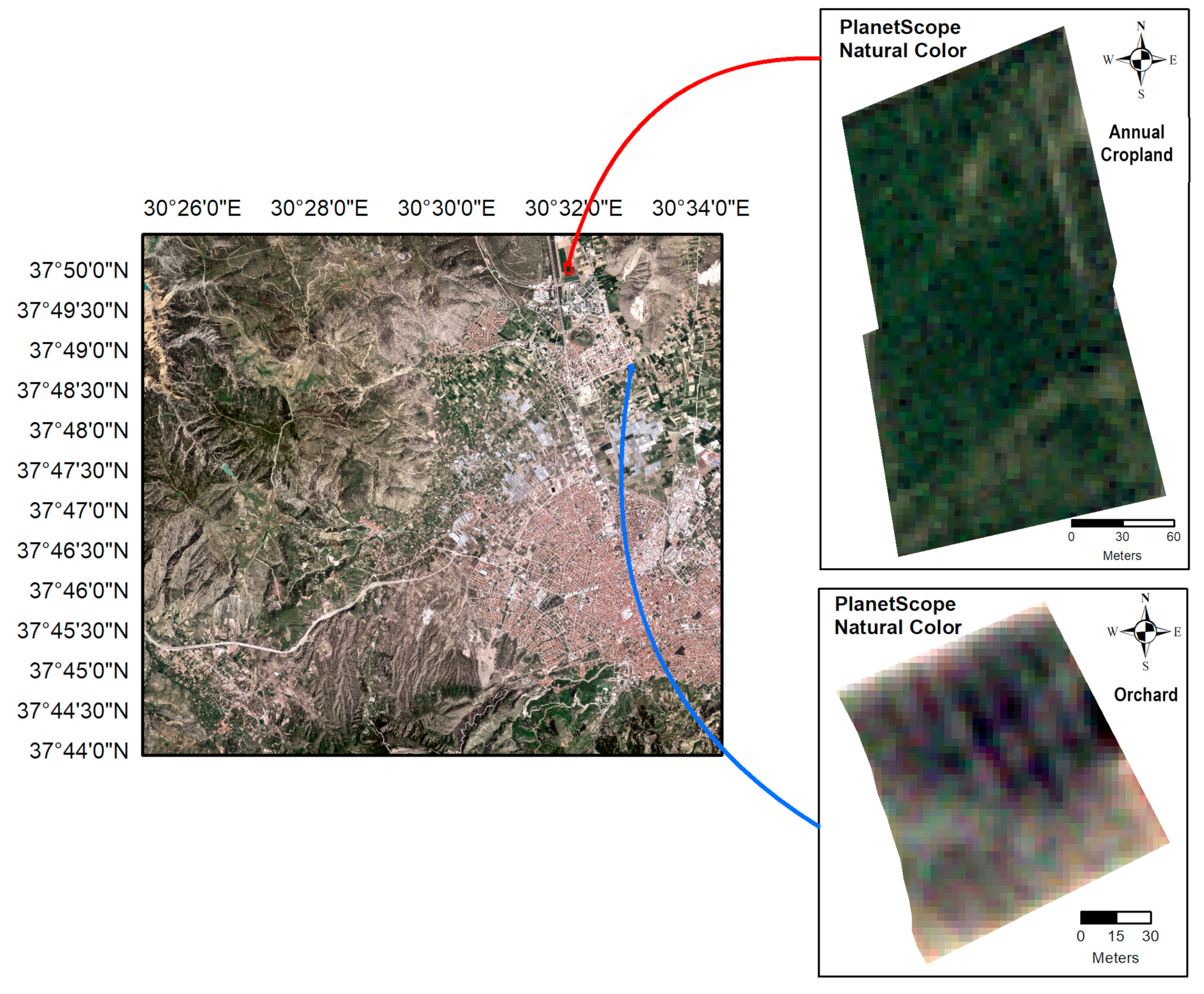
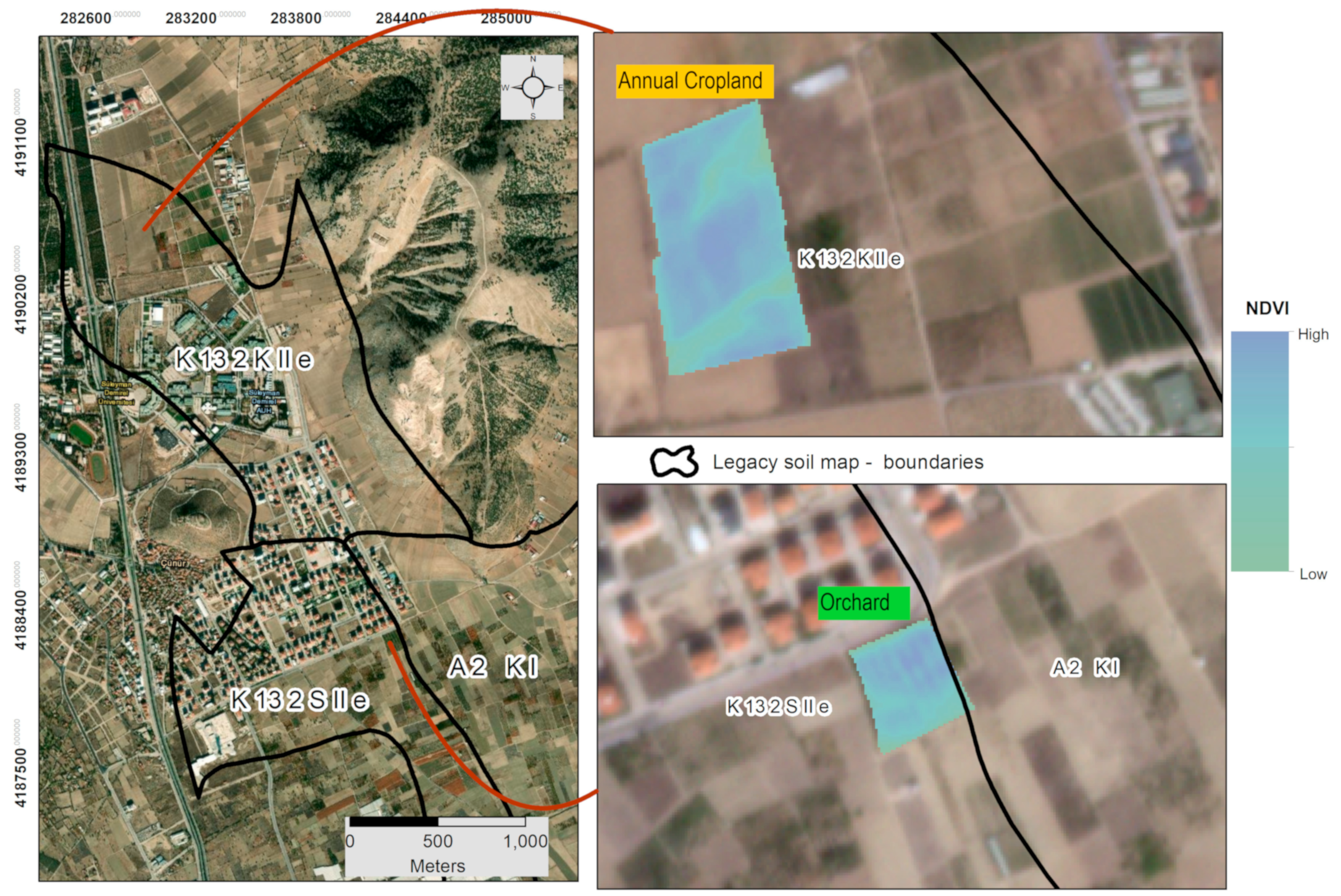
2.1. Study Area

An area of ~4 ha cropland and an area of ~2 ha orchard, representative of smallholder farming in Türkiye, were chosen as the study area (Figure 1). The study area falls under the hot-summer Mediterranean (Csa) climate type, as defined by the Köppen–Geiger climate classification system [26]. The crop rotation for the past three growing seasons in the cropland was durum wheat (Triticum durum), oats (Avena sativa), and barley (Hordeum vulgare). The orchard was used to grow apples (Malus domestica).

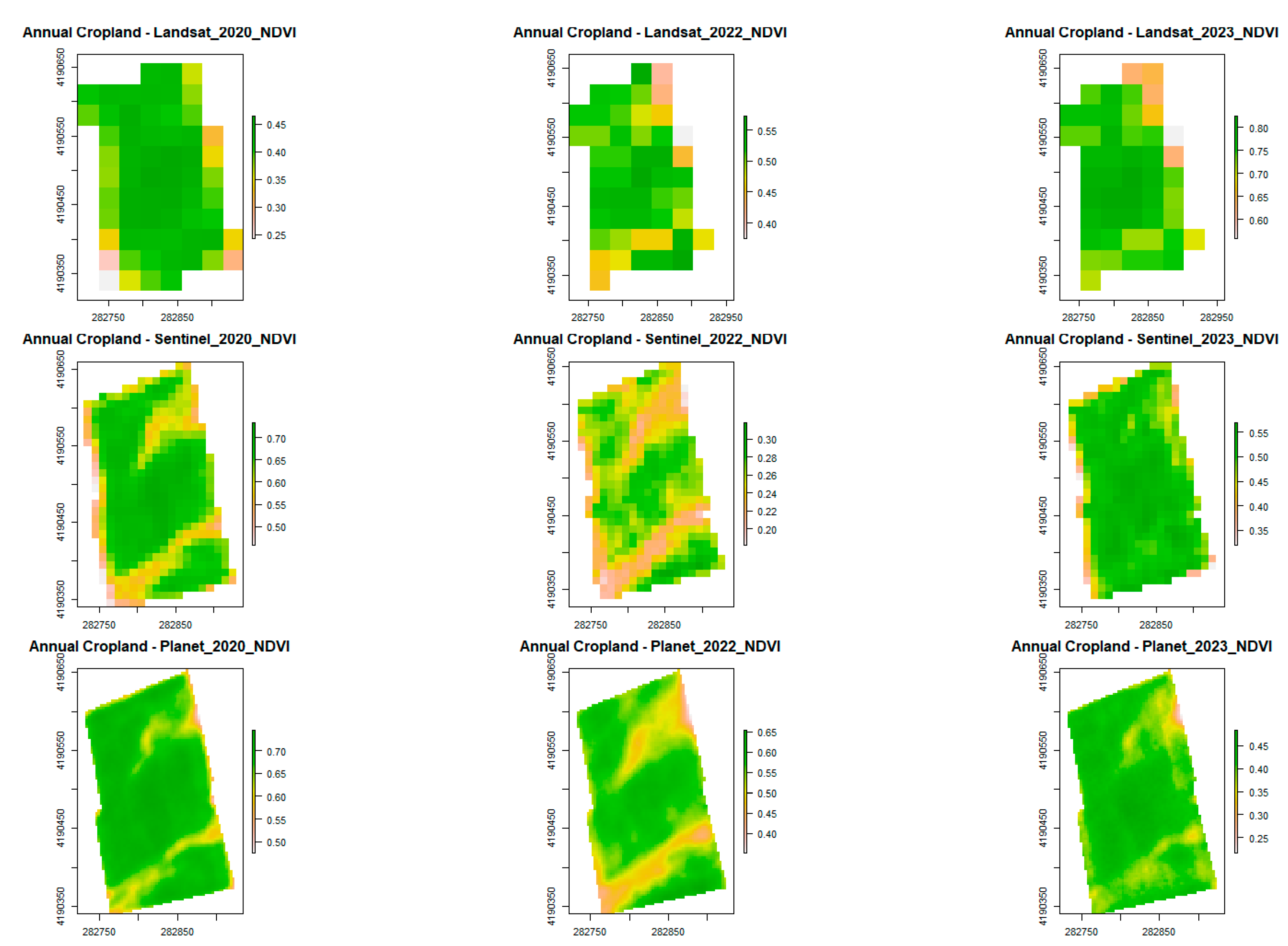
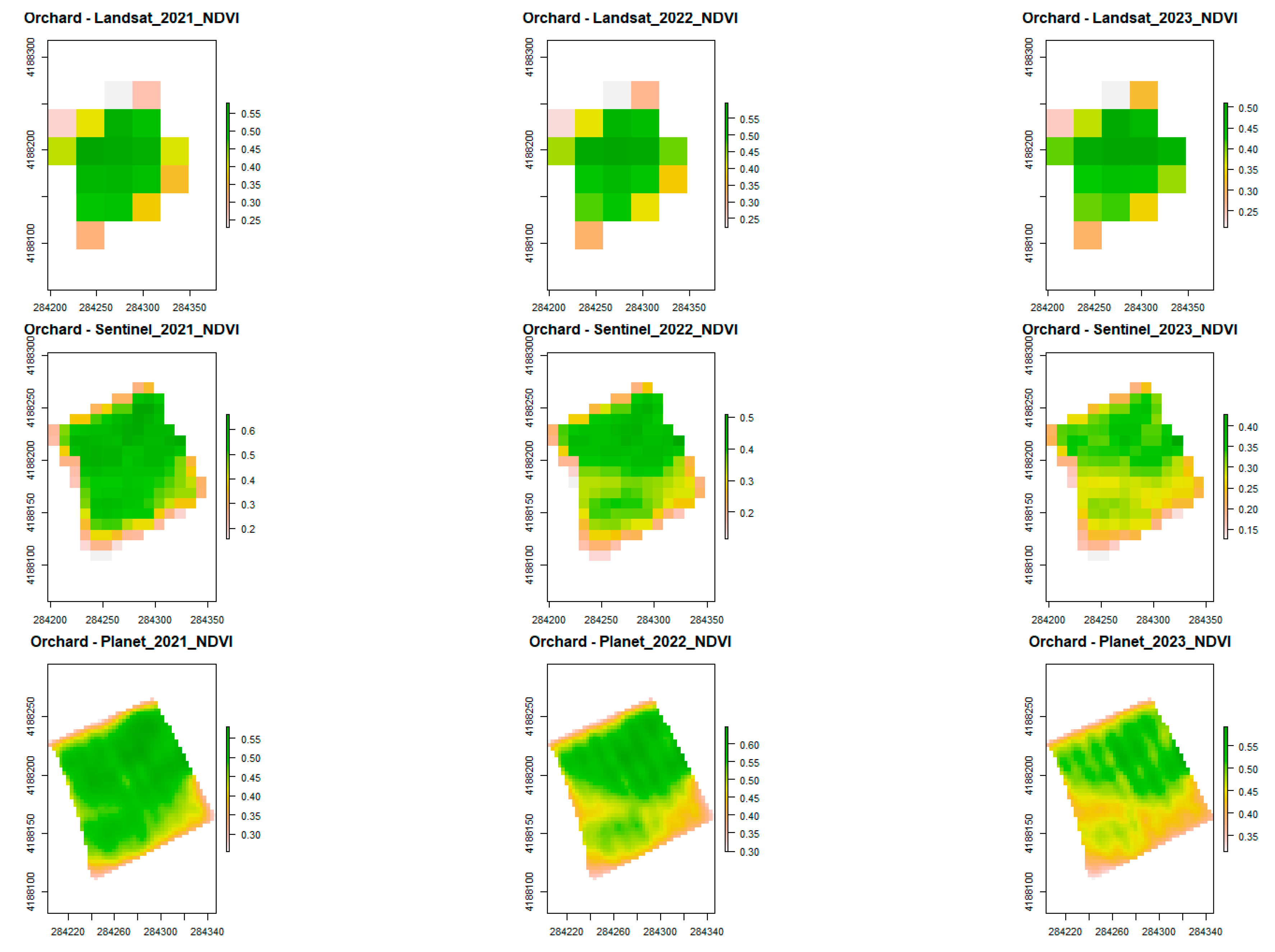
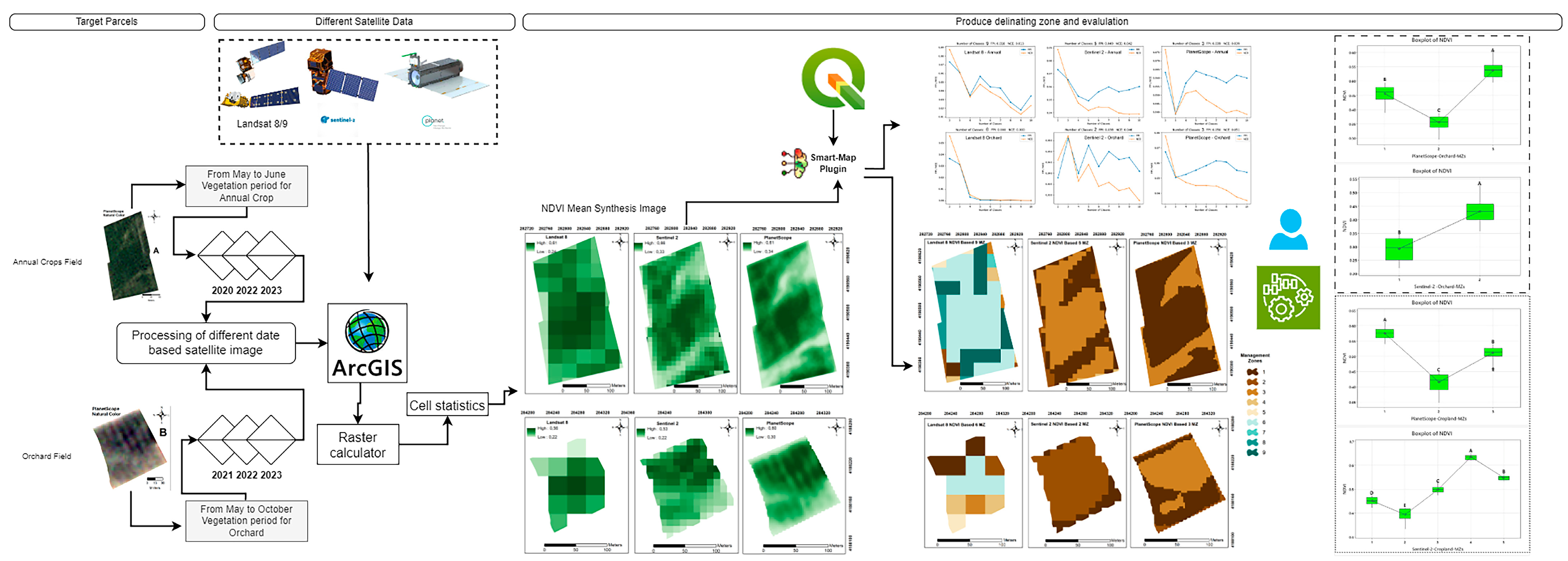
2.2. Remote Sensing Data

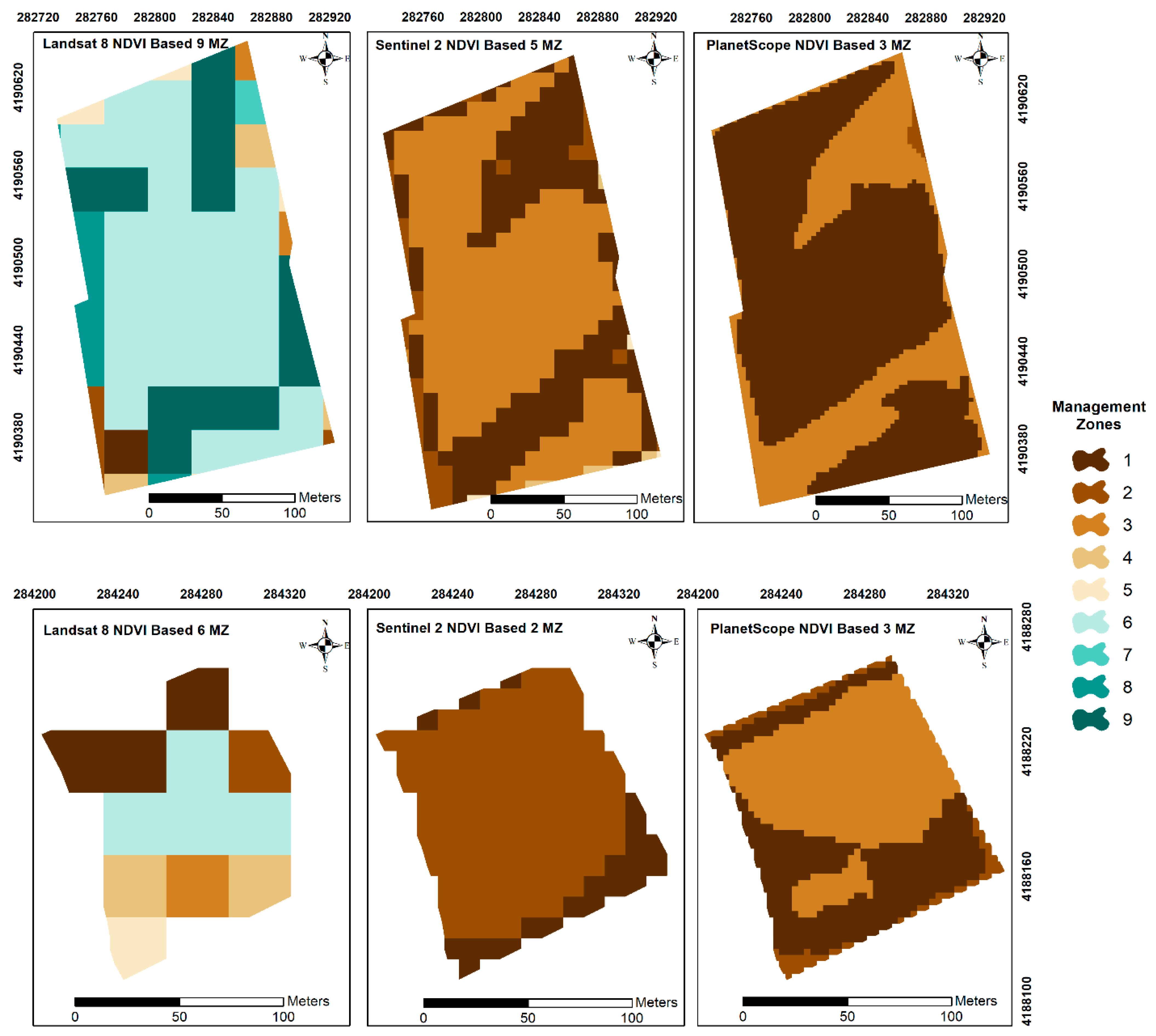
Cloud-free Landsat 8 and Sentinel-2 satellite images were obtained from the Google Earth Engine (GEE) [27], while PlanetScope satellite images were downloaded from Planet Explorer (PE) [28]. The specifications of the satellite images used in this study can be found in

Table 1. Sensor types and metafile information of used satellite images.

Satellite	Annual Cropland	Orchard	Relevant Band Properties
	Month—Year—Image Number	Month—Year—Image Number
Landsat 8	April—2020—1 May—2020—1 June—2020—0	May—2021—1/June—2021—1 July—2021—1/August—2021—1 September—2021—2/October—2021—1	Spatial resolution: 30 m Temporal resolution: 16 days Red Band Spectral resolution: 0.636–0.673 μm NIR Band Spectral resolution: 0.851–0.879 μm Radiometric resolution: 12 bits [30]
	April—2022—0 May—2022—1 June—2022—1	May—2022—0/June—2022—1 July—2022—2/August—2022—1 September—2022—2/October—2022—1
	April—2023—0 May—2023—1 June—2023—0	May—2023—0/June—2023—1 July—2023—2/August—2023—2 September—2023—1/October—2023—0
Sentinel-2	April—2020—2 May—2020—2 June—2020—1	May—2021—6/June—2021—7 July—2021—10/August—2021—11 September—2021—9/October—2021—5	Spatial resolution: 10 m Temporal resolution: 5 days Red Band Spectral resolution: 0.665 μm (Central wavelength) NIR Band Spectral resolution: 0.842 μm (Central wavelength) Radiometric resolution: 12 bits [34]
	April—2022—7 May—2022—7 June—2022—2	May—2022—7/June—2022—4 July—2022—11/August—2022—11 September—2022—10/October—2022—4
	April—2023—3 May—2023—3 June—2023—0	May—2023—1/June—2023—5 July—2023—11/August—2023—12 September—2023—8/October—2023—5
PlanetScope	April—2020—5 May—2020—5 June—2020—1	May—2021—4/June—2021—3 July—2021—3/August—2021—6 September—2021—4/October—2021—4	Dove-R—PS2.SD and SuperDove—PSB.SD Spatial resolution: 3.7 m Temporal resolution: 1 day Red Band Spectral resolution: 0.650–0.682 μm NIR Band Spectral resolution: 0.845–0.888 μm Radiometric resolution: 12 bits [29]
	April—2022—0 May—2022—7 June—2022—3	May—2022—3/June—2022—3 July—2022—3/August—2022—3 September—2022–3/October—2022—3
	April—2023—2 May—2023—4 June—2023—3	May—2023—2/June—2023—8 July—2023—9/August—2023—9 September—2023—9/October—2023—0

. No additional atmospheric and radiometric processes were applied because the images had already been corrected for image artifacts. The satellite images were downloaded during the growing season of the crops in the cropland and orchards. The active ripening season for apples in the orchard was between May and October in 2021, 2022, and 2023, while the growing season in the cropland was between April and mid-June in 2020, 2022, and 2023 (Figure A1 and Figure A2 in Appendix A). The images were downloaded during these periods in the specified years per field. The cropland field was not cultivated in 2021. These months are the most active periods of vegetative growth for croplands and orchards in western Türkiye. The combined effect of cloud cover and temporal resolutions of satellites (i.e., Landsat 8: ~16 days/image, Sentinel-2: ~5 days/image, Planet: 1 day/image) determined the number of available images [29,30,31]. The basic metadata of satellite images is presented in Table 1. All available images obtained per satellite sensor were grouped, and the mean normalized difference vegetation index (NDVI, calculated per group of images using Equation (1) [32]) was determined using the raster calculator in the ArcGIS 10.8.2 software [33].

$$\mathrm{NDVI}={\displaystyle \frac{(\mathrm{N}\mathrm{I}\mathrm{R}-\mathrm{R})}{(\mathrm{N}\mathrm{I}\mathrm{R}+\mathrm{R})}}$$

(1)

In the NDVI calculation, the growing season means near-infrared (NIR) and red (R) bands per group of images from each satellite. For the Landsat 8 satellite, near-infrared (NIR) corresponds to “Band 5”, and red (R) corresponds to “Band 4” [30]. For the Sentinel-2 satellite, near-infrared (NIR) corresponds to “Band 8”, and red (R) corresponds to “Band 4” [34]. There are four bands and eight band images available for the PlanetScope satellite. Accordingly, for the four-band PlanetScope satellite, near-infrared (NIR) corresponds to “Band 4”, and red (R) corresponds to “Band 3”. For the eight-band PlanetScope satellite, near-infrared (NIR) corresponds to “Band 8”, and red (R) corresponds to “Band 6” [29].

2.3. Generating MZs

To delineate the MZs based on the imagery-derived NDVIs with different spatial resolutions (Landsat 8 with 30 m, Sentinel-2 with 10 m, and PlanetScope with 3.7 m), a fuzzy c-means clustering algorithm was used the Smart-Map tool developed by Pereira et al. [35] in the QGIS software (version 3.2) [36]. The Smart-Map plugin calculates the fuzziness performance index (FPI) and normalized classification entropy (NCE), which are widely accepted in the literature to determine the optimal number of MZs [35]. The FPI gauges the extent of overlap among various categories (fuzziness: [37]). NCE has been developed as a metric to measure the degree of uncertainty or randomness in cluster assignments. It has been demonstrated that lower values of NCE are indicative of more reliable and well-defined clusters. The NCE is employed to determine the optimal number of clusters for creating MZs, aiding users in generating MZs efficiently [38]. The convergence of FPI and NCE corresponds to the optimal MZ number.

Figure 2 presents the delineation process of MZs based on mean NDVI images generated from time-series satellite images. The process begins with the acquisition of satellite imagery focused on the vegetative stages, with a particular emphasis on the study plots. Vegetative stages may vary depending on the choice of region for the study area in future studies. The calculation of relevant year NDVI averages for the vegetative periods within the selected areas then followed. The utilization of three-year data necessitates an iteration, resulting in the generation of a final three-year NDVI average (synthesis) image. This final synthesis image constitutes the primary input for the Smart-Map Plugin [39], and the fuzzy-c-means analysis is conducted on this data. The process concludes by generating quantitative cluster evaluation criteria and spatial maps of the clusters.

2.4. Statistical Analysis for Comparing MZs

Mean NDVI pixels under two different agricultural management practices (cropland and orchard) were converted to point data using the ArcGIS ArcMap 10.8.2 Raster to Point (Conversion) tool [33]. The MZs that these points fall into were determined with the Extract Multi Values to Points (Spatial Analyst) tool [33]. Based on this dataset, the NDVI mean values were calculated for each MZ produced based on different satellite images under two different agricultural management systems (cropland and orchard). A variance analysis was performed separately for each satellite and each agricultural management. Assumptions were checked before the variance analysis. After confirming the normal distribution of the data, Bartlett’s method was used for the assumption of equality/homogeneity of the variances. The assumption of equality/homogeneity of the variances was valid only for Sentinel-2 orchard MZs. A one-way ANOVA was conducted for the Sentinel-2 orchard MZs. For the others, equal variances could not be assumed in the analysis, and Welch’s ANOVA was conducted. Tukey’s (p < 0.05) method was used in a one-way ANOVA, and Games-Howell’s (p < 0.05) method was used in Welch’s ANOVA for grouping. Statistical analyses were conducted in the Minitab Statistical Software (21.2.0.0). Considering

Table 2. Evaluation of clustering results, including fuzzy c-means, in terms of FPI, NCI, and Pixels per Cluster.

Sensor	Cultivation Type	Cluster Number	FPI	NCE	Pixel Count	Pixels per Cluster (Approximate)
Landsat 8	Annual Cropland	9	0.018	0.013	63	7
	Orchard	6	0.000	0.000	12	2
Sentinel-2	Annual Cropland	5	0.049	0.042	456	91
	Orchard	2	0.038	0.046	126	63
PlanetScope	Annual Cropland	3	0.039	0.039	4650	1550
	Orchard	3	0.050	0.051	1404	468

FPI: fuzziness performance index; NCE: normalized classification entropy.

, since the number of NDVI observations in Landsat 8-based MZs was quite low, the mean comparison process was not conducted.

3. Results

The minimum NDVI values for annual cropland ranged from 0.24 to 0.34 among the three satellite sensors, while the maximum NDVI values ranged from 0.61 to 0.66 across the two study areas (Figure 3). Similarly, the minimum NDVI values for orchards ranged from 0.22 to 0.30, while the maximum NDVI values were in the range of 0.53 to 0.60. The minimum NDVI values for orchards were lower than those for cropland among the three sensors. In the cropland parcel, from late May to mid-June, the soil’s reflection will be considerably low because this is the period when barley ripens and covers the soil surface. However, in an orchard parcel with apple trees from May to October, the presence of bare soil between and within rows will influence the reflection of NIR and red bands [40]. PlanetScope and Sentinel-2 generate relatively similar NDVI patterns for both annual cropland and orchard parcels, but the NDVI from PlanetScope contains finer details.

Quantitative evaluation metrics of the fuzzy c-means cluster analysis are presented in Figure 4. All the sensors determined a different number of MZs, as each determined a unique count, as indicated by the lowest values of the NCE and FPI metrics (Figure 4). Landsat 8 was found to generate a higher number of clusters compared to the other two sensors, both in the context of annual cropland and orchard plots (Figure 4 and Table 2). Given that the research was conducted at the plot level, Landsat 8 could represent annual cropland with approximately 60 pixels, while orchards could be represented with only 12 pixels (Table 2).

While this result may be specific to the current study, it is noteworthy that higher cluster numbers were obtained using a reduced number of observations (Table 2). Consequently, the practical implementation of high cluster numbers in the context of parcel-scale management is not feasible, as it would necessitate the establishment of numerous MZs. In the current study, the delineation of nine MZs within a 4 ha annual cropland area and six MZs within a 2 ha orchard area are not practical (Table 2 and Figure 5). The attribution of meaning to each cluster is possible through the acquisition by soil scientists of soil data specific to the cluster. The clusters produced by this methodology can be defined as potential MZs and provide insight for farmers at the parcel scale.

The patterns in MZs were affected by the spatial resolution (Figure 5). Visually, the PlanetScope-based map provided finer details, while Landsat 8 led to coarser spatial patterns in the resultant MZ maps within cropland parcels (Figure 5). The number of clusters that could be depicted as MZs tended to decrease with a higher spatial resolution (Figure 5) and a higher pixel count (Table 2) in both parcels.

As the MZs in Figure 5 are yet to be interpreted in the context of soil information, the clusters in each plot have not been schematized in different colors. An evaluation of the number and pattern of MZs in this study can be considered sufficient. The similarity in the pattern of MZs based on PlanetScope and Sentinel-2 satellite images in Figure 5 for both orchard and annual cropland is remarkable. Notably, the optimal natural boundaries identified for the formation of an MZ according to NDVI were obtained by using PlanetScope.

NDVI showing different MZs is highly important but is useless without knowing the potential causes. The potential cause may be, as emphasized here, a difference in the edaphic soil properties. Our findings indicate that one of the parcel-specific MZs in both areas consists of pixels at the edges of the parcel (Figure 5). Compared to other sensors, the fact that Landsat 8 pixels contained more area from the field edges due to the coarse spatial resolution may be misleading when reflecting in-field NDVI variations. The effect of parcel boundaries should not be ignored here. Parcel boundaries are significantly affected by the reflections of neighboring parcels when spatial resolution is considered. The variation in MZs could be attributed to the variation in soil. However, it is necessary to consider the sensitivity of the clustering algorithm to the distribution of the NDVI mean values (Figure 6).

Table 3. Results of analysis conducted with equal variances assumed in one-way ANOVA and equal variances not assumed in Welch’s ANOVA.

Sentinel-2 Orchard MZs—one-way ANOVA
Grouping *	MZs	N	Mean	StDev	95% CI	DF	R-sq(adj)	F-Value	p-Value
B	1	22	0.29	0.04	(0.276; 0.308)	1	64.73%	230.46	0.000
A	2	104	0.43	0.03	(0.422; 0.437)
PlanetScope Orchard MZs—Welch’s ANOVA
Grouping	MZs	N	Mean	StDev	95% CI	DF	R-sq(adj)	F	p
B	1	566	0.46	0.03	(0.453; 0.458)	2	80.62%	3328.29	0.000
C	2	94	0.36	0.02	(0.351; 0.360)
A	3	744	0.54	0.03	(0.535; 0.538)
Sentinel-2 Cropland MZs—Welch’s ANOVA
Grouping	MZs	N	Mean	StDev	95% CI	DF	R-sq(adj)	F	p
D	1	155	0.45	0.01	(0.448; 0.453)	4	88.02%	667.50	0.000
E	2	37	0.39	0.02	(0.385; 0.401)
C	3	249	0.50	0.01	(0.496; 0.499)
A	4	8	0.63	0.01	(0.623; 0.645)
B	5	7	0.55	0.01	(0.537; 0.558)
PlanetScope Cropland MZs—Welch’s ANOVA
Grouping	MZs	N	Mean	StDev	95% CI	DF	R-sq(adj)	F	p
A	1	3209	0.57	0.01	(0.574; 0.575)	2	74.82%	5996.17	0.000
C	2	35	0.42	0.03	(0.406; 0.425)
B	3	1406	0.51	0.02	(0.510; 0.512)

* Different letters are significantly different at the p ≤ 0.05 level of significance as per Tukey’s method in the one-way ANOVA, while different letters are significantly different at the p ≤ 0.05 level of significance as per Games-Howell’s method in Welch’s ANOVA. Abbreviations. MZs: management zones; N: number of observations; StDev: standard deviation; CI: confidence interval; DF: degrees of freedom; R-sq(adj): adjusted R-squared.

shows the results of a comparative ANOVA conducted on the means of fuzzy-c-means-based MZs generated using NDVI data from satellite images at different spatial resolutions in orchard and cropland areas. The one-way ANOVA and Welch’s ANOVA results show that there are statistically significant differences (p < 0.05) between the NDVIs derived from MZs using Sentinel-2 and PlanetScope. Sentinel-2 produced more MZs for cropland (five MZs) (Table 3). There are statistically significant differences between the groups (p < 0.05) (Table 3). The region with the highest NDVI mean is MZ 4, while the lowest is MZ 2 (Table 3). The Welch ANOVA test for Sentinel-2 cropland MZs revealed that statistically significant differences were found among MZ 1 (0.45), MZ 2 (0.39), MZ 3 (0.50), MZ 4 (0.63), and MZ 5 (0.55) (F = 667.50, p = 0.000) (Table 3). The Welch ANOVA test for PlanetScope cropland MZs showed that there were statistically significant differences between MZ 1 (0.57), MZ 2 (0.42), and MZ 3 (0.51) (F = 5996.17, p = 0.000) (Table 3). In the cropland area, MZ 4 and MZ 2 are spatially separable (Figure 5). A similar separation is also present in the PlanetScope satellite (Figure 5). In the cropland, Sentinel-2 explained about 88% of the variation with five MZs, while PlanetScope explained about 75% with three MZs (Table 3). Sentinel-2 was able to identify only two MZs in the orchard, and these MZs had statistically significant differences in NDVI (p < 0.05). The one-way ANOVA test for the Sentinel-2 orchard MZs found a statistically significant difference between MZ 1 (0.29) and MZ 2 (0.43) (F = 230.46, p = 0.000) (Table 3). The higher-resolution PlanetScope made a more detailed distinction in the orchard areas than Sentinel-2, creating three MZs (Table 3) in the orchards. While PlanetScope explained approximately 81% of the variation using three MZs in the orchard areas, Sentinel-2 explained approximately 65% of the variation with two MZs (Table 3). In the orchards, it is seen that PlanetScope detects more details compared to Sentinel-2 because of its higher resolution. Welch’s ANOVA test for PlanetScope orchard MZs showed statistically significant differences between MZ 1 (0.46), MZ 2 (0.36), and MZ 3 (0.54) (F = 3328.29, p = 0.000) (Table 3). As a result of these findings, the null hypothesis (H₀) was rejected, and the alternative hypothesis (H₁) was accepted. These findings support the idea that higher-resolution satellite data can offer clearer distinctions between MZs and that MZs are statistically significant different in terms of NDVI values.

4. Discussion

As a result of the cluster analysis conducted using the average NDVI based on satellite images, the clusters produced were evaluated with ANOVA. The wider spectral coverage of Sentinel-2, which has around 10 m of spatial resolution, may enable it to detect more heterogeneity in large-scale agricultural areas. The spatial resolution of PlanetScope, around 3 m, may have captured more detailed variability, especially in the orchards. The MZ map using only RS data can provide preliminary information to distinguish soil qualities, i.e., there is a potential to differentiate between heterogeneous soil regions. This approach reveals that the spatial resolution of remote sensing products is effective in different management practices to delineate MZs in precision agriculture. While Sentinel-2 provides better separation MZs for croplands, PlanetScope can create more MZs in gardens. Differences in NDVI are statistically (p < 0.05) significant differences present among MZs. Delineation of MZs is a critical step for precision agriculture practices, and different satellite images provide information at different scales.

The farming history (e.g., fertilizer applications, annual rotation, age of the trees, etc.) and spatial variation of soil properties in the study area have significant effects on crop yield, and these factors are potentially related to NDVI maps. Previous studies have shown that NDVI maps are suitable predictors of MZs that can account for these variations and ultimately predict crop yield [16]. Despite that, the spatial resolution of input imagery for creating NDVI maps will ultimately determine the level of detail in the resulting MZs. In PA, the scale of observation that best suits the farmer’s requirements should be chosen. For example, maps generated from medium spatial resolution data can support rapid decisions at relatively larger scales, for example, at the town scale [5]. On the other hand, parcel-level agricultural management would demand finer resolution imagery to create MZs. Other studies also recognized this need [6,7,20]. Studies such as Mohr et al. [18] with RapidEye imagery and others using PlanetScope-based NDVI [6,23] have confirmed that high-resolution imagery effectively captures in-field variability. Consistent with previous studies, our study highlights that higher spatial resolution enhances crop monitoring and vigor assessments [23].

Remote sensing tracks plant growth and soil responses for precision agriculture. In developing countries, like Türkiye, the transition to digital agriculture from conventional farming is gaining momentum among farmers who effectively utilize mobile devices. As a result, some Turkish start-ups [11,12,13] use Sentinel-2 data to provide farmers with NDVI data for their parcels, allowing them to monitor crop health effectively. To support this transition, we evaluated different sensors from coarse to finer resolution imagery to develop a low-cost method to delineate MZs in cropland and orchard parcels based on the unsupervised image classification of the multi-temporal vegetation index. The impact of spatial resolution on the determination of MZs was assessed in a smallholder farm in southwestern Türkiye. Our findings show that resolution has a substantial impact on the stability of resulting MZs. Finer resolution imagery (PlanetScope) not only provides greater details in NDVI maps but, more importantly, better stability in the resulting MZs. This proved the usefulness of PlanetScope imagery compared to other sensors in creating MZs at the parcel scale. Although finer resolution imagery has led to a more detailed identification of MZs, Sentinel-2 imagery, which is relatively coarser than PlanetScope imagery, can be used where the area is large and there are financial constraints.

In some studies, other vegetation indices exhibited superiority to NDVI in MZ delineation, a noteworthy finding [40]. Segarra et al. [41] conducted a study focusing on parcel-based yield zones of winter cereals in the northern inner plateaus of Spain. They reported that the biophysical parameter Leaf Area Index (LAI), obtained from radiative transfer models (RTMs) based on Sentinel-2 bands, showed slightly better performance in representing within-field heterogeneity compared to NDVI. Singh et al. [42] developed digital suitability zones using Sentinel-2 data for planning expansion areas in small-scale cocoa agriculture. There are aspects worth further investigation concerning the effectiveness of vegetation indices that incorporate red-edge bands [43], which contain more unique information about plant vitality, in creating MZs for both cropland and orchard agricultural cultivation types.

Future studies on MZs delineation can focus on validating the resulting MZs with soil sampling or yield data. For example, MZs were based on PlanetScope imagery and ISODATA, and the resultant MZs were validated with soil sampling data using statistical mean difference via the Tukey honestly significant difference (HSD) test [1,44]. This was because attributes derived from soil sampling are considered essential for improving the quality of MZ identification by supplementing the use of sensor-based inputs (e.g., NDVI maps) [45]. Another area of improvement in MZ maps could be to smooth the resulting maps by integrating smaller fractions of specific zones into more dominant zones. This could, in turn, ease and improve agricultural decision-making. For both croplands and orchards, remote sensing-based MZs can serve as a practical guide to understanding existing within-field soil variability and managing that variability [46].

This study aimed to assess the performance of different satellite images in MZ delineation while noting the need for validating resulting MZs with ground-truth data, such as soil samples. Notably, variations in MZs within the study area may be attributed to soil physical properties. Specifically, in zones 2 and 3 (Figure 5), the variations in MZs could be attributed to soil physical properties. In attempts to integrate earth observation data and use soil science knowledge for decision-making in soil fertility management, it is important to make comparative analysis with legacy data specific to the study areas. The study areas are characterized by colluvial and alluvial soils (Figure 7). These areas are classified as deep- and medium-textured soils [(K 13: colluvial, loamy texture) and (A 2: alluvial, loamy texture)] in the Land Inventory Report [47]. Although it is challenging to integrate legacy maps into the decision support system at the parcel scale due to their coarse resolution (Figure 7), high-spatial-resolution imagery can provide much greater details for PA applications. Given the alluvial physiography of the study area, minor changes in slope significantly influence surface flow patterns. Furthermore, in the orchard (apple) areas, characterized by alluvial physiography, noticeable changes in soil texture are observed over short distances. The effects of these changes in edaphic factors on crop growth can be determined spatially by using high-resolution satellite images.

Small farm parcels often exhibit high soil heterogeneity that remains poorly identified. Hence, there is a need for local characterization based on both local and scientific knowledge [48]. In both croplands and orchards, remote sensing-based MZs can serve as a practical guide to deciding how to manage soil variability, primarily by acknowledging that plant reflectance indicates variation in the soil [49]. The MZs in our study are the outcome of multiyear satellite imagery-based mean NDVI maps. The abundance of available historical earth observation data enables the creation of long-term NDVI averages [50]. However, this process requires substantial computational capacity. The presence of efficient cloud-based platforms for geographic data analysis and processing, such as Google Earth Engine [27] and Microsoft Planetary Computer [51], could facilitate and optimize this process. Given the accessibility of openly available satellite data and their effective processing capacities, these two cloud-based tools should be investigated for their efficacy in future research endeavors [52].

This study highlights the impact of spatial resolution on MZ delineation while demonstrating how the sensitivity of the fuzzy c-means clustering algorithm used to analyze the data distribution can affect the results (Table 2). Specifically, while the pixel numbers for the parcels having Landsat 8 ranged from 12 to 63, the PlanetScope data revealed a broader range of pixel numbers from 1404 to 4650 (Table 2). A key limitation of the present study is the need for a comparative evaluation of the performance of various clustering algorithms [53]. Additionally, given our emphasis on the parcel scale, further studies can integrate a wider variety of parcel sizes and optimize parcel sizes.

5. Conclusions

This study compared the ability of sensors with coarse, medium, and fine spatial resolutions to detect within-parcel heterogeneity of edaphic factors using NDVI maps as proxies. To enable low-input and efficient MZ mapping for cropland and orchard parcels, an open-source workflow was applied to process NDVI maps and delineate MZs. PlanetScope satellites, with their relatively higher spatial resolution, consistently produced comparable and reliable MZs across orchard areas. In contrast, Landsat 8 imagery, due to its coarse spatial resolution and edge effects, generated excessive and less meaningful MZs. The findings highlight the importance of exploring how satellite imagery can be used to monitor and control plant growth within MZs. Future studies should focus on understanding plant responses to soil properties through remote sensing strategies to optimize soil management.

References

1. Ferhatoglu, C. Delineating Precision Agriculture Management Zones Using Satellite Imagery, Web Soil Survey, and Machine Learning. Master’s Thesis, North Carolina State University, Raleigh, NC, USA, 2019. [Google Scholar]
2. Corti, M.; Gallina, P.M.; Cavalli, D.; Ortuani, B.; Cabassi, G.; Cola, G.; Vigoni, A.; Degano, L.; Bregaglio, S. Evaluation of In-Season Management Zones from High-Resolution Soil and Plant Sensors. Agronomy 2020, 10, 1124. [Google Scholar] [CrossRef]
3. Georgi, C.; Spengler, D.; Itzerott, S.; Kleinschmit, B. Automatic Delineation Algorithm for Site-Specific Management Zones Based on Satellite Remote Sensing Data. Precis. Agric. 2018, 19, 684–707. [Google Scholar] [CrossRef]
4. Guo, Y.; Shi, Z.; Li, H.Y.; Triantafilis, J. Application of Digital Soil Mapping Methods for Identifying Salinity Management Classes Based on a Study on Coastal Central China. Soil Use Manag. 2013, 29, 445–456. [Google Scholar] [CrossRef]
5. Cammarano, D.; Zha, H.; Wilson, L.; Li, Y.; Batchelor, W.D.; Miao, Y. A Remote Sensing-Based Approach to Management Zone Delineation in Small Scale Farming Systems. Agronomy 2020, 10, 1767. [Google Scholar] [CrossRef]
6. Breunig, F.M.; Galvão, L.S.; Dalagnol, R.; Dauve, C.E.; Parraga, A.; Santi, A.L.; Della Flora, D.P.; Chen, S. Delineation of Management Zones in Agricultural Fields Using Cover–Crop Biomass Estimates from PlanetScope Data. Int. J. Appl. Earth Obs. Geoinf. 2020, 85, 102004. [Google Scholar] [CrossRef]
7. Catania, P.; Ferro, M.V.; Orlando, S.; Vallone, M. Grapevine and Cover Crop Spectral Response to Evaluate Vineyard Spatio-Temporal Variability. Sci. Hortic. 2025, 339, 113844. [Google Scholar] [CrossRef]
8. Fridgen, J.J.; Kitchen, N.R.; Sudduth, K.A.; Drummond, S.T.; Wiebold, W.J.; Fraisse, C.W. Management Zone Analyst (MZA). Agron. J. 2004, 96, 100–108. [Google Scholar] [CrossRef]
9. Sozzi, M.; Kayad, A.; Giora, D.; Sartori, L.; Marinello, F. Cost-Effectiveness and Performance of Optical Satellites Constellation for Precision Agriculture. In Precision Agriculture 2019—Papers Presented at the 12th European Conference on Precision Agriculture, ECPA 2019; Wageningen Academic: Leiden, The Netherlands, 2019; pp. 501–507. [Google Scholar] [CrossRef]
10. OneSoil. Available online: https://onesoil.ai/en (accessed on 10 November 2024).
11. Doktar. Available online: https://www.doktar.com/tr/orbit-uydudan-takip (accessed on 10 November 2024).
12. KORBİS. Available online: https://tarimkredi.org.tr/faaliyetler/korbis/ (accessed on 10 November 2024).
13. Tarla.Io. Available online: https://www.tarla.io/tr-TR (accessed on 10 November 2024).
14. Mendes, J.; Pinho, T.M.; Dos Santos, F.N.; Sousa, J.J.; Peres, E.; Boaventura-Cunha, J.; Cunha, M.; Morais, R. Smartphone Applications Targeting Precision Agriculture Practices—A Systematic Review. Agronomy 2020, 10, 855. [Google Scholar] [CrossRef]
15. Filippi, P.; Whelan, B.M.; Bishop, T.F.A. Proximal and Remote Sensing—What Makes the Best Farm Digital Soil Maps? Soil Res. 2024, 62, SR23112. [Google Scholar] [CrossRef]
16. Damian, J.M.; Pias, O.H.d.C.; Cherubin, M.R.; Fonseca, A.Z.d.; Fornari, E.Z.; Santi, A.L. Applying the NDVI from Satellite Images in Delimiting Management Zones for Annual Crops. Sci. Agric. 2020, 77, e20180055. [Google Scholar] [CrossRef]
17. Termin, D.; Linker, R.; Baram, S.; Raveh, E.; Ohana-Levi, N.; Paz-Kagan, T. Dynamic Delineation of Management Zones for Site-Specific Nitrogen Fertilization in a Citrus Orchard. Precis. Agric. 2023, 24, 1570–1592. [Google Scholar] [CrossRef]
18. Mohr, J.; Tewes, A.; Ahrends, H.; Gaiser, T. Assessing the Within-Field Heterogeneity Using Rapid-Eye NDVI Time Series Data. Agriculture 2023, 13, 1029. [Google Scholar] [CrossRef]
19. Song, X.; Wang, J.; Huang, W.; Liu, L.; Yan, G.; Pu, R. The Delineation of Agricultural Management Zones with High Resolution Remotely Sensed Data. Precis. Agric. 2009, 10, 471–487. [Google Scholar] [CrossRef]
20. Fletcher, R.S.; Escobar, D.E.; Skaria, M. Evaluating Airborne Normalized Difference Vegetation Index Imagery for Citrus Orchard Surveys. Horttechnology 2004, 14, 91–94. [Google Scholar] [CrossRef]
21. Reyes, F.; Casa, R.; Tolomio, M.; Dalponte, M.; Mzid, N. Soil Properties Zoning of Agricultural Fields Based on a Climate-Driven Spatial Clustering of Remote Sensing Time Series Data. Eur. J. Agron. 2023, 150, 126930. [Google Scholar] [CrossRef]
22. Rodrigues, H.; Ceddia, M.B.; Vasques, G.M.; Mulder, V.L.; Heuvelink, G.B.M.; Oliveira, R.P.; Brandão, Z.N.; Morais, J.P.S.; Neves, M.L.; Tavares, S.R.L. Remote Sensing and Kriging with External Drift to Improve Sparse Proximal Soil Sensing Data and Define Management Zones in Precision Agriculture. AgriEngineering 2023, 5, 2326–2348. [Google Scholar] [CrossRef]
23. Breunig, F.M.; Galvão, L.S.; Dalagnol, R.; Santi, A.L.; Della Flora, D.P.; Chen, S. Assessing the Effect of Spatial Resolution on the Delineation of Management Zones for Smallholder Farming in Southern Brazil. Remote Sens. Appl. 2020, 19, 100325. [Google Scholar] [CrossRef]
24. Chatzidavid, D.; Kokinou, E.; Gerarchakis, N.; Kontogiorgakis, I.; Bucaioni, A.; Bogdanovic, M. Delineation Protocol of Agricultural Management Zones (Olive Trees and Alfalfa) at Field Scale (Crete, Greece). Remote Sens. 2024, 16, 4486. [Google Scholar] [CrossRef]
25. Sapkota, A.; Verdi, A.; Scudiero, E.; Montazar, A. Assessing the Effectiveness of Satellite and UAV-Based Remote Sensing for Delineating Alfalfa Management Zones under Heterogeneous Rootzone Soil Salinity. Smart Agric. Technol. 2024, 9, 100583. [Google Scholar] [CrossRef]
26. Kaya, F.; Schillaci, C.; Keshavarzi, A.; Basayigit, L. Predictive Mapping of Electrical Conductivity and Assessment of Soil Salinity in a Western Türkiye Alluvial Plain. Land 2022, 11, 2148. [Google Scholar] [CrossRef]
27. Gorelick, N.; Hancher, M.; Dixon, M.; Ilyushchenko, S.; Thau, D.; Moore, R. Google Earth Engine: Planetary-Scale Geospatial Analysis for Everyone. Remote Sens. Environ. 2017, 202, 18–27. [Google Scholar] [CrossRef]
28. Planet Team Planet Application Program Interface. Available online: https://www.planet.com/explorer/ (accessed on 8 September 2022).
29. Planet. Planet Imagery Product Specifications. Available online: https://assets.planet.com/docs/Planet_Combined_Imagery_Product_Specs_letter_screen.pdf (accessed on 10 November 2024).
30. Landsat 8 Data Users Handbook|U.S. Geological Survey. Available online: https://www.usgs.gov/media/files/landsat-8-data-users-handbook (accessed on 10 November 2024).
31. Sentinel-2 User Handbook. Issue 1 Revision 1. 2013. Available online: https://sentinel.esa.int/documents/247904/685211/Sentinel-2_User_Handbook (accessed on 10 November 2024).
32. Ashley, M.D.; Rea, J. Seasonal Vegetation Differences from ERTS Imagery. Photogramm. Eng. Remote Sens. 1975, 41, 713–719. [Google Scholar]
33. ESRI. ArcGIS Desktop 10.8.2 Documentation. Environmental Systems Research Institute. Available online: https://desktop.arcgis.com (accessed on 10 November 2024).
34. Sentinel-2 User Handbook; 1.2.; European Space Agency (ESA): Paris, France, 2015.
35. Pereira, G.W.; Valente, D.S.M.; de Queiroz, D.M.; Coelho, A.L.d.F.; Costa, M.M.; Grift, T. Smart-Map: An Open-Source QGIS Plugin for Digital Mapping Using Machine Learning Techniques and Ordinary Kriging. Agronomy 2022, 12, 1350. [Google Scholar] [CrossRef]
36. QGIS Development Team. QGIS Geographic Information System. 2023. QGIS GeographicInformation System. Open-Source Geospatial Foundation Project. Available online: http://qgis.osgeo.org (accessed on 10 November 2024).
37. Odeh, I.O.A.; McBratney, A.B.; Chittleborough, D.J. Soil Pattern Recognition with Fuzzy-c-Means: Application to Classification and Soil-Landform Interrelationships. Soil Sci. Soc. Am. J. 1992, 56, 505–516. [Google Scholar] [CrossRef]
38. Bezdek, J.C. Pattern Recognition with Fuzzy Objective Function Algorithms, 1st ed.; Bezdek, J.C., Ed.; Springer: New York, NY, USA, 1981; ISBN 978-1-4757-0452-5. [Google Scholar]
39. Smart Map (Version 1.4.2) [QGIS plugin]. QGIS Python Plugins Repository. Available online: https://plugins.qgis.org/plugins/Smart_Map/ (accessed on 10 November 2024).
40. Sandonís-Pozo, L.; Llorens, J.; Escolà, A.; Arnó, J.; Pascual, M.; Martínez-Casasnovas, J.A. Satellite Multispectral Indices to Estimate Canopy Parameters and Within-Field Management Zones in Super-Intensive Almond Orchards. Precis. Agric. 2022, 23, 2040–2062. [Google Scholar] [CrossRef]
41. Segarra, J.; Araus, J.L.; Kefauver, S.C. Farming and Earth Observation: Sentinel-2 Data to Estimate within-Field Wheat Grain Yield. Int. J. Appl. Earth Obs. Geoinf. 2022, 107, 102697. [Google Scholar] [CrossRef]
42. Singh, K.; Fuentes, I.; Al-Shammari, D.; Fidelis, C.; Butubu, J.; Yinil, D.; Sharififar, A.; Minasny, B.; Guest, D.I.; Field, D.J. E-Agriculture Planning Tool for Supporting Smallholder Cocoa Intensification Using Remotely Sensed Data. Remote Sens. 2023, 15, 3492. [Google Scholar] [CrossRef]
43. Fassa, V.; Pricca, N.; Cabassi, G.; Bechini, L.; Corti, M. Site-Specific Nitrogen Recommendations’ Empirical Algorithm for Maize Crop Based on the Fusion of Soil and Vegetation Maps. Comput. Electron. Agric. 2022, 203, 107479. [Google Scholar] [CrossRef]
44. Abdi, H.; Williams, L.J. Tukey’s Honestly Significant Difference (HSD). In Encyclopedia of Research Design; Salkind, N.J., Ed.; SAGE Publications, Inc.: Thousand Oaks, CA, USA, 2010; ISBN 9781412961288. [Google Scholar]
45. Oldoni, H.; Amaral, L.R.; Figueiredo, G.K.D.A.; Magalhães, P.S.G. 75. Impact of Changing Attributes on the Management Zones for Integrated Crop-Livestock System. In Proceedings of the Precision Agriculture ’23; Wageningen Academic Publishers: Leiden, The Netherlands, 2023; pp. 595–601. [Google Scholar]
46. Torres-Quezada, E.; Fuentes-Peñailillo, F.; Gutter, K.; Rondón, F.; Marmolejos, J.M.; Maurer, W.; Bisono, A. Remote Sensing and Soil Moisture Sensors for Irrigation Management in Avocado Orchards: A Practical Approach for Water Stress Assessment in Remote Agricultural Areas. Remote Sens. 2025, 17, 708. [Google Scholar] [CrossRef]
47. General Directorate of Rural Services (GDRS). Isparta İli Arazi Varlığı (Land Resources of Isparta Province); General Directorate of Rural Services (GDRS): Ankara, Türkiye, 1994; pp. 1–97.
48. Snapp, S. Embracing Variability in Soils on Smallholder Farms: New Tools and Better Science. Agric. Syst. 2022, 195, 103310. [Google Scholar] [CrossRef]
49. Herrick, J.E.; Maynard, J.M.; Bestelmeyer, B.T.; Carey, C.J.; Salley, S.W.; Shepherd, K.; Stewart, Z.P.; Wills, S.A.; Ziadat, F.M. Practical Guidance for Deciding Whether to Account for Soil Variability When Managing for Land Health, Agricultural Production, and Climate Resilience. J. Soil Water Conserv. 2023, 78, 125A–133A. [Google Scholar] [CrossRef]
50. Scudiero, E.; Teatini, P.; Manoli, G.; Braga, F.; Skaggs, T.H.; Morari, F. Workflow to Establish Time-Specific Zones in Precision Agriculture by Spatiotemporal Integration of Plant and Soil Sensing Data. Agronomy 2018, 8, 253. [Google Scholar] [CrossRef]
51. Home|Planetary Computer. Available online: https://planetarycomputer.microsoft.com/ (accessed on 10 November 2024).
52. Gallardo-Romero, D.J.; Apolo-Apolo, O.E.; Martínez-Guanter, J.; Pérez-Ruiz, M. Multilayer Data and Artificial Intelligence for the Delineation of Homogeneous Management Zones in Maize Cultivation. Remote Sens. 2023, 15, 3131. [Google Scholar] [CrossRef]
53. Hamed Javadi, S.; Guerrero, A.; Mouazen, A.M. Clustering and Smoothing Pipeline for Management Zone Delineation Using Proximal and Remote Sensing. Sensors 2022, 22, 645. [Google Scholar] [CrossRef] [PubMed]
Figure 1. Location of the study area in Isparta, southwest Türkiye.
Agriengineering 07 00092 g001
Figure 2. Schematic chart of the MZ generation.
Agriengineering 07 00092 g002
Figure 3. Mean NDVI maps for cropland and orchard parcels.
Agriengineering 07 00092 g003
Figure 4. Fuzziness performance index (FPI) and normalized classification entropy (NCE) for the MZ number of clusters.
Agriengineering 07 00092 g004
Figure 5. Management zone maps for annual cropland and orchard parcels.
Agriengineering 07 00092 g005
Figure 6. Histograms of NDVI maps of cropland and orchard parcels.
Agriengineering 07 00092 g006
Figure 7. Location of parcels on legacy soil map boundaries.
Agriengineering 07 00092 g007