
Alpine Catchments’ Hazard Related to Subaerial Sediment Gravity Flows Estimated on Dominant Lithology and Outcropping Bedrock Percentage


Abstract
1. Introduction
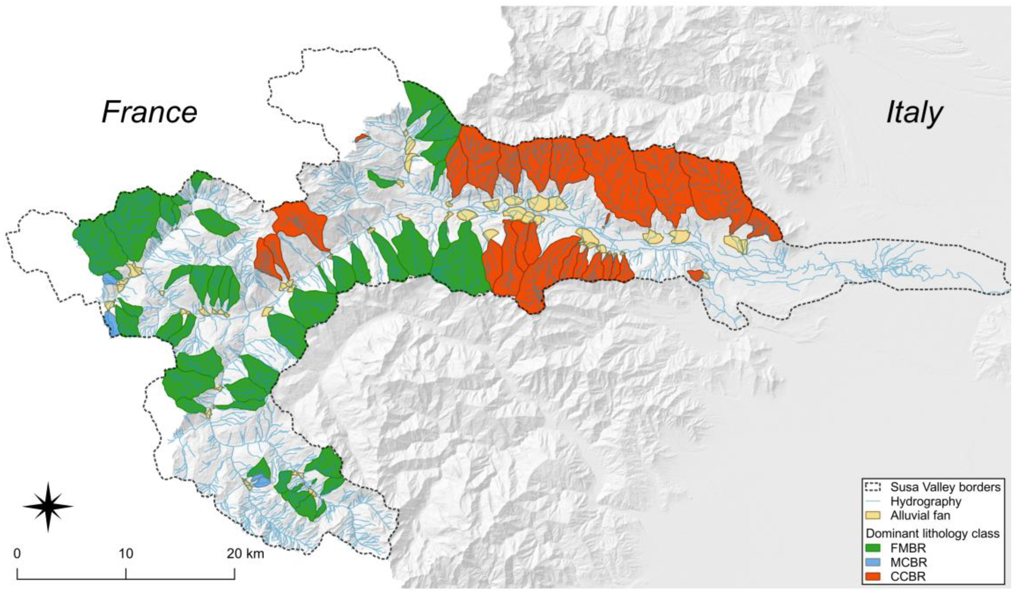
Study Area
2. Materials and Methods
2.1. Historical Recorded SGF and SFF Events
2.2. Catchment and Process Classification Method
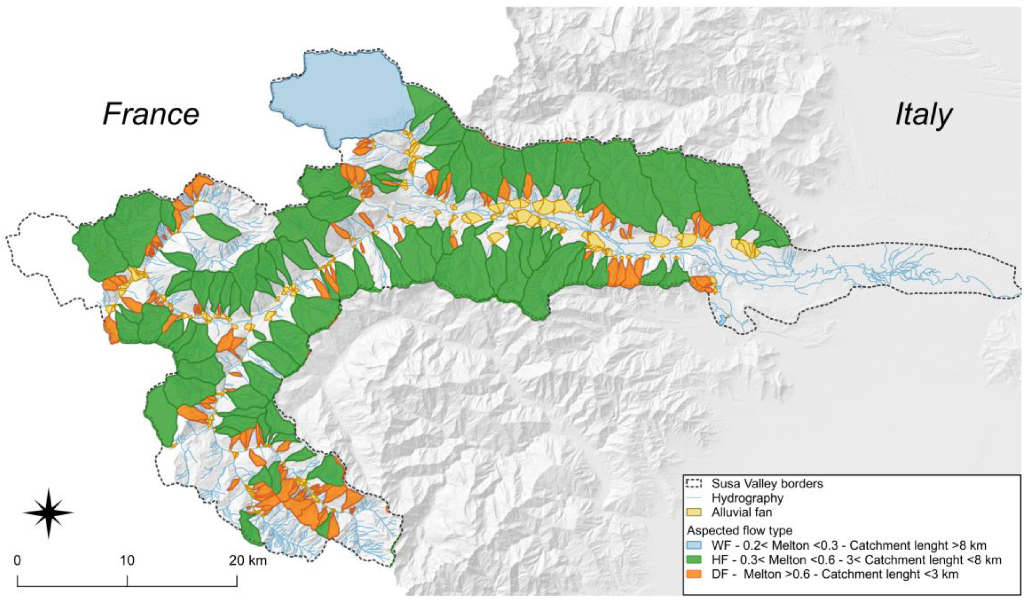
2.2.1. Catchments’ Classification by Morphometry
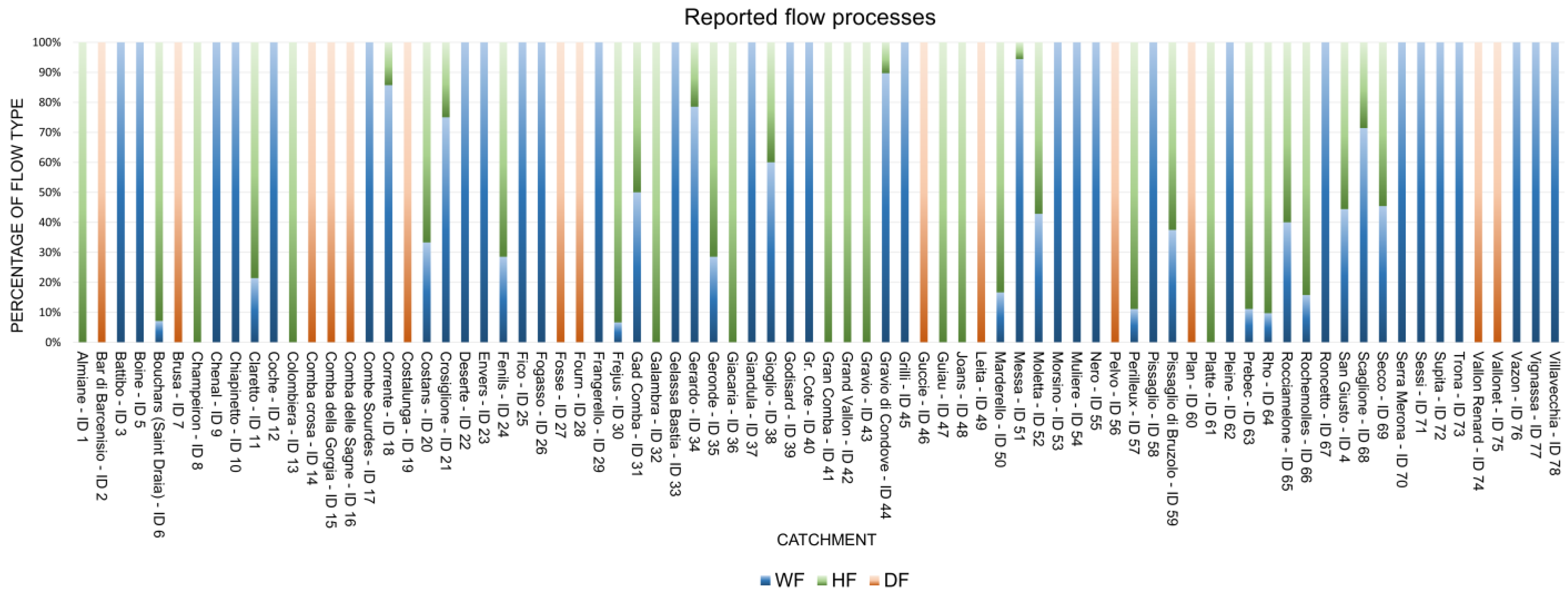
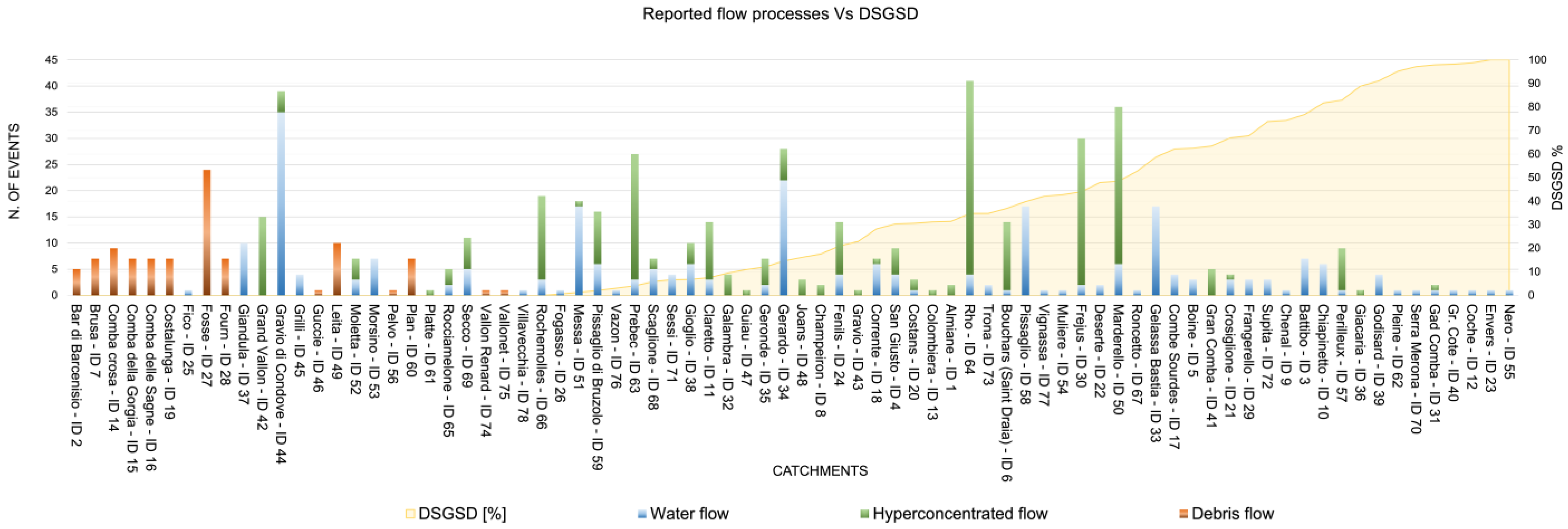
- Water flows (WFs) characterized by low sediment concentration (0.4–20%), transported via bedloading in a flow mixture displaying Newtonian behavior (SFF);
- Hyperconcentrated flows (HFs), represented by torrential mass-transport with moderate sediment concentration (>20–47%) in a flow mixture exhibiting either Newtonian or non-Newtonian behavior. An HF can therefore have the characteristics of either an SFF or an SGF depending on the concentration of the solid material being transported; typically, the transition from an SFF to an SGF occurs at a sediment concentration ≥ 30%;
- Debris flows (DFs), represented by SGF with high sediment concentration (>47–77%) in a flow mixture demonstrating non-Newtonian viscoplastic or collisional-frictional behavior related to the amount of fine sediment.
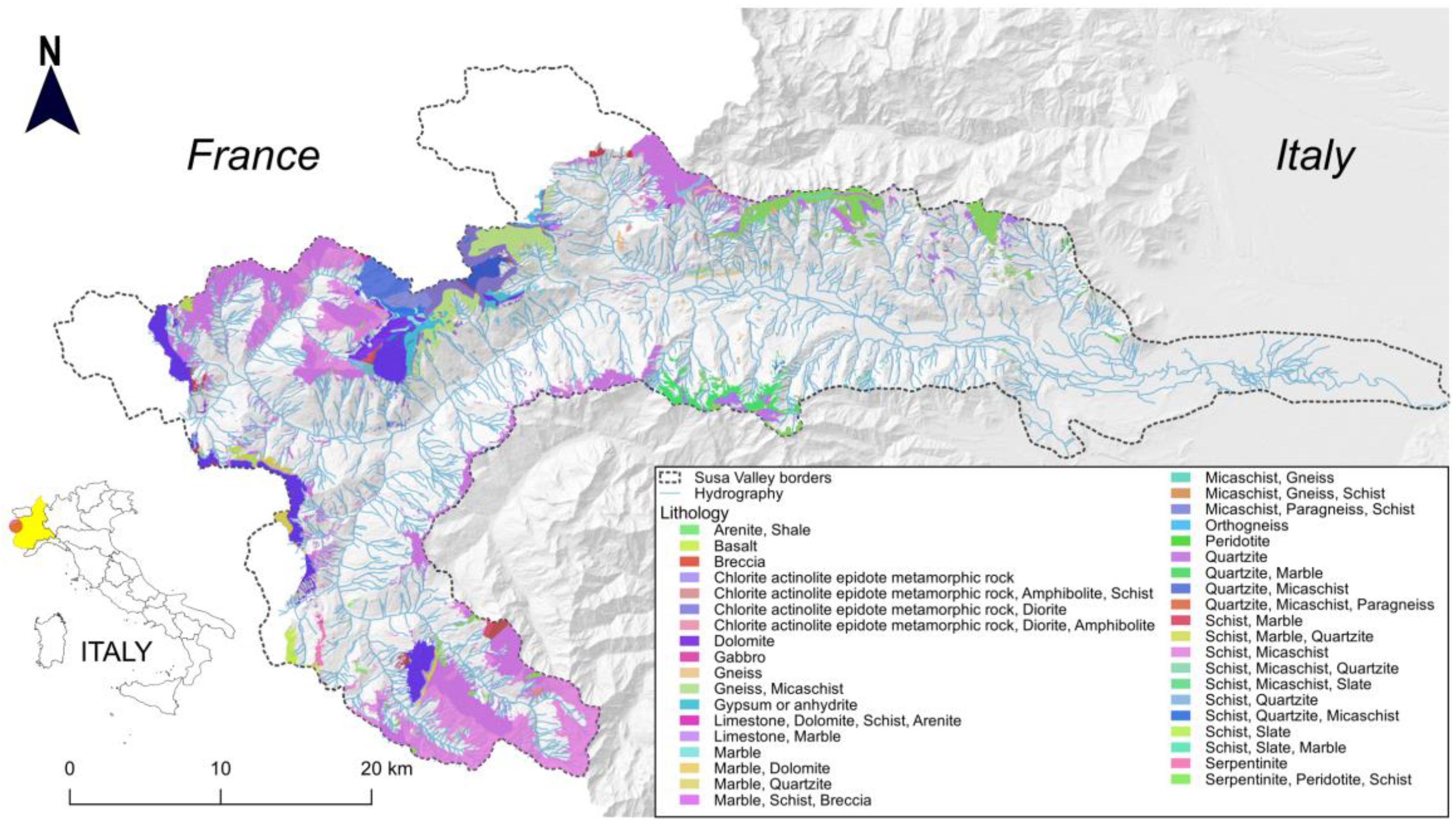
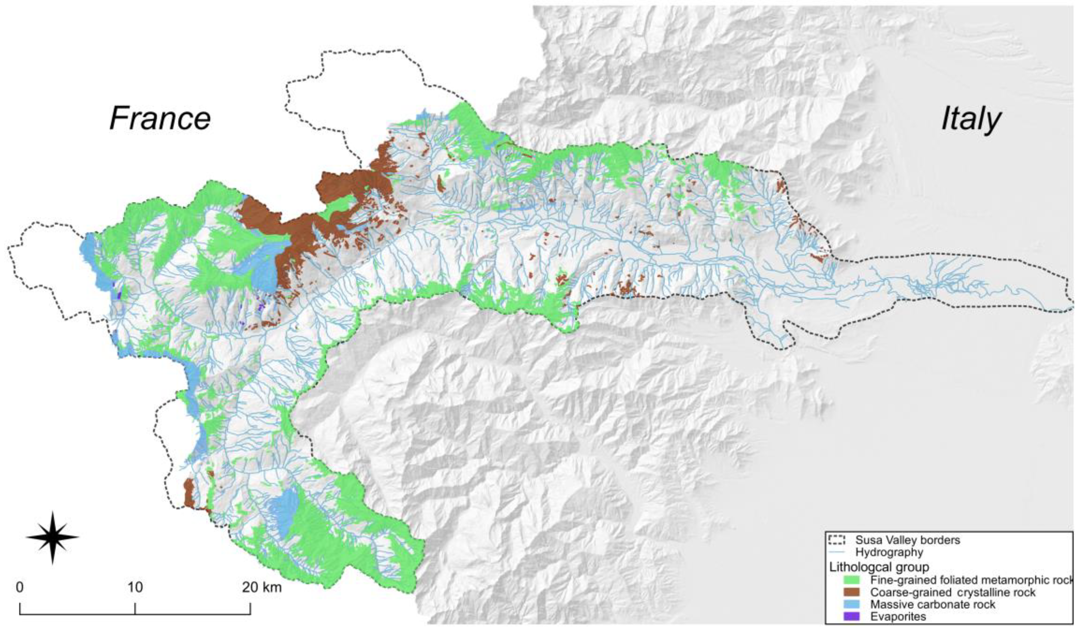
2.2.2. Determination of Catchments’ Dominant Bedrock’s Lithology
- Bedrock formed mainly by fine-grained schistose metamorphic rocks (FMBR), such as calc-schists, shales, slates, green schists, phyllites, etc.
- Bedrock formed mainly by massive or coarsely stratified carbonate rocks (MCBR), such as limestone, dolostones, marbles, cemented carbonate breccias and conglomerates, etc.
- Bedrock formed mainly by coarse-grained or massive crystalline rocks (CCBR), such as granitoids, gneiss, quartzites, eclogites, migmatites, peridotites, etc.
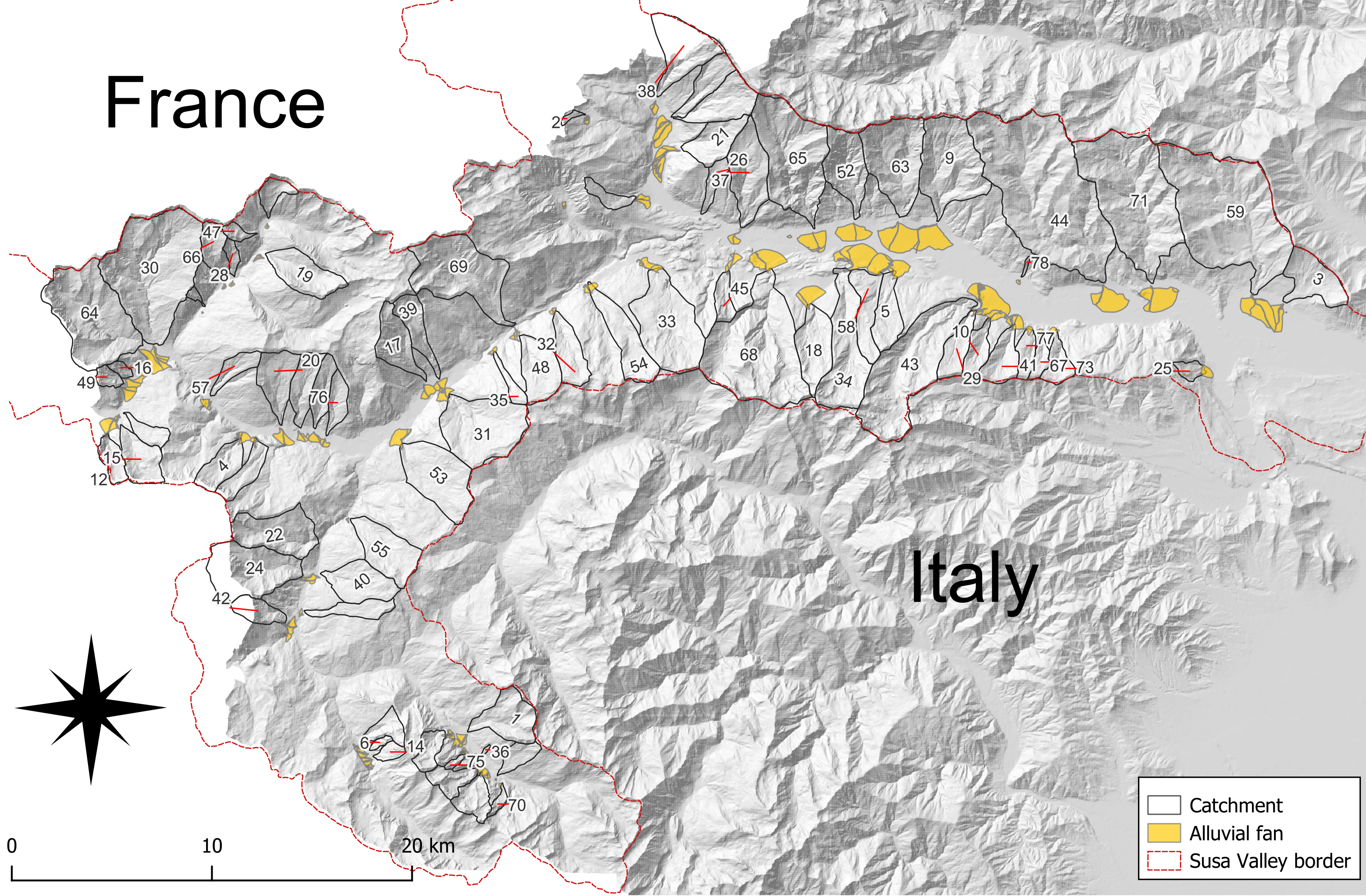
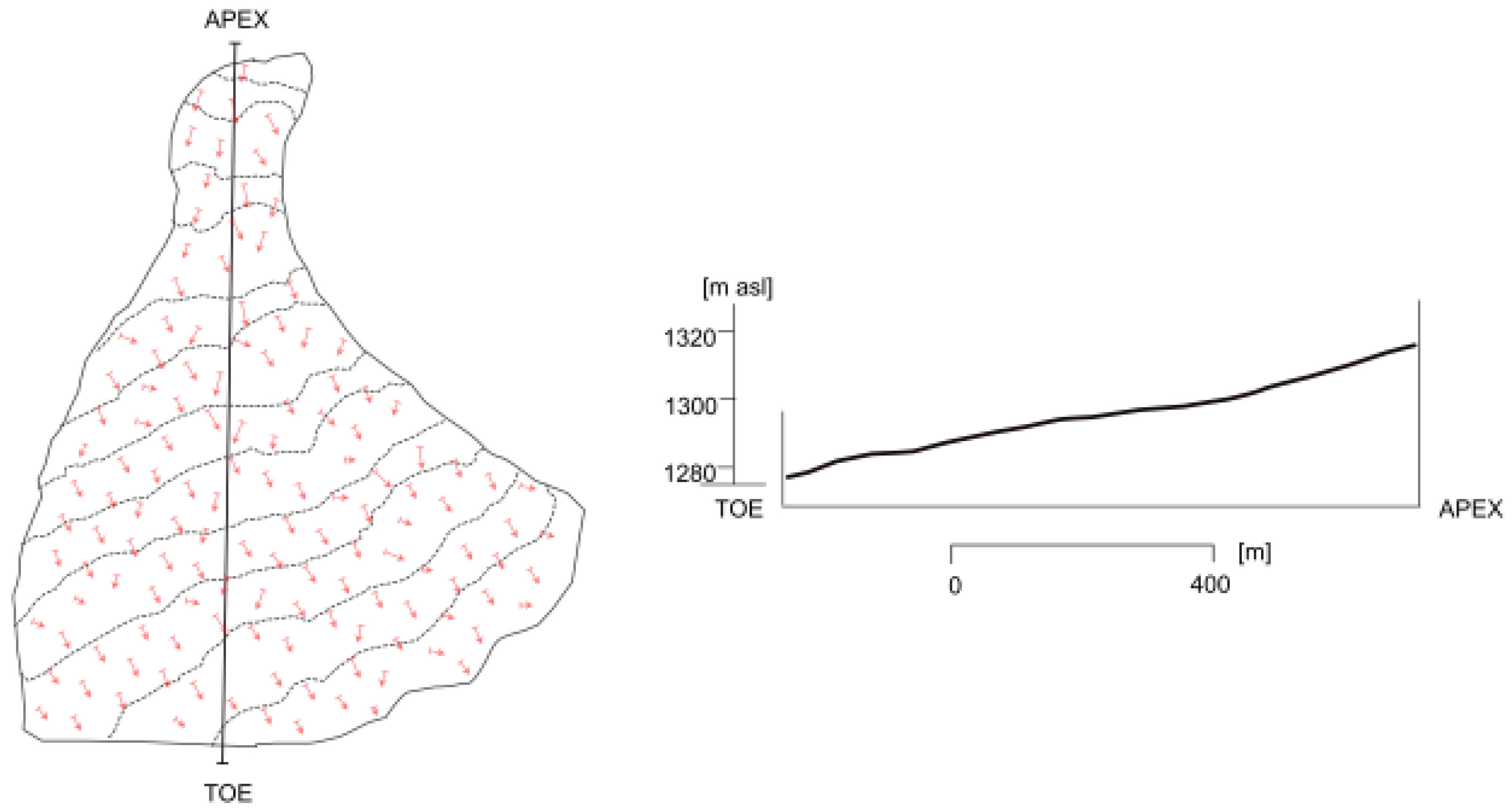
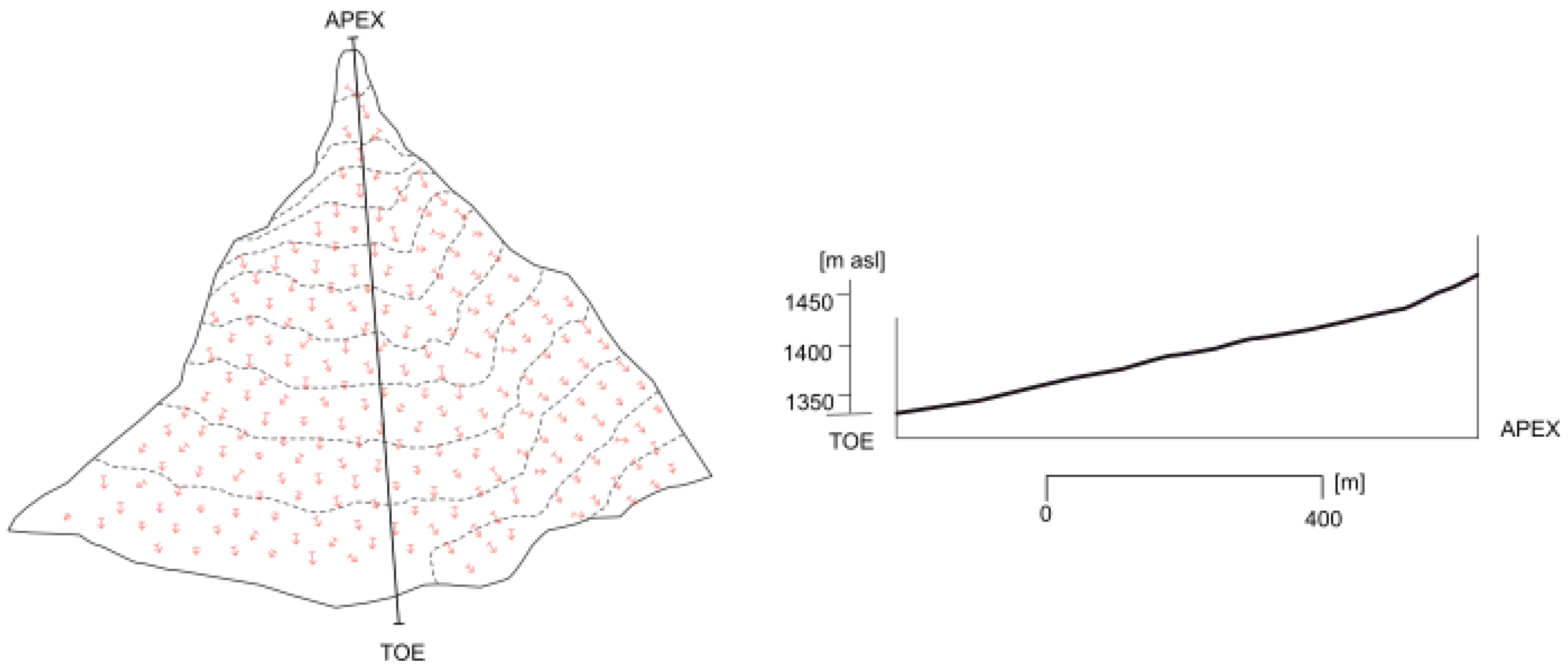
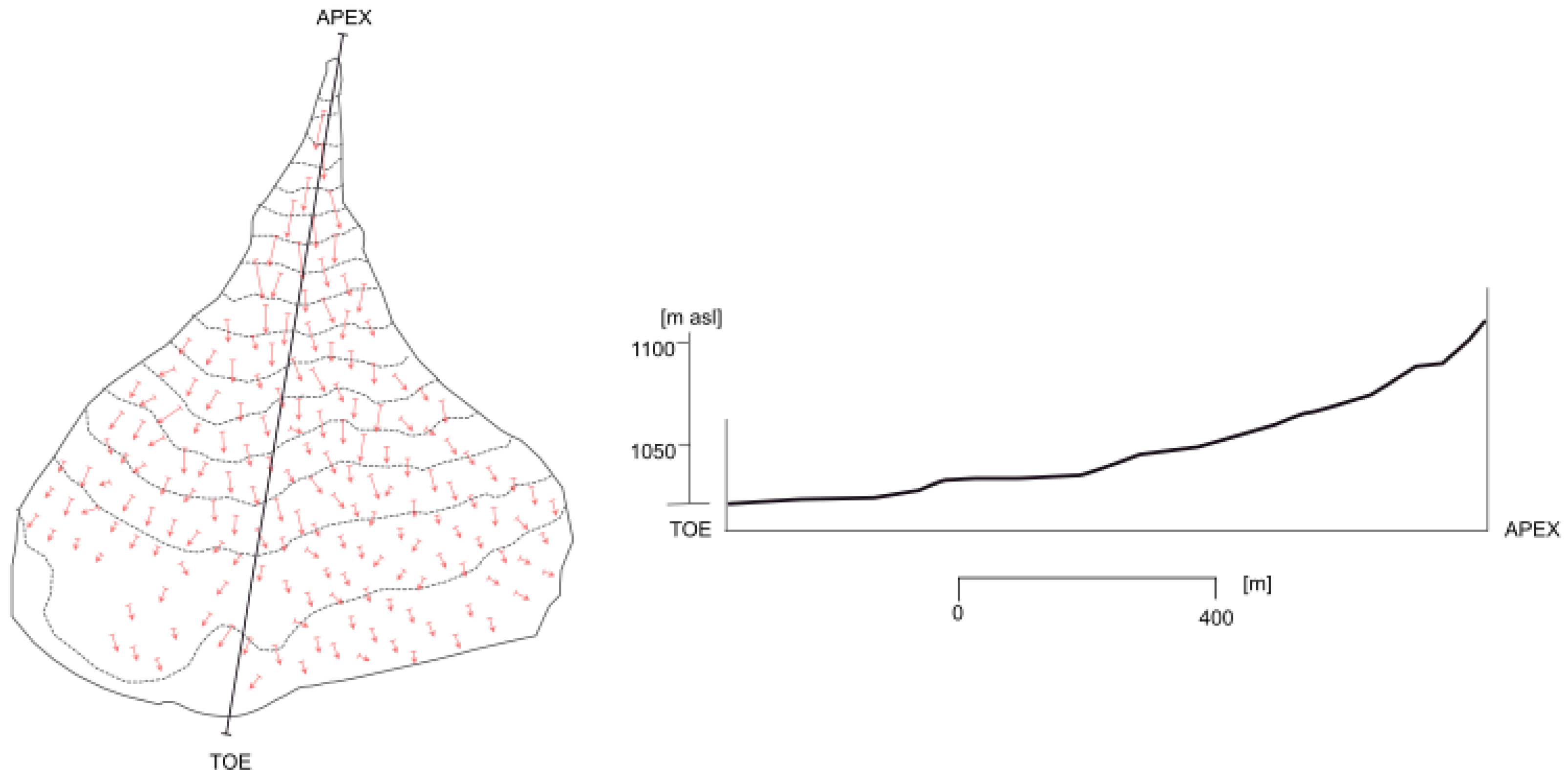
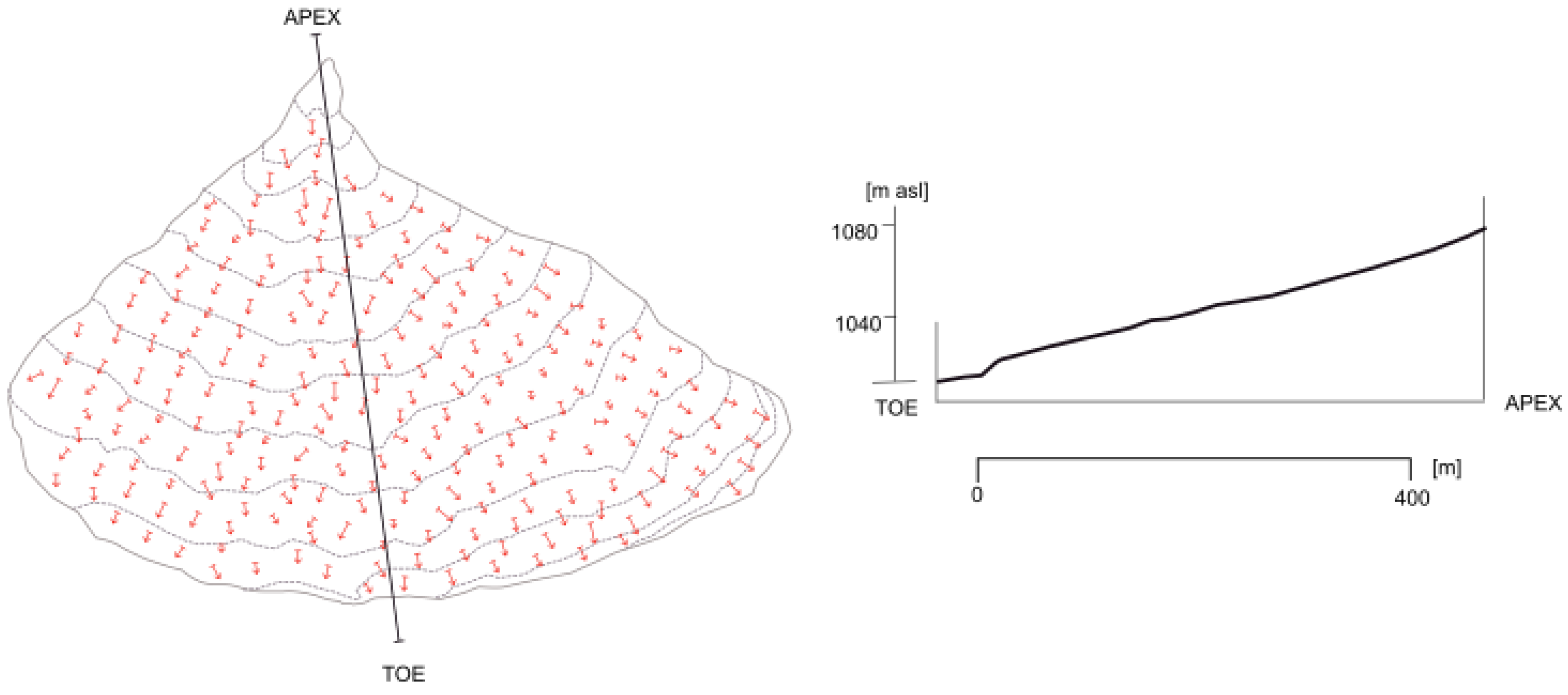
2.2.3. Characterization of Alluvial Fans
- Shape and area, determined by the identification of alluvial fans’ boundary by photogrammetric analysis in GIS environment and verified by field survey.
- Morphometry, obtaining the slope (mean and local distribution) of the alluvial fan depositional upper surface by processing the regional DTM 10 m.
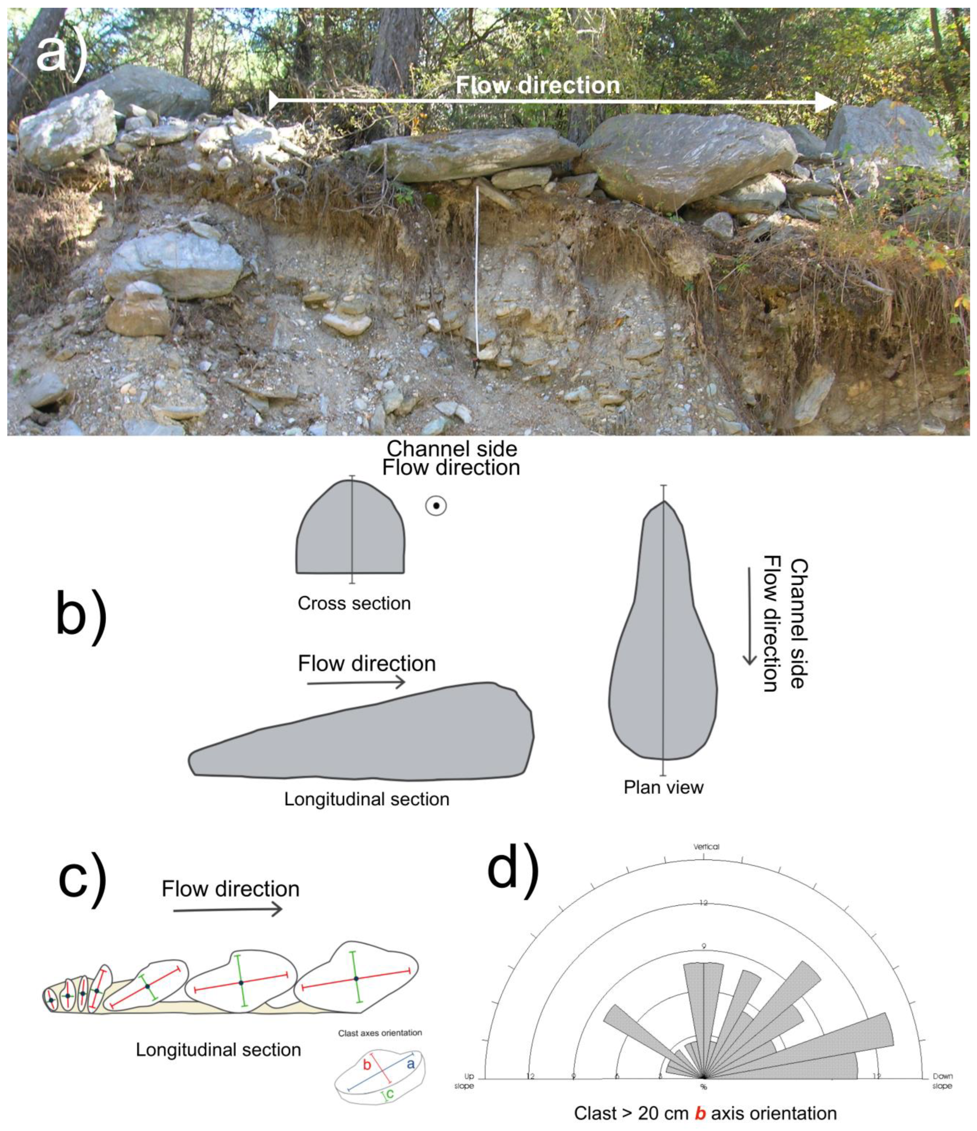
- Sedimentological characteristics such as clast-size distribution, deposits’ structure and texture, matrix abundance and grain size acquired by field surveys and laboratory analyses.
2.2.4. Characterization of SGF Deposits
3. Results
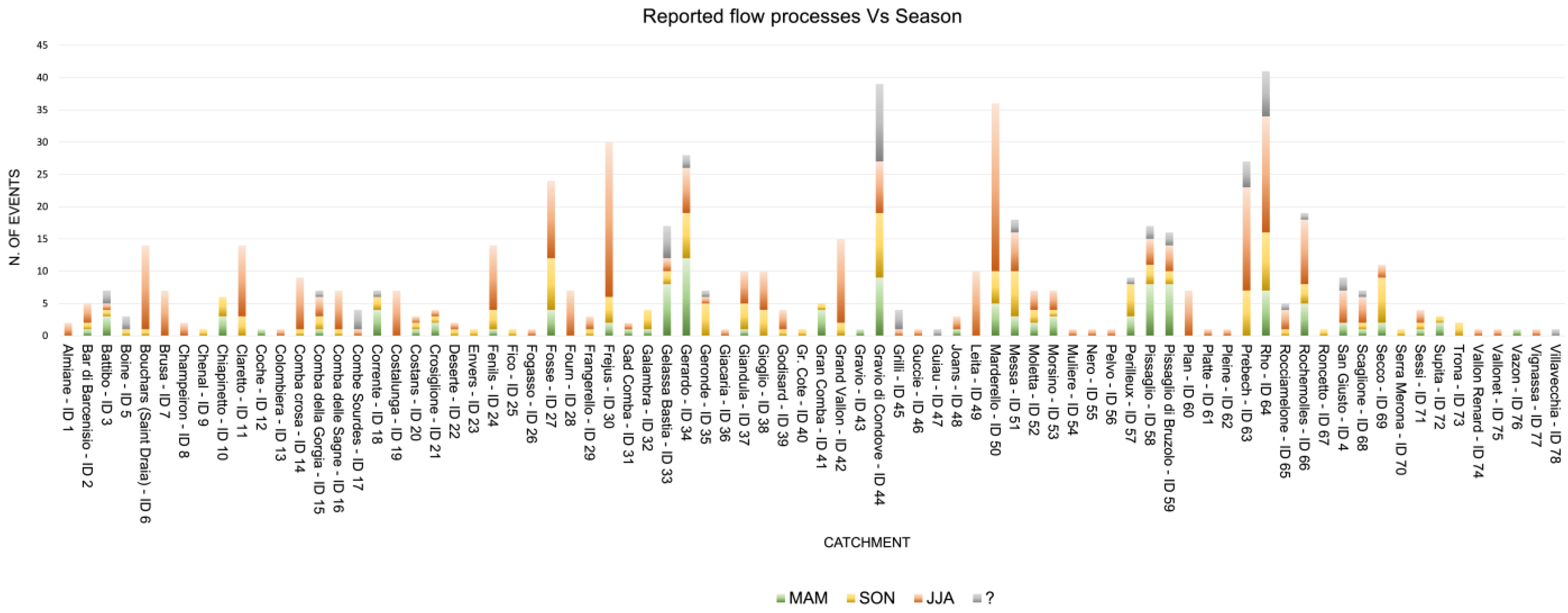
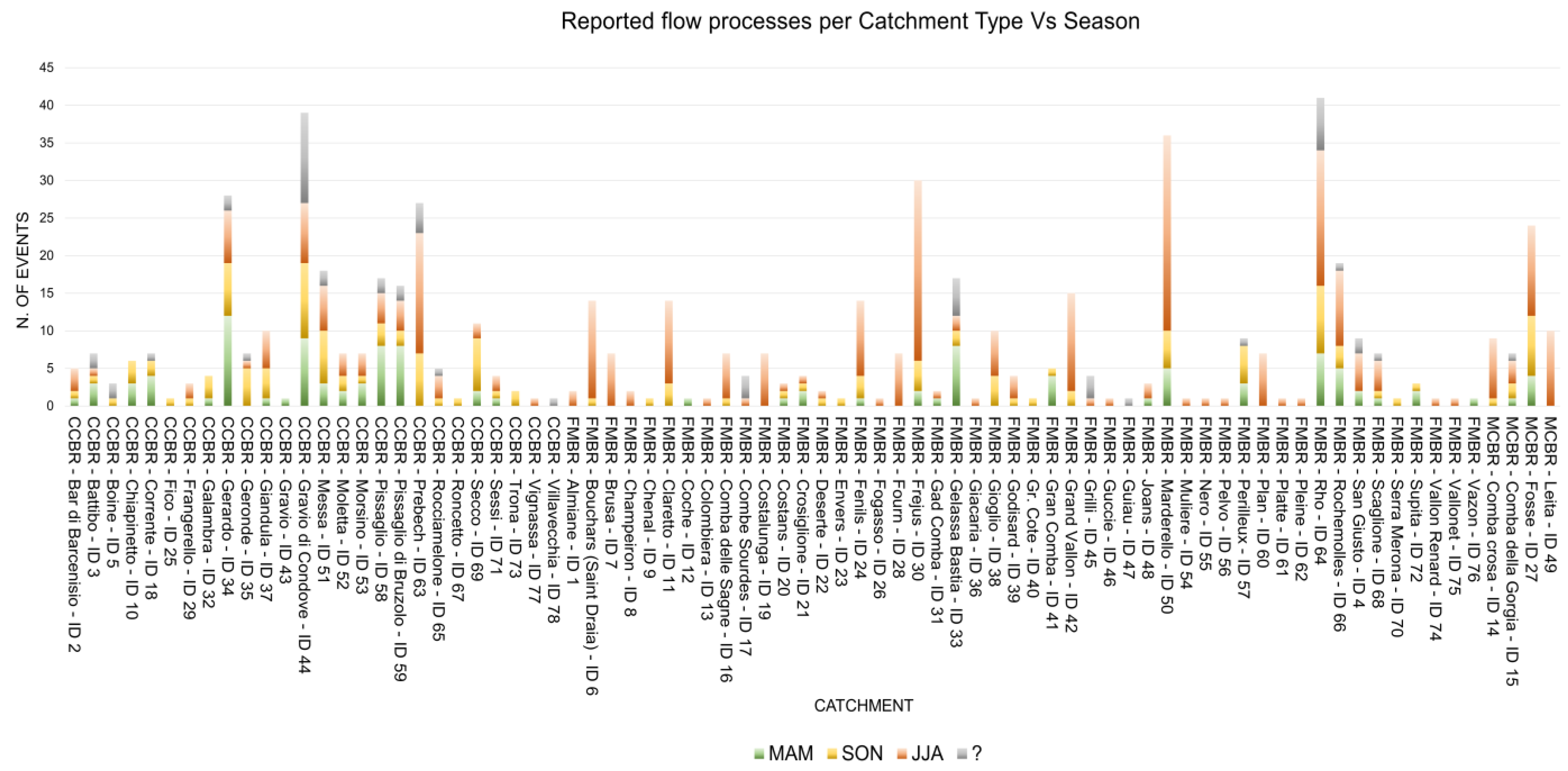
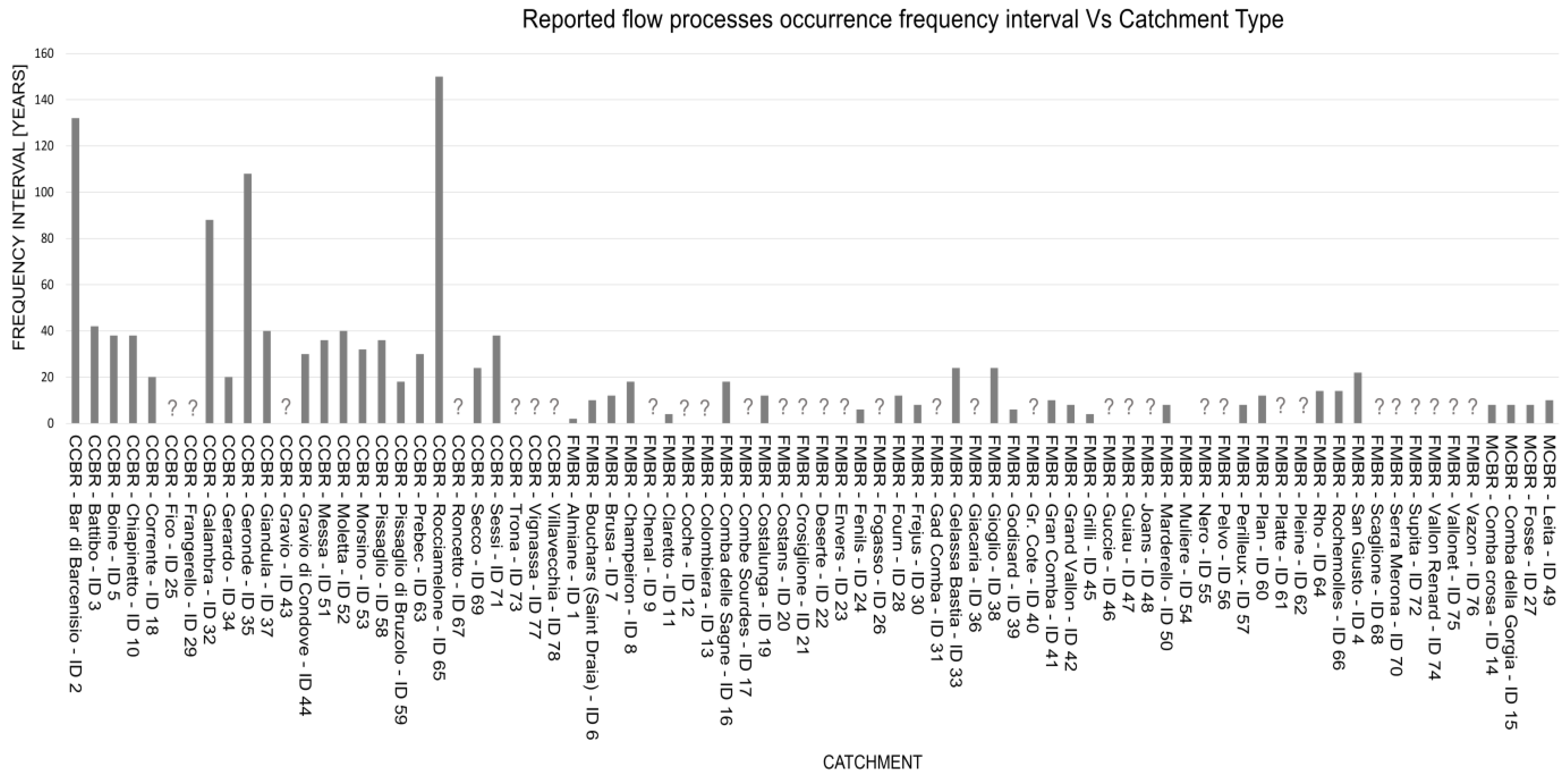
3.1. Historical SGF/SFF Event Behavior
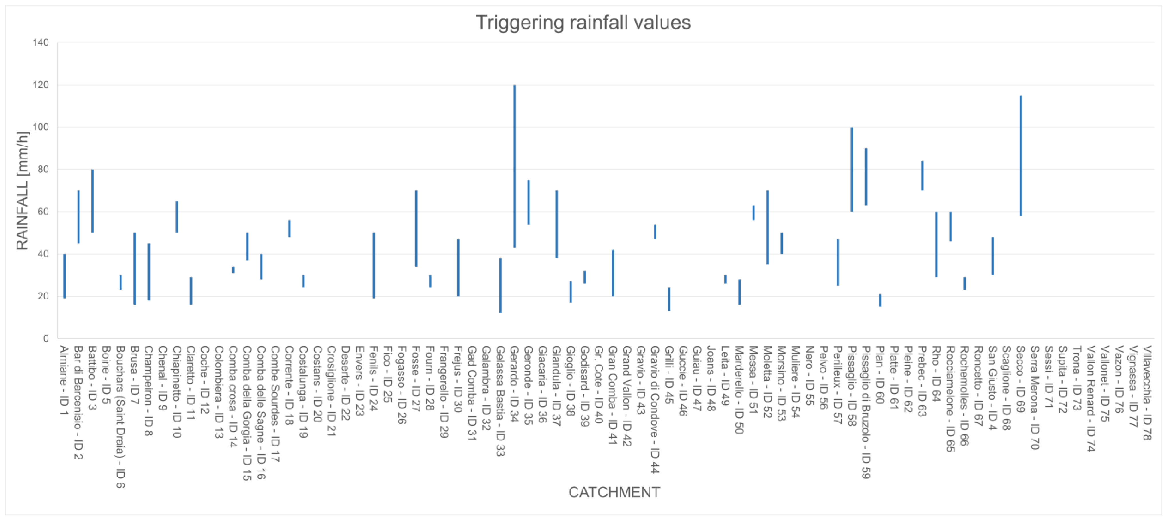
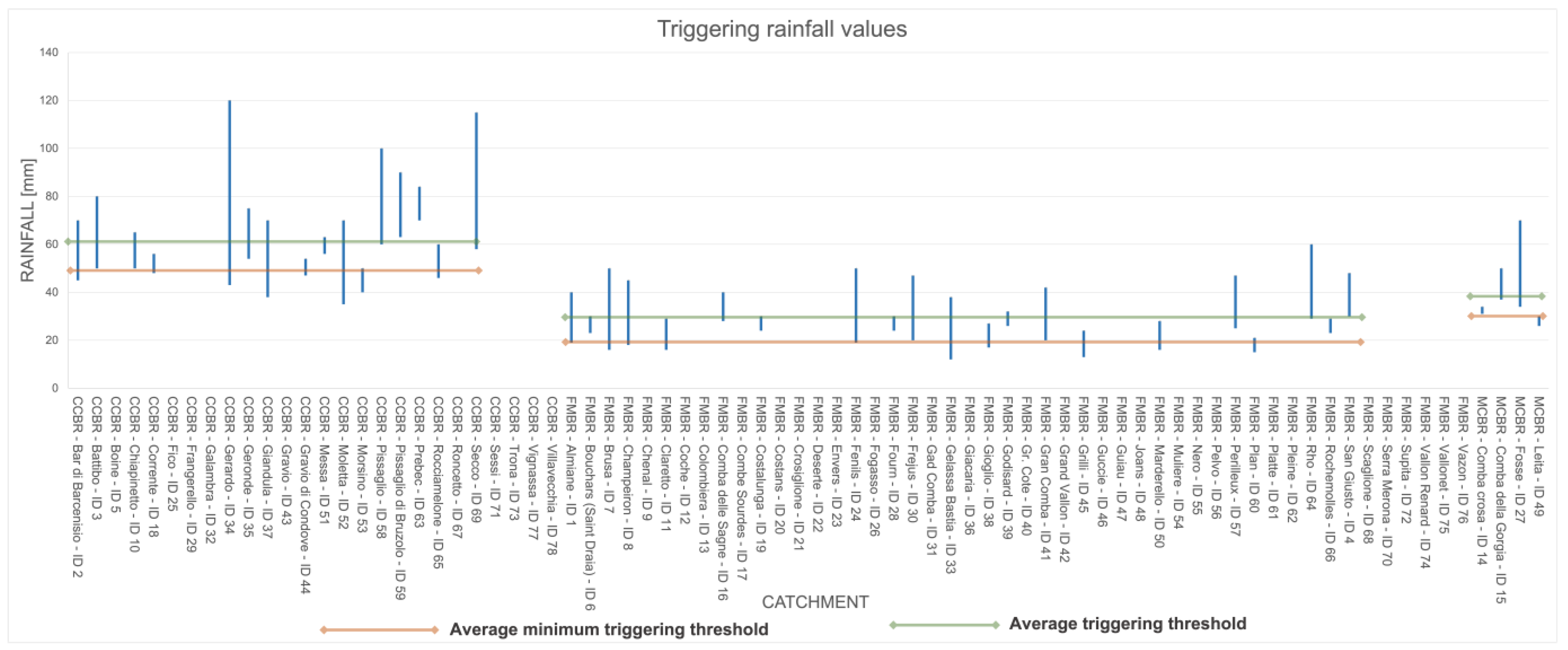
Rainfall-Triggering Thresholds
- Catchments where SGFs/SFFs are caused by rainfall every rainy season with higher incidence in summer (JJA) because of the higher frequency of rainstorms with intensity from moderate to very high, defining a minimum critical rainfall value from 20 to 30 mm/h (resulting from weather radar observations);
- Catchments where SGFs/SFFs are caused mainly by very high intensity rainfall peaks during extreme rainfall events that occur every rainy season with values ≥ 50 mm/h (resulting from weather radar observations).
3.2. Catchments’ Lithological Characterization
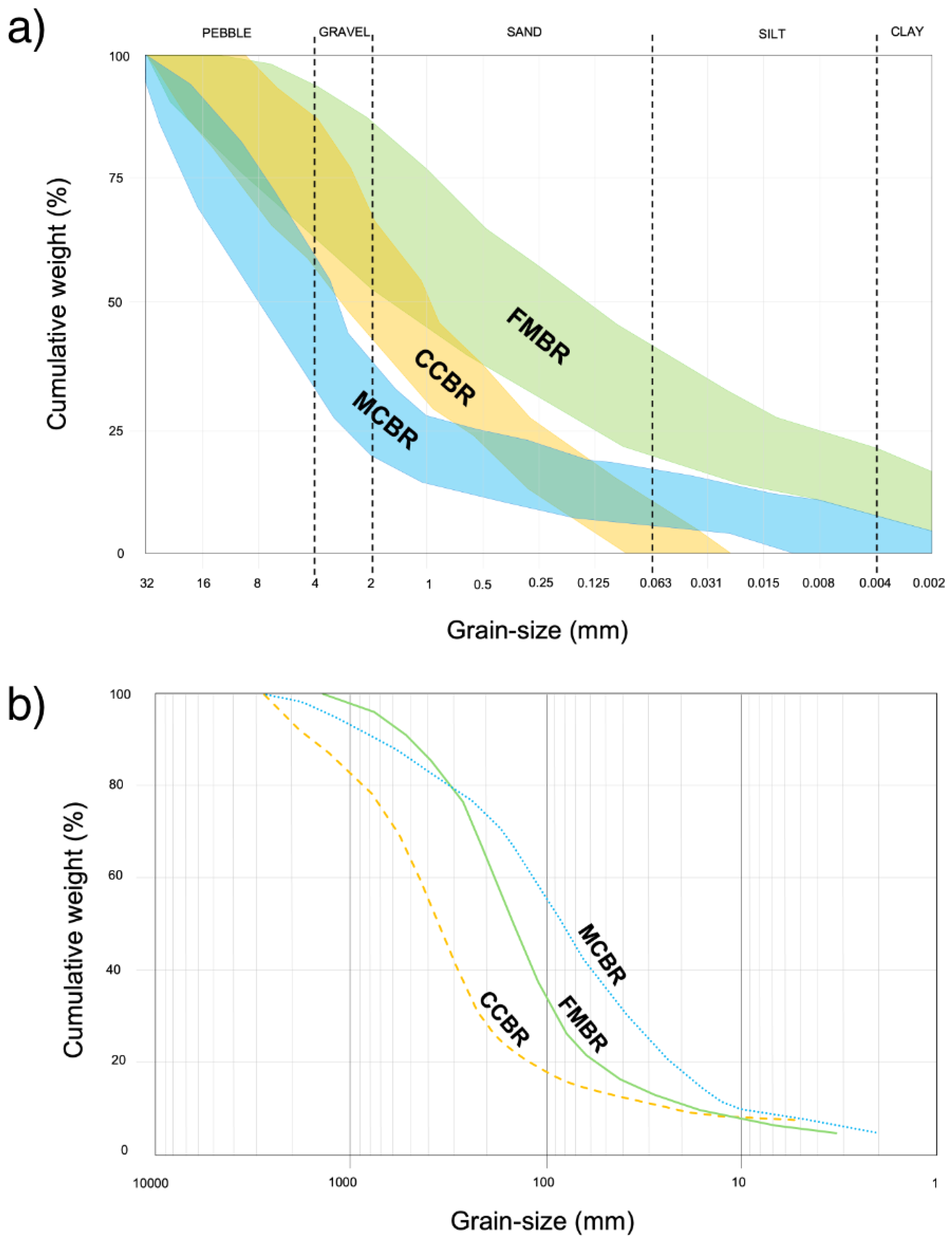
- Catchments having bedrock mainly formed by thin foliated metamorphic rocks (FMBR) characterized by poor geomechanical properties, producing abundant loose material with a high clay component (Figure 13) and being more predisposed to the accumulation of gravitational deposits (very susceptible to frequent small rock falls). The production of loose material resulting from the weathering of rock masses is constant and abundant, given the poor geomechanical characteristics of rocks. The coarse fraction of loose material is represented by the following:
- Rare boulder of 1–2 m3 with sphericity from prismoidal to sub-prismoidal and rarely spherical and roundness from angular to very angular;
- Common blocks of 0.50–0.70 m3 with sphericity from prismoidal to sub-discoidal and roundness from angular to very angular;
- Abundant cobbles/pebbles with sphericity from prismoidal to discoidal and roundness from angular to very angular;
- Very abundant gravels with sphericity from prismoidal to discoidal and roundness very angular.
- Catchments having bedrock mainly formed by massive carbonate rocks (MCBR) characterized by good geomechanical properties, producing moderate amounts of loose material (Figure 14) and non-negligible quantities of clayey sediment (clayey silt as insoluble fraction in carbonate rocks). The production of loose material resulting from the weathering of rock masses is quite constant and moderately abundant, given the good geomechanical characteristics of rocks. The coarse fraction of loose material is represented by the following:
- Common boulders of 1–3 m3 with sphericity from spherical to sub-discoidal and rarely sub-prismoidal and roundness from sub-angular to angular;
- Abundant blocks of 0.50–0.80 m3 with sphericity from spherical to sub-discoidal and rarely sub-prismoidal and roundness from angular to very angular;
- Very abundant cobbles/pebbles with sphericity from spherical to discoidal and roundness from angular to sub-angular;
- Very abundant gravels with sphericity from sub-prismoidal to discoidal and roundness angular.
- Catchments having bedrock mainly formed by coarse-grained crystalline rocks (CCBR) characterized by excellent geomechanical properties, producing smaller quantities of material in a comparable time period related to the other two types, in the form of loose material with abundant blocks and large boulders (Figure 15). Additionally, they are very poor producers of clay as a fine fraction. The coarse fraction of loose material is represented by the following:
- Rare mega-boulders of 15–20 m3 with sphericity from sub-discoidal to spherical and rarely sub-prismoidal and roundness from sub-angular to sub-rounded;
- Common boulders of 2–10 m3 with sphericity from sub-discoidal to spherical and rarely sub-prismoidal and roundness from sub-angular to sub-rounded;
- Abundant blocks of 0.50–1 m3 with sphericity from spherical to sub-discoidal and rarely sub-prismoidal and roundness from sub-angular to sub-rounded;
- Very abundant cobbles/pebbles with sphericity from spherical to sub-discoidal and roundness from angular to sub-angular;
- Very abundant gravels with sphericity from sub-prismoidal to sub-discoidal and roundness from angular to very angular.
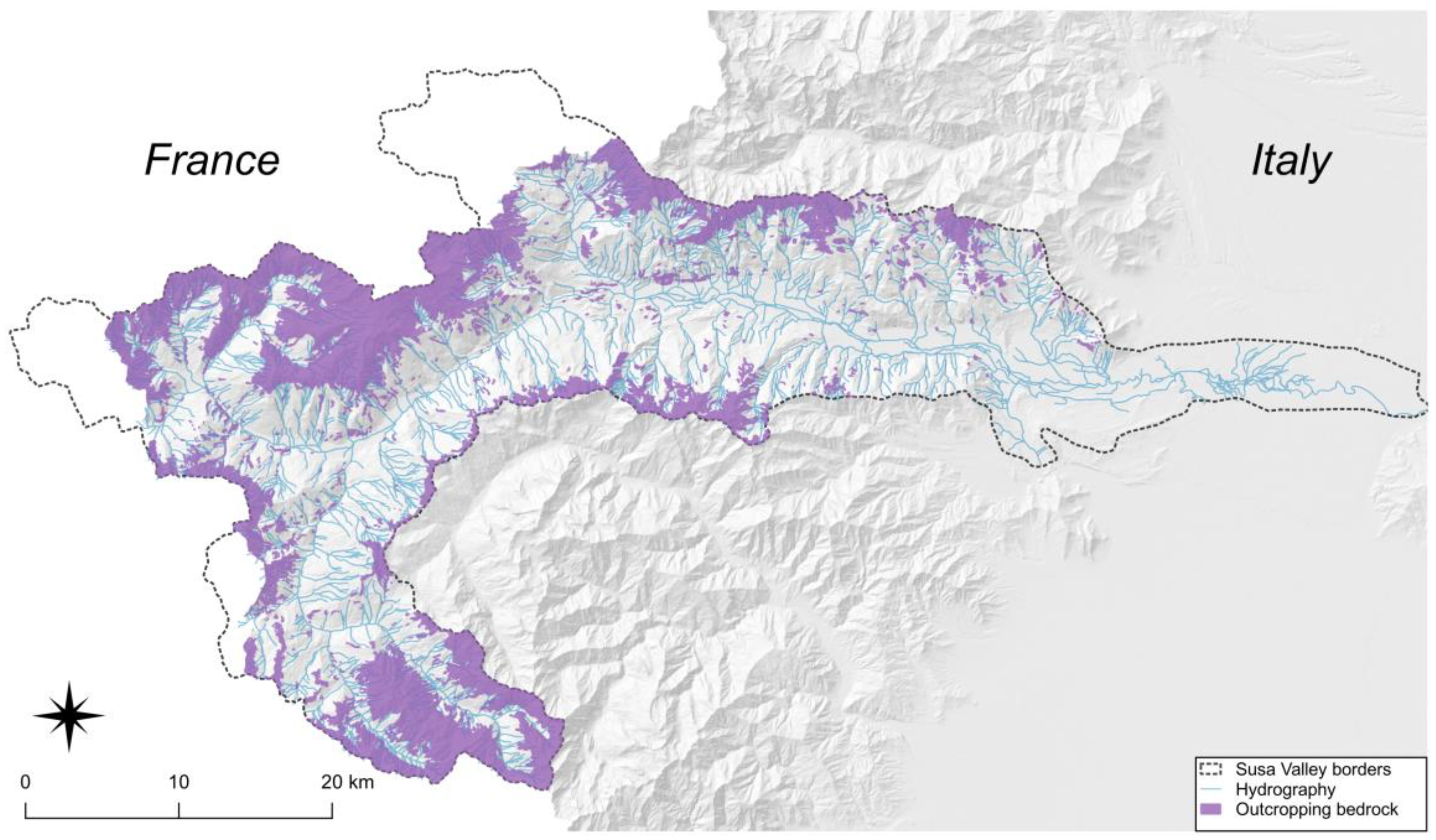
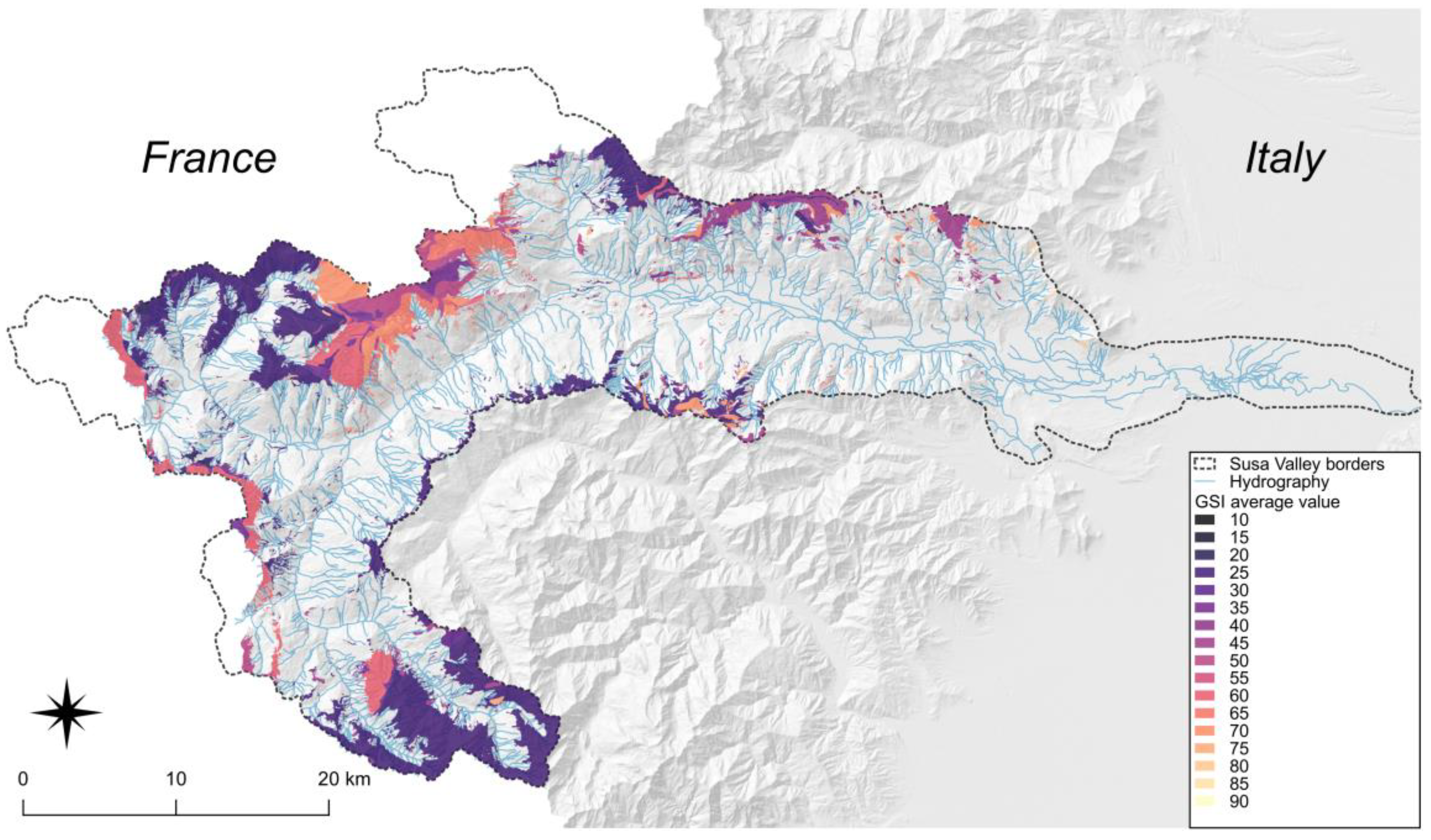
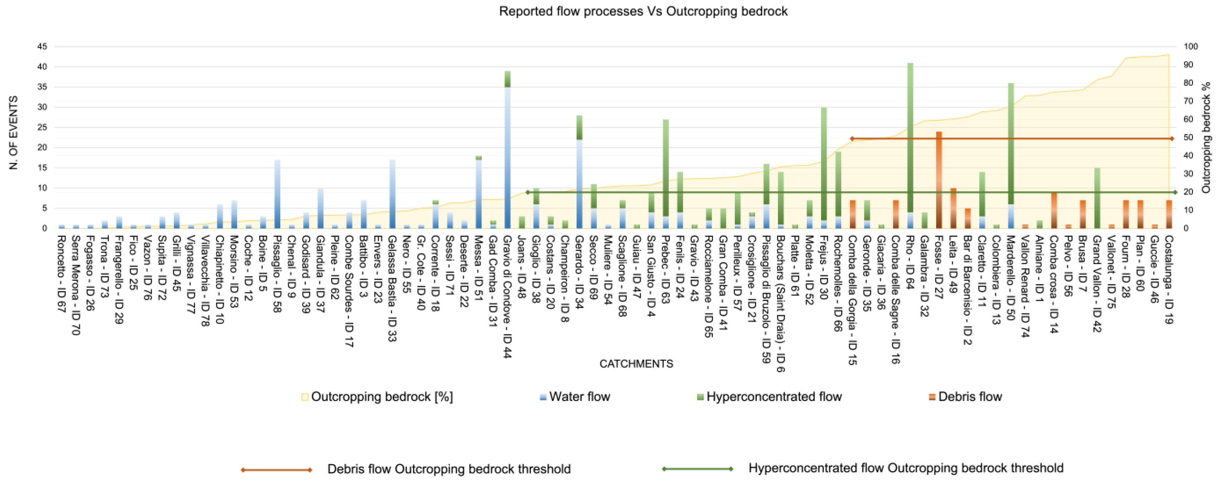
3.3. Morphometric Classification and Outcropping Bedrock Percentage
3.4. Alluvial Fan Caractherization
3.5. Deposit Description
4. Discussion
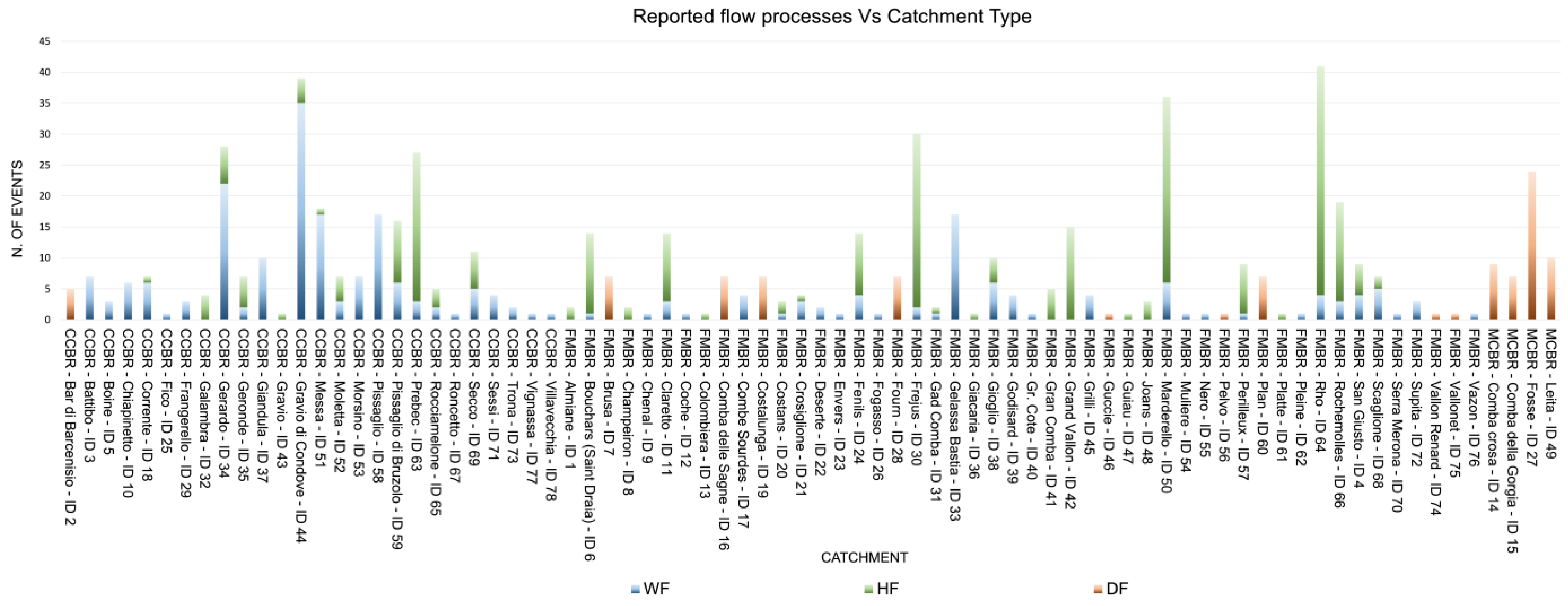
- FMBR catchments show 12% DFs, 61% HFs and 27% of WFs for a total of 326 flow events;
- MCBR catchments show 100% DFs for a total of 50 flow events;
- CCBR catchments show 2% of DFs, 29% HFs and 69% of WFs for a total of 238 flow events.
5. Conclusions
Funding
Data Availability Statement
Acknowledgments
Conflicts of Interest
References
- Campbell, R.H. Soil slips, debris flows, and rainstorms in the Santa Monica Mountains and vicinity, southern California. In US Geological Survey Professional Paper 851; U.S. Government Printing Office: Washington, DC, USA, 1975; p. 51. [Google Scholar]
- Caine, N. The rainfall intensity-duration control of shallow landslides and debris flow. Geogr. Ann. Ser. A Phys. Geogr. 1980, 62A, 23–27. [Google Scholar]
- Govi, M.; Sorzana, P.F. Landslide susceptibility as a function of critical rainfall amount in Piedmont basin (Northwestern Italy). Stud. Geomorph. Carpatho-Balc. 1980, 14, 43–61. [Google Scholar]
- Lin, P.S.; Lin, J.Y.; Huang, J.C.; Yang, M.D. Assessing debris-flow hazard in a watershed in Taiwan. Eng. Geol. 2002, 66, 295–313. [Google Scholar] [CrossRef]
- Jakob, M.; Hungr, O. Debris-Flow Hazards and Related Phenomena; Springer: Berlin/Heidelberg, Germany, 2005; pp. 1–538. [Google Scholar]
- Takahashi, T. Debris Flow Mechanics, Prediction and Countermeasures, 1st ed.; Taylor & Francis: London, UK, 2007; p. 448. [Google Scholar] [CrossRef]
- Hürlimann, M.; Rickenmann, D.; Medina, V.; Bateman, A. Evaluation of approaches to calculate debris-flow parameters for hazard assessment. Eng. Geol. 2008, 102, 152–163. [Google Scholar] [CrossRef]
- Ballesteros Cánovas, J.A.; Stoffel, M.; Corona, C.; Schraml, K.; Gobiet, A.; Tani, S.; Sinabell, F.; Fuchs, S.; Kaitna, R. Debris-flow risk analysis in a managed torrent based on a stochastic life-cycle performance. Sci. Total Environ. 2016, 557–558, 142–153. [Google Scholar] [CrossRef] [PubMed]
- Rogelis, M.C.; Werner, M. Regional debris flow susceptibility analysis in mountainous peri-urban areas through morphometric and land cover indicators. Nat. Hazards Earth Syst. Sci. 2014, 14, 3043–3064. [Google Scholar] [CrossRef]
- Hübl, J.; Fiebiger, G. Debris flow mitigation measures. In Debris Flow Hazards and Related Phenomena; Jakob, M., Hungr, O., Eds.; Springer: Chichester, UK, 2005; pp. 445–487. [Google Scholar]
- Itakura, Y.; Inaba, H.; Sawada, T. A debris-flow monitoring devices and methods bibliography. Nat. Hazards Earth Syst. Sci. 2005, 5, 971–977. [Google Scholar] [CrossRef]
- Holub, M.; Fuchs, S. Benefits of local structural protection to mitigate torrent-related hazards. WIT Trans. Inf. Commun. 2008, 39, 401–411. [Google Scholar]
- Bernard, M.; Barbini, M.; Boreggio, M.; Biasuzzi, K.; Gregoretti, C. Deposition areas: An effective solution for the reduction of the sediment volume transported by stony debris flows on the high-sloping reach of channels incising fans and debris cones. Earth Surf. Process. Landf. 2023, 49, 0197-9337. [Google Scholar] [CrossRef]
- Moscariello, A.; Marchi, L.; Maraga, F.; Mortara, G. Alluvial fans in the Alps: Sedimentary facies and processes. Spec. Publs. Int. Ass. Sediment. 2002, 32, 141–166. [Google Scholar]
- Tiranti, D.; Bonetto, S.; Mandrone, G. Quantitative basin characterization to refine debris-flow triggering criteria and processes: An example from the Italian Western Alps. Landslides 2008, 5, 45–57. [Google Scholar] [CrossRef]
- Tiranti, D.; Cremonini, R.; Marco, F.; Gaeta, A.R.; Barbero, S. The DEFENSE (DEbris Flows triggEred by storms—Nowcasting SystEm): An early warning system for torrential processes by radar storm tracking using a Geographic Information System (GIS). Comput. Geosci. 2014, 70, 96–109. [Google Scholar] [CrossRef]
- Tiranti, D.; Deangeli, C. Modeling of debris flow depositional patterns according to the catchments and sediment source areas characteristics. Front. Earth Sci. 2015, 3, 8. [Google Scholar] [CrossRef]
- Tiranti, D.; Cremonini, R.; Asprea, I.; Marco, F. Driving Factors for Torrential Mass-Movements Occurrence in the Western Alps. Front. Earth Sci. 2016, 4, 16. [Google Scholar] [CrossRef]
- Tiranti, D.; Cavalli, M.; Crema, S.; Zerbato, M.; Graziadei, M.; Barbero, S.; Cremonini, R.; Silvestro, C.; Bodrato, G.; Tresso, F. Semi-quantitative method for the assessment of debris supply from slopes to river in ungauged catchments. Sci. Total Environ. 2016, 554–555, 337–348. [Google Scholar] [CrossRef] [PubMed]
- Tiranti, D.; Crema, S.; Cavalli, M.; Deangeli, C. An Integrated Study to Evaluate Debris Flow Hazard in Alpine Environment. Front. Earth Sci. 2018, 6, 60. [Google Scholar] [CrossRef]
- Chen, H. The geomorphological comparison of two debris flows and their triggering mechanisms. Bull. Eng. Geol. Environ. 2000, 58, 297–308. [Google Scholar] [CrossRef]
- Glade, T. Linking debris-flow hazard assessments with geomorphology. Geomorphology 2005, 66, 189–213. [Google Scholar] [CrossRef]
- Stokes, M.; Mather, A.E. Controls on modern tributary-junction alluvial fan occurrence and morphology: High Atlas Mountains, Morocco. Geomorphology 2015, 248, 344–362. [Google Scholar] [CrossRef]
- Turconi, L.; Tropeano, D.; Savio, G.; Bono, B.; De, S.K.; Frasca, M.; Luino, F. Torrential Hazard Prevention in Alpine Small Basin through Historical, Empirical and Geomorphological Cross Analysis in NW Italy. Land 2022, 11, 699. [Google Scholar] [CrossRef]
- Palamakumbura, R.; Finlayson, A.; Ciurean, R.; Nedumpallile-Vasu, N.; Freeborough, K.; Dashwood, C. Geological and geomorphological influences on a recent debris flow event in the Ice-scoured Mountain Quaternary domain, western Scotland. Proc. Geol. Assoc. 2021, 132, 456–468. [Google Scholar] [CrossRef]
- Shuang, L.; Li, W.; Kaiheng, H. Topographical and geological variation of effective rainfall for debris-flow occurrence from a large-scale perspective. Geomorphology 2020, 358, 107134. [Google Scholar] [CrossRef]
- Zhuoya, L.; Yi, W.; Xianyin, M.; Qianyong, L.; Kuisen, Z.; Ming, Z. Faults and stratigraphic boundaries control evolution of the huge debris flows along the Jinjiang River, China. Front. Earth Sci. 2023, 11, 1237404. [Google Scholar] [CrossRef]
- Kumar, A.; Sarkar, R. Debris Flow Susceptibility Evaluation—A Review. Iran J. Sci. Technol. Trans. Civ. Eng. 2023, 47, 1277–1292. [Google Scholar] [CrossRef]
- Deganutti, A.M.; Marchi, L.; Arattano, M. Rainfall and debris flow occurrence in the Moscardo basin (Italian Alps). In Debris Flow Hazards Mitigation-Mechanics, Prediction, and Assessment; Wieczorek, G.F., Naeser, N.D., Eds.; Balkema: Rotterdam, The Netherland, 2000; pp. 67–72. [Google Scholar]
- Jomelli, V.; Pech, V.P.; Chochillon, C.; Brunstein, D. Geomorphic variations of debris flows and recent climatic change in the French Alps. Clim. Chang. 2004, 64, 77–102. [Google Scholar] [CrossRef]
- Wieczorek, G.F.; Glade, T. Climatic factors influencing occurrence of debris flow. In Debris Flow Hazard and Related Phenomena; Jacob, M., Hungr, H., Eds.; Springer: Berlin/Heidelberg, Germany, 2005; pp. 325–352. [Google Scholar]
- Stoffel, M.; Tiranti, D.; Huggel, C. Climate change impacts on mass movements—Case studies from the European Alps. Sci. Total Environ. 2014, 493, 1255–1266. [Google Scholar] [CrossRef] [PubMed]
- Destro, E.; Marra, F.; Nikolopoulos, E.I.; Zoccatelli, D.; Creutin, J.D.; Borga, M. A Spatial estimation of debris flows-triggering rainfall and its dependence on rainfall return period. Geomorphology 2017, 278, 269–279. [Google Scholar] [CrossRef]
- Santia, P.M.; deWolfea, V.G.; Higginsa, J.D.; Cannon, S.H.; Gartner, J.E. Sources of debris flow material in burned areas. Geomorphology 2008, 96, 310–321. [Google Scholar] [CrossRef]
- Kean, J.W.; McGuire, L.A.; Rengers, F.K.; Smith, J.B.; Staley, D.M. Amplification of post-wildfire peak flow by debris. Geophys. Res. Lett. 2016, 43, 8545–8553. [Google Scholar] [CrossRef]
- Staley, D.M.; Kean, J.W.; Rengers, F.K. The recurrence interval of post- fire debris-flow generating rainfall in the southwestern United States. Geomorphology 2020, 370, 107392. [Google Scholar] [CrossRef]
- Tiranti, D.; Cremonini, R.; Sanmartino, D. Wildfires effect on debris flow occurrence in Italian Western Alps: Preliminary considerations to refine debris flow early warnings system criteria. Geosciences 2021, 11, 422. [Google Scholar] [CrossRef]
- Spyrou, M.; Petropoulos, E.; Karkani, A.; Saitis, G.; Margaritis, A.M. GIS-Based Assessment of Fire Effects on Flash Flood Hazard: The Case of the Summer 2021 Forest Fires in Greece. GeoHazards 2023, 4, 1–22. [Google Scholar] [CrossRef]
- Palacios, D.; Parrilla, G.; Zamorano, J.J. Paraglacial and postglacial debris flows on a Little Ice Age terminal moraine: Jamapa Glacier, Pico de Orizaba (Mexico). Geomorphology 1999, 28, 95–118. [Google Scholar] [CrossRef]
- Bardou, E.; Delaloye, R. Effects of ground freezing and snow avalanche deposits on debris flows in alpine environments. Nat. Hazards Earth Syst. Sci. 2004, 4, 519–530. [Google Scholar] [CrossRef]
- Breien, H.; De Blasio, F.V.; Elverhøi, A.; Høeg, K. Erosion and morphology of a debris flow caused by a glacial lake outburst flood, Western Norway. Landslides 2008, 5, 271–280. [Google Scholar] [CrossRef]
- Stoffel, M.; Bollschweiler, M.; Beniston, M. Rainfall characteristics for periglacial debris flows in the Swiss Alps: Past incidences–potential future evolutions. Clim. Chang. 2011, 105, 263–280. [Google Scholar] [CrossRef]
- Stoffel, M.; Graf, C. Debris-flow activity from high-elevation, periglacial environments. In The High-Mountain Cryosphere; Huggel, C., Carey, M., Clague, J.J., Kääb, A., Eds.; Cambridge University Press: Cambridge, UK, 2015. [Google Scholar] [CrossRef]
- Chen, N.S.; Hu, G.S.; Deng, M.F.; Yang, C.L.; Zhou, W.; Deng, J.H. Impact of earthquake on debris flows—A case study on the Wenchuan earthquake. J. Earthq. Tsunami 2011, 5, 493–508. [Google Scholar] [CrossRef]
- Li, S.H.D.; Ren, X.S.; Yue, S.Y.; Xu, H.P. Earthquake and debris flows activities. Res. Soil Water Conserv. 2001, 8, 26–27. [Google Scholar]
- Chen, M.; Chang, M.; Xu, Q.; Tang, C.; Dong, X.; Li, L. Identifying potential debris flow hazards after the 2022 Mw 6.8 Luding earthquake in southwestern China. Bull. Eng. Geol. Environ. 2024, 83, 241. [Google Scholar] [CrossRef]
- Polino, R.; Dela Pierre, F.; Fioraso, G.; Giardino, M.; Gattiglio, M. Foglio 132-152-153 “Bardonecchia” Carta Geologica d’Italia. Scala 1:50000; Servizio Geologico D’italia: Romo, Italy, 2002. [Google Scholar]
- Piana, F.; Fioraso, G.; Irace, A.; Mosca, P.; d’Atri, A.; Barale, L.; Falletti, P.; Monegato, G.; Morelli, M.; Tallone, S.; et al. Geology of Piemonte region (NW Italy, Alps–Apennines interference zone). J. Maps 2017, 13, 395–405. [Google Scholar] [CrossRef]
- Fratianni, S.; Motta, L. Andamento climatico in alta Val Susa negli anni 1990–1999. In Studi Climatologici in Piemonte; Regione Piemonte, Ed.; Regione Piemonte: Turin, Italy, 2002. [Google Scholar]
- Wilford, D.J.; Sakals, M.E.; Innes, J.L.; Sidle, R.C.; Bergerud, W.A. Recognition of debris flow, debris flood and flood hazard through watershed morphometrics. Landslides 2004, 1, 61–66. [Google Scholar] [CrossRef]
- Pierson, T.C.; Costa, J.E. A rheologic classification of subaerial sediment–water flows. Geol. Soc. Am. Rev. Eng. Geol. 1987, 7, 1–12. [Google Scholar]
- Costa, J.E. Rheologic, geomorphic, and sedimentologic differentiation of water floods, hyperconcentrated flows, and debris flows. In Flood Geomorphology; Baker, V.R., Kochel, R.C., Patton, R.C., Eds.; John Wiley and Sons: New York, NY, USA, 1988; pp. 113–122. [Google Scholar]
- Lavigne, F.; Suwa, H. Contrasts between debris flows, hyperconcentrated flows and stream flows at channel of Mount Semeru, East Java, Indonesia. Geomorphology 2004, 61, 41–58. [Google Scholar] [CrossRef]
- Melton, M.A. An Analysis of the Relation Among Elements of Climate, Surface Properties and Geomorphology; Department of Geology, Columbia University: New York, NY, USA, 1957. [Google Scholar]
- Marinos, V.; Marinos, P.; Hoek, E. The geological strength index: Applications and limitations. Bull. Eng. Geol. Environ. 2005, 64, 55–65. [Google Scholar] [CrossRef]
- Vianello, D.; Vagnon, F.; Bonetto, S.; Mosca, P. Debris flow susceptibility mapping using the Rock Engineering System (RES) method: A case study. Landslides 2023, 20, 735–756. [Google Scholar] [CrossRef]
- Blair, T.C.; McPherson, J.G. Alluvial fans and their natural distinction from rivers based on morphology, hydraulic processes, sedimentary processes, and facies assemblages. J. Sediment. Res. 1994, A64, 450–489. [Google Scholar]
- Varnes, D.J. Slope movements types and processes. In Landslides: Analysis and Control; Schuster, R.L., Krizeck, R.J., Eds.; National Academy of Sciences: Washington, DC, USA, 1978; pp. 11–30. [Google Scholar]
- Paranunzio, R.; Laio, F.; Nigrelli, G.; Chiarle, M. A method to reveal climatic variables triggering slope failures at high elevation. Nat. Hazards 2015, 76, 1039–1061. [Google Scholar] [CrossRef]
- Miller, H.J. Tobler’s First Law and Spatial Analysis. Ann. Assoc. Am. Geogr. 2004, 94, 284–289. [Google Scholar] [CrossRef]
- Davini, P.; Bechini, R.; Cremonini, R.; Cassardo, C. Radar-based analysis of convective storms over Northwestern Italy. Atmosphere 2012, 3, 33–58. [Google Scholar] [CrossRef]
- Wolfgang, K.H.; Simar, L. Applied Multivariate Statistical Analysis, 5th ed.; Springer Nature: Cham, Switzerland, 2019; p. 558. [Google Scholar] [CrossRef]


| Area | Rainfall Value (mm/h) | Reference Return Period (years) |
|---|---|---|
| Susa Valley (Cottian Alps) | 20 | 5 |
| 30 | 20 | |
| 50 | 100 |
| Catchment Type | Mean Area (%) of Alluvial Fan Compared to the Area of the Feeding Catchment |
|---|---|
| FMBR | 20 |
| MCBR | 5 |
| CCBR | 10 |
| Time | Intensity | ||||
|---|---|---|---|---|---|
| Catchment Group | SGF/SFF Frequency | Rainfall Return Period * | SGF Relative Occurrence ** | SGF Intensity | Relative Hazard Degree |
| FMBR | Moderate (0.2) | Low (0.3) | Moderate (0.2) | Low/moderate (0.3) | Low (1.0) |
| CMBR | High (0.3) | Moderate (0.2) | High (0.3) | Moderate/high (0.4) | Moderate (1.2) |
| CCBR | Low (0.1) | High (0.1) | Moderate (0.2) | High/very high (1) | High (1.4) |
Disclaimer/Publisher’s Note: The statements, opinions and data contained in all publications are solely those of the individual author(s) and contributor(s) and not of MDPI and/or the editor(s). MDPI and/or the editor(s) disclaim responsibility for any injury to people or property resulting from any ideas, methods, instructions or products referred to in the content. |
© 2024 by the author. Licensee MDPI, Basel, Switzerland. This article is an open access article distributed under the terms and conditions of the Creative Commons Attribution (CC BY) license (https://creativecommons.org/licenses/by/4.0/).
Share and Cite
Tiranti, D. Alpine Catchments’ Hazard Related to Subaerial Sediment Gravity Flows Estimated on Dominant Lithology and Outcropping Bedrock Percentage. GeoHazards 2024, 5, 652-682. https://doi.org/10.3390/geohazards5030034
Tiranti D. Alpine Catchments’ Hazard Related to Subaerial Sediment Gravity Flows Estimated on Dominant Lithology and Outcropping Bedrock Percentage. GeoHazards. 2024; 5(3):652-682. https://doi.org/10.3390/geohazards5030034
Chicago/Turabian StyleTiranti, Davide. 2024. "Alpine Catchments’ Hazard Related to Subaerial Sediment Gravity Flows Estimated on Dominant Lithology and Outcropping Bedrock Percentage" GeoHazards 5, no. 3: 652-682. https://doi.org/10.3390/geohazards5030034
APA StyleTiranti, D. (2024). Alpine Catchments’ Hazard Related to Subaerial Sediment Gravity Flows Estimated on Dominant Lithology and Outcropping Bedrock Percentage. GeoHazards, 5(3), 652-682. https://doi.org/10.3390/geohazards5030034