Article

Landslide Occurrence Analysis in a Data-Scarce Region: The Northern Andes of Ecuador

1
Department of Chemistry & Geochemistry, Montana Technological University, Butte, MT 59701, USA
2
School of Earth Science, Energy and Environment, Grupo de Investigación en Clima y Procesos de Superficie (HYDROCLIMA), Yachay Tech University, Urcuquí 100115, Ecuador
*
Author to whom correspondence should be addressed.
GeoHazards 2026, 7(4), 108; https://doi.org/10.3390/geohazards7040108
Submission received: 11 June 2026 / Revised: 30 July 2026 / Accepted: 4 August 2026 / Published: 4 September 2026

Abstract

Landslide susceptibility assessment in data-scarce environments remains challenging. In the northern Andes of Ecuador, the interaction of hypothesized triggers with confounding predisposing factors of landslide occurrences is limited. We investigate the relationship between landslide records and geological, topographic, land use, vegetation and climatic factors in the province of Imbabura using generalized linear models (GLM) and generalized additive models (GAM). Both models are instrumental in identifying that a rainfall increase of one standard deviation in monthly precipitation raises the odds of landslide occurrence, with estimates of 8.84 and 15.84, respectively. The GAM slightly outperformed the GLM by capturing modest non-linear effects, particularly for elevation and profile curvature. Elevation and slope aspect show non-linear and linear tendencies, respectively, although their effects were marginal rather than significant at the 5% level in the selected GAM. Landslides were more likely under wetter conditions at intermediate elevations and on northwestern-facing slopes where ground moisture gradients condition slope stability. Furthermore, the combined effect of agricultural and livestock land uses did not show influence, calling for attention on effects that the scale of analysis did not address. The results provide a baseline framework for rainfall-related landslide occurrence assessment in developing regions with limited data availability.
Keywords:
landslides; Ecuador; GLM; GAM

1. Introduction

Geohazards are natural or anthropogenically influenced geological processes that threaten life and infrastructure. These include earthquakes, volcanic eruptions, floods, fires, and landslides. In complex terrain and data-scarce regions such as the northern Andes of Ecuador, the most common types of landslides are gravity-driven movements of slope materials (e.g., rock, soil, debris). Despite their impact, limited knowledge is available on mechanistic processes, spatiotemporal variability, geophysical drivers, and underlying mechanisms. Their occurrence results from complex interactions between predisposing factors (e.g., soil structure, slope stability) and triggering factors (e.g., intense rainfall, seismic activity), with a single trigger typically initiating failure [1].
Globally, landslide hazard assessment involves estimation of the odds of occurrence, spatial distribution, and potential intensity of future events and employs susceptibility mapping to triggering factors such as rainfall. In Ecuador, research on landslide susceptibility is still incipient. It has primarily focused on GIS-based risk assessments [2,3,4], slope stability analysis and its impacts [1,5,6], and local susceptibility mapping [7,8,9], despite the occurrences of hundreds of events reported yearly, particularly in the northern Sierra. Accordingly, landslides remain underrecognized due to their localized and frequent nature, whose triggers interact with confounding environmental factors.
In the humid Ecuadorian Andes, landslide occurrence is controlled by several geophysical factors with rainfall postulated as the chief process leading to slope failures. When landslide timing and duration are well constrained, rainfall thresholds for triggering can be established [10]. This requires integrated observational and modeling approaches that incorporate regional and site-specific data while accounting for local geological, geomorphological, and climatological conditions [11,12,13,14]. However, the lack of monitoring observatories and experimental facilities limits advances in process understanding and predictability, with existing research mostly restricted to empirical estimations in southern regions [1,15]. Anthropogenic activities—such as deforestation, road construction, and mining—also play a critical role by altering slope geometry and stress conditions, often increasing landslide susceptibility in poorly managed landscapes.
At the forefront of research gaps are insufficient statistical analysis to identify triggering dynamics such as rainfall intensity and duration, soil conditions, and anthropogenic influences. Although some regression-based analyses have been performed to identify drivers, there is a necessity to capture the nonlinear cause–effect relationships, as evidenced in studies of landslide initiation in southern Ecuador. A serious constraint is the scarcity of reliable landslide inventories, as available databases, e.g., Desinventar [16], often lack accurate information on location, timing, and duration of events. To address these limitations and shed light on the current understanding of triggering mechanisms and predisposing factors in the northern Andes of Ecuador, statistical approaches such as generalized linear models (GLM) and generalized additive models (GAM) are well suited. These methods allow the response variable to depend on multiple predictors which can capture both linear and nonlinear relationships between geophysical variables and landslide occurrence. Therefore, the objectives of this study are: i) to analyze and build up a dataset of attributes related to landslides in the Imbabura province in the northern Andes of Ecuador using available landslides records; and ii) to identify the cause–effect relationships between geophysical predisposing and triggering factors in a data-driven step-wise manner.

2. Materials and Methods

2.1. Study Area

The study area is located in northern Ecuador, specifically in the Imbabura province, which comprises an area of ca. 4500 km2. It is limited by the Esmeraldas, Carchi, Pichincha and Sucumbíos provinces, to the east, north, south and west, respectively (Figure 1). Geographically, it is part of the Interandean Valley. Its elevation ranges from 304 masl in northern and south-western Imbabura to 4925 masl in central, southern and south-eastern Imbabura. The great majority of the landslides registered for the Imbabura province are located near rivers such as the Mira and Intag rivers and alongside main roads such as the highway connecting Ibara, the Province capital, to San Lorenzo city in the coast and the Cotacachi–Quiroga–Cuicocha road, situated in southern Imbabura.
The Ecuadorian Northern Andes is divided into six longitudinal morphotectonic regions from west to east [17,18,19,20]: (1) the coastal forearc, characterized by Paleogene–Neogene deposits over the Cretaceous Piñón terrane; (2) the Western Cordillera, dominated by mafic magmatic rocks of the Guaranda and San Juan terranes; (3) the Inter-Andean Valley, composed of Late Miocene to recent volcano sedimentary and volcanic sequences [21]; (4) the Eastern Cordillera, consisting of exhumed metamorphic rocks and intrusive bodies; (5) the Sub-Andean Zone, part of the Cretaceous Oriente Basin, underlaid by a Jurassic volcanic arc uplifted during the Andean orogeny; and (6) the Oriente Basin, a retroarc basin with Cretaceous marine deposits. The Imbabura Province in the Inter-Andean Valley comprises mostly marine tuffs and coarse laharitic flows from the Macuchi Formation; tuffaceous sandstones intercalated with lignite and lutite, from the Chota Group; and volcanic units including Angochagua, Yanahurco, Cotacachi, Negro Puño, and Imbabura, along with extensive alluvial, colluvial, and glacial deposits, and intrusive bodies such as the Apuela–Nanegal Batholith [22].
Ecuador has three distinct climatic regions or meridional zones—the Coast, the Inter-Andean valleys (Sierra), and the Amazon [23,24]—defined by altitude gradients and large-scale atmospheric processes, including the seasonal migration of the Inter-Tropical Convergence Zone (ITCZ). The Coast exhibits a unimodal precipitation regime with a summer maximum (December–February), while the eastern Andean slopes show a wet period around July at elevations between 1000 and 3500 masl, with marked dry periods in July–August and a shorter one in December–February. In contrast, the Amazon lowlands experience a humid regime with several precipitation peaks distributed throughout the year [25]. In Imbabura Province, at least three climatic types are identified: dry conditions in the Chota Valley, temperate climates in the Inter-Andean valley, and cold high-mountain climates in the Intag and Lita sectors. This complexity generates high spatial and temporal variability, complicating the assessment of climate change impacts [26]. In Imbabura Province, rainfall varies with elevation: high-altitude zones are cold and humid with persistent rainfall; intermediate elevations experience higher temperatures and more intense and short-term precipitation; and low valleys, such as the Chota Valley, are warm and dry, with annual precipitation below 300 mm. Rainfall is generated by both advective–orographic (stratiform) and convective systems. Stratiform precipitation is characterized by low intensity and long duration, dominating high elevations rains during December–April and contributing to soil saturation. In contrast, convective rainfall is more intense but short-lived, occurring mainly from June to September and in November, with limited impact on slope instability. Long-term records indicate a bimodal precipitation regime in the Inter-Andean Valley, with peaks in March–April and October–December [27,28]. Landslide occurrence correlates with these wetter periods, although there are events occurring in the less rainy periods.
Landslides result from complex interactions between predisposing factors and triggering mechanisms. Predisposing factors—such as lithology, hydrogeology, geomorphology, volcanic activity, land use, and anthropogenic influence—control slope susceptibility over long timescales. They differ from triggers which are short-term events initiating failure [29,30]. Time-dependent processes, including ground saturation, tectonics, and erosion, further modulate slope conditions. Rainfall is the most common trigger, as it increases pore–water pressure and reduces shear strength, particularly under high-intensity or long-duration events. However, in the Ecuadorian Andes, landslide initiation also depends on antecedent soil moisture, vegetation cover, land use, and tectonic activity [31]. Other natural triggers include rapid snowmelt, sudden water-level changes, volcanic activity, and earthquakes. Landslides in the Imbabura Province are recurrent, particularly in rural settlements such as the Lita parish and Pimampiro cantons, causing road blockages and damage to infrastructure, including houses, schools, and water supply systems [32]. Despite their impacts, landslides in the tropical Andes remain comparatively understudied [31]. In tectonically active and humid regions such as Ecuador, these processes often interact, with one mechanism preconditioning slopes for failure by another [33]. Such interactions remain largely unknown and need to be addressed by a combination of fault mapping and analysis, hydrological monitoring and hydro-mechanical numerical modeling that is currently unavailable in the study region. Thus, a climatic rainfall-based characterization that attempts to shed light on the effects of this ‘hypothesized’ driver is a must in the modeling chain before undergoing multi-trigger analysis.

2.2. Data

Landslide susceptibility assessment relies on analyzing factors associated with past landslide occurrences [34]. Common conditioning factors include terrain attributes, geological characteristics, and anthropogenic influences, all of which contribute to slope instability depending on local conditions [35,36].
Slope stability in shallow landslides is controlled by terrain, topological, and climatic factors. Terrain attributes derived from a digital elevation model (DEM) act as proxies for geomorphic processes and site conditions, simplifying complex landscape interactions [7]. The main variables considered include elevation, slope aspect (expressed as sine and cosine), upslope contributing area (log-transformed), and profile and plan curvature, which describe flow dynamics, surface geometry, and subsurface water conditions. Geological conditions influence susceptibility depending on lithology, degree of consolidation, and structural deformation, with fine-grained and colluvial materials being particularly prone to failure. In the western Ecuadorian Andes, land use changes, especially conversion from natural cover to erosion active areas, can significantly weaken slope stability [4]. Precipitation is regarded as the primary trigger as it directly influences slope hydrology and pore–water pressure, playing a fundamental role in landslide initiation.
To implement GLM and GAM approaches, a database of conditioning factors was developed. Dataset preparation involved the following stages.

2.2.1. Data Collection

Landslide records, a 30 m resolution DEM, thematic shapefiles (vegetation cover, lithology, and land use), and satellite precipitation data were compiled. There was a subset of around 35% of events that lie on the proximity of roads. It would have been preferable to include this in the model subspace. Unfortunately, the lack of detailed road geometry data, high precision event coordinates, and high DEM resolution precluded an accurate GIS-based computation of distances. Similarly, detailed soil properties such as depth, texture and hydraulic conductivity were not available in the study domain. The collected datasets provided the basis for deriving terrain attributes—such as elevation, slope, aspect, curvature, and catchment area—used as proxies for landslide-predisposing factors. Landslide locations were obtained from the DesInventar database [16], a database tool for compiling national disaster inventories. A total of 144 landslide events has been recorded since 1989; however, only 61 events (post-2014) with reliable geographic information and recording year and month of occurrence were selected. DEM data were sourced from the JAXA project ALOS [37], with ~30 m spatial resolution derived from the Panchromatic Remote-Sensing Instrument for Stereo Mapping sensor. Precipitation data consisted of gridded monthly totals (1985–2020) at 0.05-degree spatial resolution from the Climate Hazards Group InfraRed Precipitation with Station data (CHIRPS) dataset, accessed via the International Research Institute for Climate and Society [38]. Finally, shapefiles of vegetation cover, geological cover, and land use were obtained from the National Information System of the Ministerio de Agricultura y Ganadería [39], representing the most recent available cartographic data for the study area. The data collection is summarized in Table 1.

2.2.2. Database Construction

Landslide records were curated by removing or fixing entries with missing, inconsistent, or misassigned coordinates and harmonizing coordinate systems. The validated points were projected to UTM Zone 17N (WGS84) using ArcGIS Desktop 10.5. DEM tiles were then merged, reprojected to the same coordinate system, and prepared for analysis. Terrain attributes were derived from the processed DEM using ArcGIS and extracted at each landslide location. The resulting variables—elevation, slope, aspect, plan and profile curvature, catchment area (including its log10 transformation), and sine and cosine of aspect—were compiled into a structured database for subsequent analysis.
To minimize redundancy, bias, and overfitting, the dataset was further processed by performing the following steps: (1) a general quality control, (2) a multicollinearity analysis for continuous variables, and (3) a Chi-square tests for categorical variables.
(1)
Quality control. The initial quality control identified inconsistencies, outliers, and geographic errors, reducing the dataset to 56 landslide locations. Corrections included removing duplicate records and resolving inconsistencies between vegetation cover and land use. For modeling purposes, a binary response variable was defined to represent landslide occurrence. Given the lack of standardized criteria to discriminate landslide events among those triggered and non-triggered by rainfall along the climatic gradient covering dry to perhumid regions, the discrimination was conditioned to the occurrence of landslides and precipitation anomalies. For this purpose, gridded monthly precipitation (1985–2020) was standardized to identify monthly anomalies. Notice that monthly precipitation totals may not adequately represent landslide-triggering rainfall processes. In fact, dichotomizing based solely on monthly precipitation anomalies can mask others triggers such as rainfall antecedent conditions. Further, they cannot distinguish between single storms versus cumulative in-season rainfalls; it would be ideal to investigate them, but unfortunately the landslide events are not recorded to day-level precision. Thus, we are constrained to investigate the role of climatic conditions, represented by monthly precipitation totals, on the occurrence of rainfall-driven landslide events.
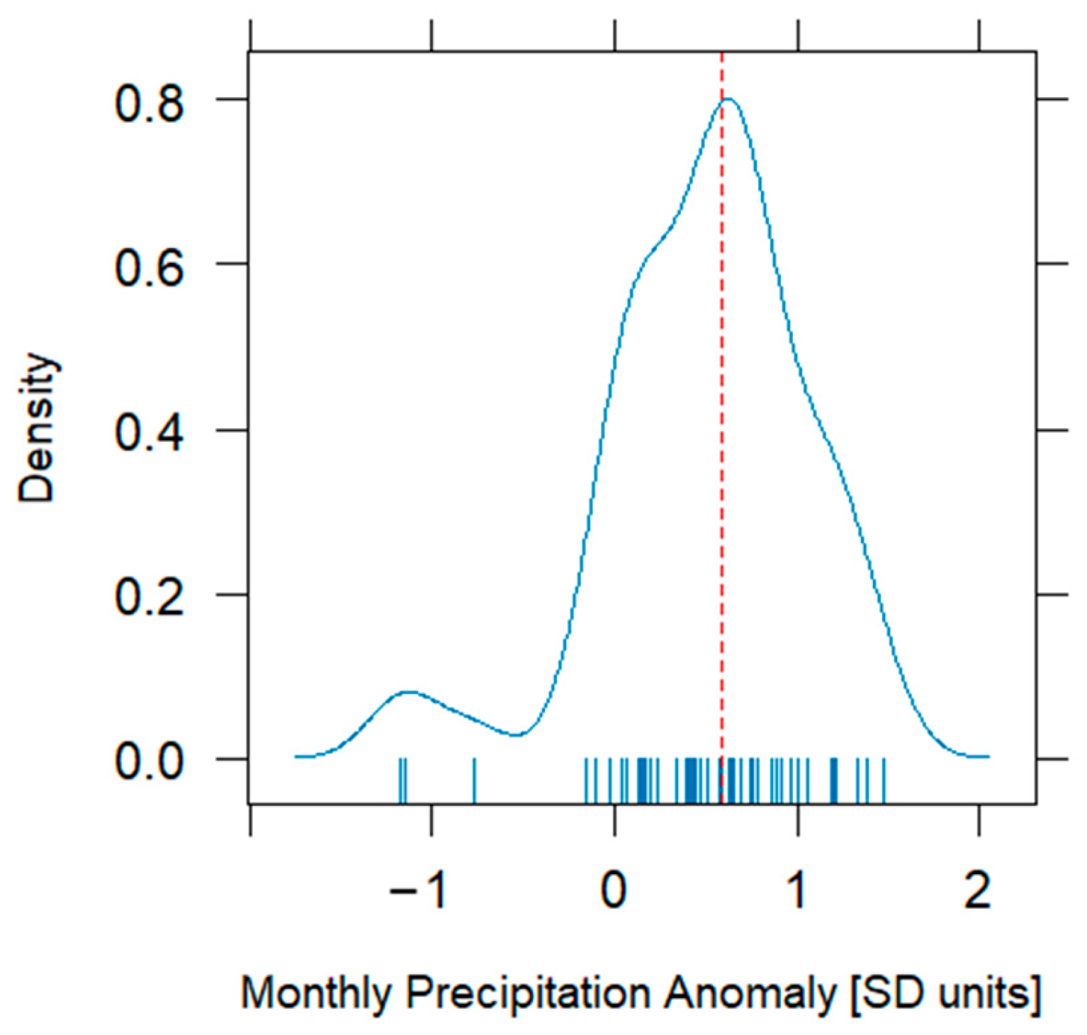
Therefore, we used a standardized precipitation anomaly threshold of 0.6 SD that represents the median value of the monthly anomaly distribution. The distribution in Figure 2 shows a longer left tail (negative anomalies) due to the driest months. The median allows a balance between the binary classes of the response variable, disregarding outliers’ effects. This threshold also allows for a distinction between wetter-than-normal and more average conditions across the climatic gradient associated with odds of landslide occurrence. For each landslide location, if the standardized rainfall anomaly grid-box was greater than 0.6, then the event was ranked as likely being driven by rainfall (1). Landslides accompanied by values of standardized rainfall less than 0.6 were ranked as non-likely driven by rainfall (0) (Equation (1)).
Y = { 1   i f   l a n d s l i d e   o c c u r r e n c e   d r i v e n   b y   r a i n f a l l 0   i f   l a n d s l i d e   o c c u r r e n c e   n o t   d r i v e n   b y   r a i n f a l l                        
(2)
Multicollinearity analysis. Multicollinearity among predictors was assessed to ensure model stability and avoid redundancy. This phenomenon occurs when independent variables are highly correlated, leading to inflated variance, numerical instability, and reduced predictive performance [40,41]. Although diagnostics in generalized linear models are ideally based on the information matrix, an initial screening was conducted using pairwise visual inspection.
(3)
Independence of categorical variables. The three categorical variables were evaluated for statistical independence using the Chi-square test [42]. We used this test to check for independence among groups of categorical variables because we suspected that data manipulation of lithological, land use and vegetation cover classes could influence the distribution of categorical variables. This test assesses whether observed frequencies differ significantly from expected frequencies under the null hypothesis of independence. Its application requires two categorical variables with at least two groups each, independent observations, and sufficiently large expected frequencies (≥1 in all cells and ≥5 in at least 80% of them). The hypotheses were defined as follows: H0: variables are independent; H1: variables are dependent; significance level of α = 0.05. The test compares observed and expected frequencies across contingency tables to determine whether associations between variables are statistically significant (Equation (2)).
χ 2 =     i = 1 R j = 1 C ( o i j e i j ) 2 e i j
where oij is the observed cell count in the ith row, R, and jth column, C, of the table. The term eij is the expected cell count in the ith row and jth column of the table if the null hypothesis is assumed to be true, i.e., the joint probabilities of both variables are equal to individual probabilities multiplied together (Equation (3)) [43].
e i j = r o w   i   t o t a l c o l   j   t o t a l t o t a l   o b s e r v a t i o n s
The calculated χ2 value is then used to obtain a p-value from the right-tailed χ2 distribution with degrees of freedom df = (R − 1)(C − 1). This value is the probability, under the null hypothesis, that the observed χ2 value could be obtained by random chance [40], and it must be equal to or larger than the chosen level of significance, α.
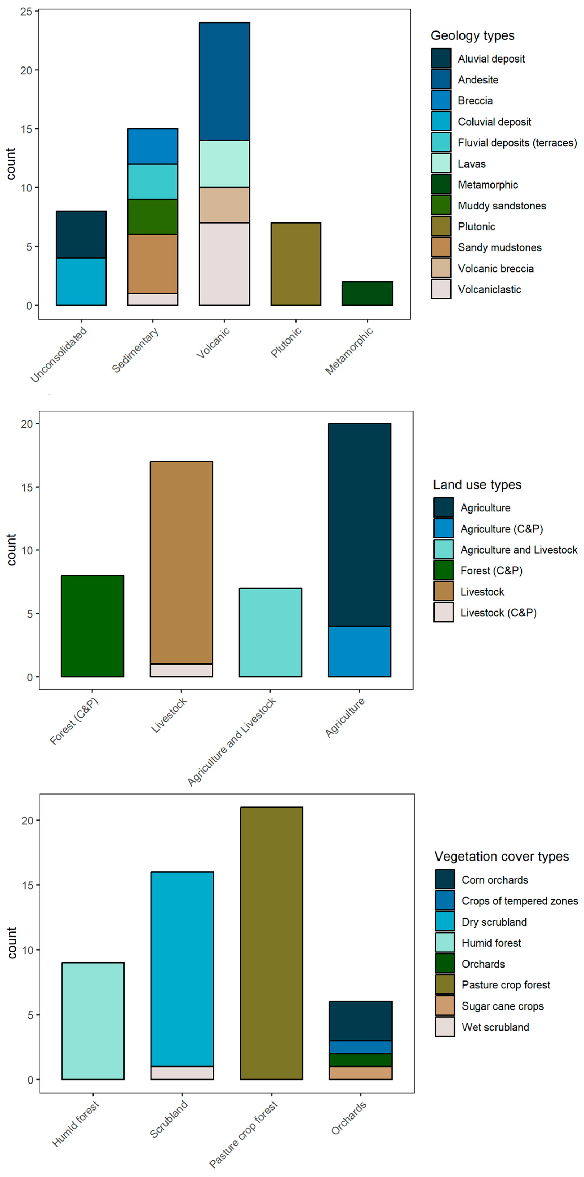
Adequate sample size is critical in logistic regression due to the use of maximum likelihood estimation, with recommended minimum sizes exceeding 100 observations [44]. Given the limited dataset, categorical variables were reclassified to improve robustness and reduce sparsity, observing reported trends in land use and agricultural activities on degraded Andean ecosystems [45]. The recategorization included the following: (1) merging dry and wet scrubland into a single “scrubland” class; (2) grouping temperate crops, corn orchards, and orchards into an “orchards” category; (3) removing poorly represented classes (páramo vegetation, shrub–herbaceous vegetation, and wasteland), reducing the dataset from 56 to 52 observations; and (4) consolidating livestock and agricultural subclasses into broader “livestock” and “agriculture” categories. These adjustments improved category balance for modeling purposes, as summarized in Table 2. Categorical variables (Figure 3) show that dominant vegetation covers include pasture-related areas, scrublands, and humid forests, while land use is mainly represented by livestock and agriculture. Livestock areas correspond primarily to pasture and natural grazing lands; forests represent protected or mixed forest–pasture systems; agriculture includes crops such as maize and sugarcane; and mixed-use areas reflect combined livestock–agriculture practices.

2.2.3. Exploratory Analysis

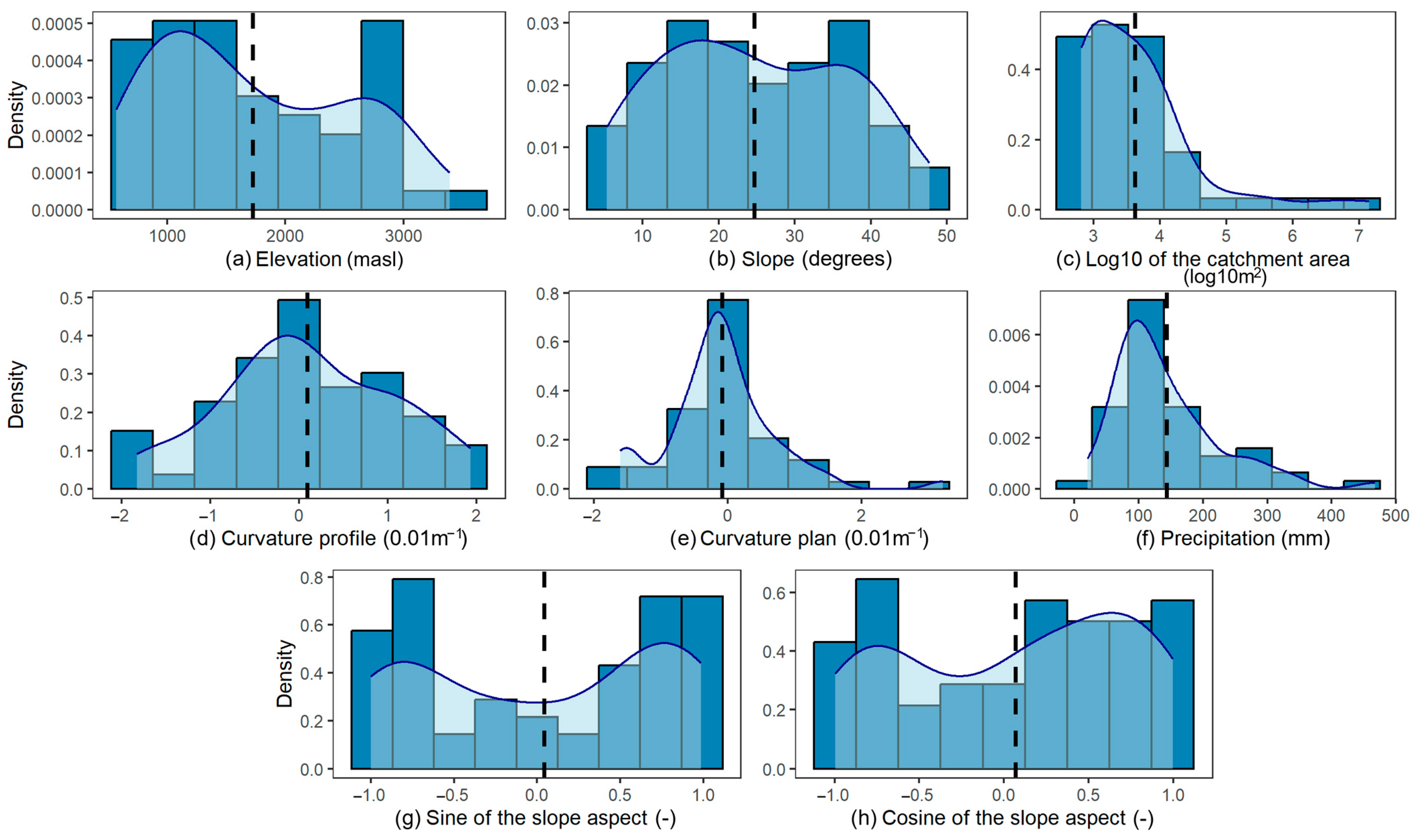
To characterize variable behavior, exploratory analysis was conducted using summary statistics and distribution plots. The summary statistics indicated no significant outliers within the landslide sample (Table 3). Histograms of continuous variables (Figure 4a–h) reveal heterogeneous scales and predominantly non-Gaussian distributions. Profile curvature exhibits a platykurtic distribution, while plan curvature is leptokurtic. Precipitation and the log10 of catchment area are positively skewed and approximately mesokurtic. Elevation, slope, and the sine and cosine of aspect display bimodal distributions, showing that landslides occur across contrasting topographic conditions (e.g., both low and high elevations and slopes). Given these characteristics, data normalization was applied to standardize variable scales.

2.3. Regression Models

The methodology adopts a classification framework to predict a qualitative response, specifically landslide occurrence [46]. Two statistical approaches—Generalized Linear Models (GLM) and Generalized Additive Models (GAM)—are employed in a stepwise manner to model the relationship between the binary response variable and multiple predictor variables representing landslide drivers. Model selection is performed based on the Akaike Information Criterion (AIC), and its ability to distinguish between the binary classes is evaluated using the Area Under the Receiver Operating Characteristic Curve (AUC–ROC), which assesses the ability of the models to discriminate between rainfall-driven landslide and non-rainfall driven landslide conditions.

2.3.1. Generalized Linear Model (GLM)

GLM extends classical linear models by allowing the response variable Y to follow different distributions (e.g., binomial, Poisson, gamma, normal) and by incorporating multiple predictors, including transformed variables. This framework enables modeling of both continuous and categorical responses. A GLM consists of three components: (1) Systematic component: predictors, coefficients, and constants. (2) Random component: the response variable and its probability distribution (from the exponential family). (3) Link function: a monotonic function that relates the expected value of the response to the linear predictor, transforming it to an unbounded scale. The general structure of a GLM is as Equation (4):
g ( μ i ) = X i β
where μ i = E ( Y i ) , g ( ) is the link function (e.g., logit in logistic regression), X i is the vector of predictors for observation i , and b e t a is the vector of coefficients. GLMs assume the independence of observations and allow flexible modeling of non-normal data, making them suitable for applications such as landslide occurrence, where the response is binary.
Logistic regression is widely used in GLM for modeling binary responses, characterized by a binomial distribution and a logit link function. Instead of modeling the response variable directly, it estimates the probability of landslide occurrence given a set of predictors. The logit transformation relates this probability to a linear predictor (Equation (5)):
logit ( p ) = l o g ( p 1 p )
where p = Pr ( Y = 1 | X ) is the conditional probability of landslide occurrence. The term p 1 p represents the odds. The multiple logistic regression model is expressed as Equation (6):
l o g ( p 1 p ) = β 0 + β 1 x 1 + β 2 x 2 + + β n x n

2.3.2. Generalized Additive Models (GAM)

Although GLMs are widely used in landslide susceptibility analysis, their linearity assumption may be unrealistic in complex environmental systems, limiting predictive performance [7,34]. Generalized Additive Models (GAMs) address this limitation by extending GLMs to incorporate non-linear relationships while retaining interpretability [47]. GAMs are semi-parametric models in which the linear predictor is replaced by a sum of smooth functions applied to each predictor. For binary responses, the logistic formulation in Equation (6) is extended as in Equation (7):
l o g ( p 1 p ) = β 0 + f 1 ( X 1 ) + f 2 ( X 2 ) + + f n ( X n )
where f j ( X j ) are smooth functions (e.g., splines), whose complexity is controlled by degrees of freedom. These functions allow flexible modeling of non-linear effects, improving discrimination and predictive capability. GAMs offer advantages such as increased flexibility and the ability to evaluate individual predictor effects while holding others constant. However, they are less interpretable than linear models and require explicit inclusion of interaction terms when needed.

2.3.3. Receiver Operating Characteristic (ROC) Curves

ROC curves evaluate classifier performance by plotting the true positive rate against the false positive rate across thresholds. The Area Under the Curve (AUC) provides a measure of overall model accuracy, with higher values indicating better discrimination. In this study, AUC–ROC was used to assess and compare the predictive performance of GLM and GAM in distinguishing between rainfall-driven and non-rainfall driven landslide occurrences. The GLM and GAM were fitted using the “glm ()” and “gam ()” functions from the open-source software R (R Core Team, Vienna, Austria, version 4.5.1) [48].

3. Results

3.1. Dataset Quality Control

The Chi-square test indicates that combinations involving the geology attribute yield chi-square test statistics exceeding the critical value (or p-values below α = 0.05), leading to rejection of the null hypothesis of independence. In contrast, vegetation cover and land use show no significant association (p-value > 0.05), suggesting independence (Appendix A).
Multicollinearity among continuous predictors was assessed using Pearson correlation coefficients, adopting a threshold of |r| > 0.7 as indicative of high collinearity [49] (Figure S1). None of the variables exceeded this threshold, indicating that all predictors could be retained without significant multicollinearity concerns. However, moderate correlations were observed between precipitation and elevation and between plan and profile curvature, which should be considered when interpreting model results.

3.2. Logistic Modeling Approach

Several model structures were fitted, starting with a simple null model and moving to more complex structures. We chose a building block modeling strategy that started from the null model to test the rainfall effect by adding first single topographic effects on the one hand, then testing the grouped effects of land use and vegetation on the other hand to obtain a full linear model. Variance Inflation Factors (VIF) in Figure S2 for the full linear model show that all predictors are below a VIF threshold of 5, meaning a low correlation among them. Then, polynomial quadratic and cubic terms were added progressively to topographic variables, one per iteration until no further decrease in the AIC was achieved. A critical concern is that the independence assumption underlying GLM and GAM holds for the small sample of landslide occurrences, as nearby landslides are likely to share similar environmental conditions. We assessed this through a residual plot (Figure S3) of the full linear model including all continuous and categorical predictors. The plot shows spreading of residuals and no obvious patterns.
We implemented a manual stepwise AIC-based model selection rather than an algorithm-based one. We prefer this choice as it provides control over the model fitting and takes advantage of the transparency and theoretical plausibility of identified predictors. The GLM space for the full linear model parameter learning might appear over-specified and the risk of overfitting is plausible when exploring the pool of causal predictors. However, the proposed GLM is an explanatory model intended to infer cause–effect relationships between climatic forcing (monthly rainfall totals), a set of environmental factors and rainfall-related landslides occurrences. As such, overfitting is indeed plausible as it arises from methodological assumptions. This, however, does not have damming effects for the modeling framework since the goal is to test all causal hypotheses on theoretical constructs.
In the presence of overfitting, one might consider a simplification of the fitted GLM via penalized regression models, which also addresses limitations of stepwise AIC selection methods. Alternative penalized regression methods such as Ridge and Lasso regression are instrumental in constraining coefficients towards zero. Nevertheless, they are not ideally suited for our modeling purpose. For example, Ridge regression shrinks predictors towards zero, but keeping them makes model interpretation cumbersome. Lasso regression, on the other hand, shrinks parameters to zero but drops others. In our explanatory modelling setting, one might need to choose to retain a causal covariate because of strong theoretical or empirical justifications.
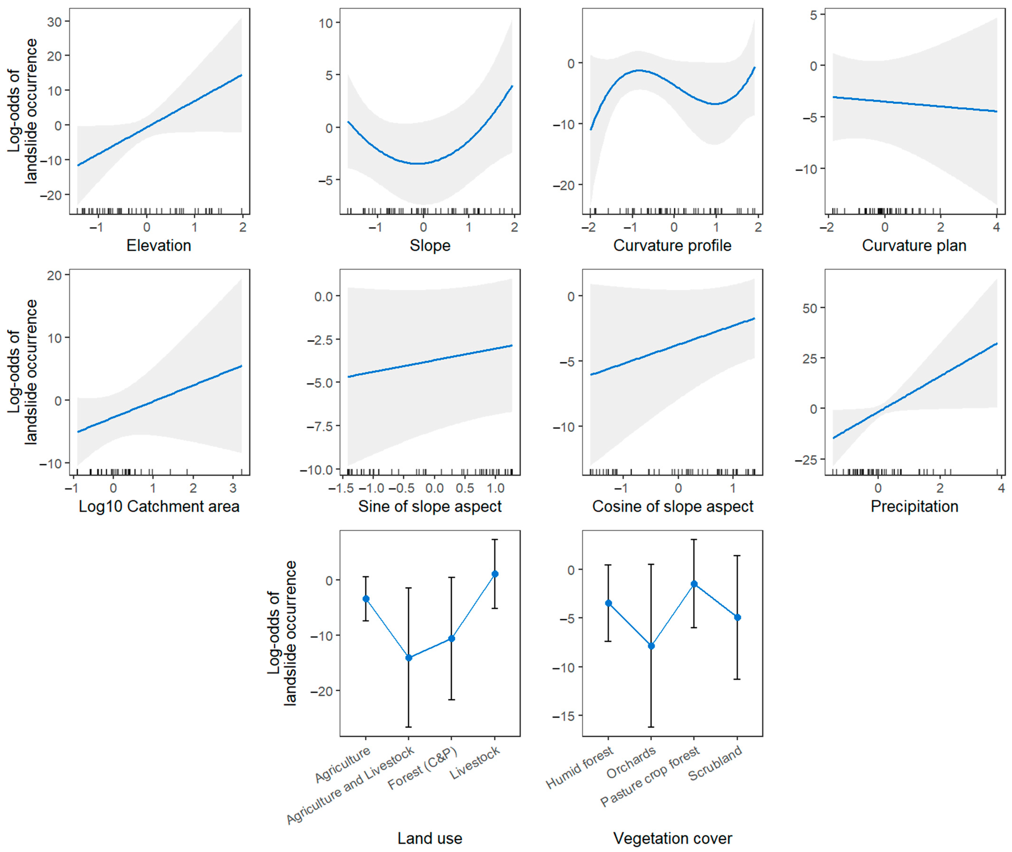
The selected logistic regression model included land use, vegetation cover, elevation, linear plan curvature, log10 catchment area, sine and cosine of slope aspect, precipitation, a second-degree polynomial for slope, and a third-degree polynomial for profile curvature (Figure 5). This model structure retained interpretable environmental predictors while allowing nonlinear responses for slope and profile curvature, two variables whose effects may not be adequately represented by simple linear terms. The model showed an adequate overall fit, with the null deviance decreasing from 72.09 on 51 degrees of freedom to a residual deviance of 26.24 on 34 degrees of freedom. The resulting AIC was 62.24, indicating improved fit relative to the intercept-only model. The model converged after nine Fisher scoring iterations, and the deviance residuals were approximately centered around zero, suggesting that the model adequately captures the underlying relationship in the data.
Because the continuous predictors were normalized prior to model fitting, their coefficients represent changes in the log-odds of landslide occurrence per one standardized unit increase in the predictor. In contrast, coefficients for categorical predictors represent differences in log-odds relative to their reference categories. Therefore, land-use and vegetation-cover effects should be interpreted as relative effects, rather than absolute differences among all classes.
Model coefficients (Table 4) identify precipitation, the second-order slope polynomial term, and agriculture–livestock land use as statistically significant predictors at the 5% level. Elevation showed a positive but marginally significant effect at the 10% level, while forest conservation and protection land use showed a marginal negative association at the 10% level.
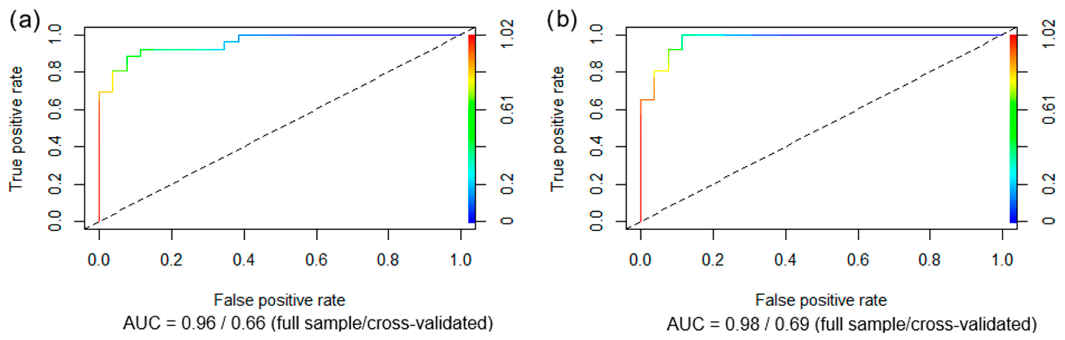
Overall, the best GLM achieved a full-sample AUC–ROC of 0.957, dropping to a cross-validated AUC-ROC of 0.66. The former value reflects model’s ability to separate the observed landslide occurrence classes; however, since it was calculated using fitted values from the full dataset, it should be interpreted as apparent model performance. Model predictive performance was assessed by implementing stratified train/test validation on 200 samples and computing metrics from the holdout set, yielding a mean AUC of 0.66. This shows that the best GLM performs modestly in a predictive setting, this being a key limitation. The distinction is important because the dataset is relatively small and includes several categorical predictors with limited observations per class. Thus, the cross-validated predictive performance should be regarded as the performance metric to avoid overoptimistic predictive accuracy drawn from the full-sample explanatory model.

3.3. Generalized Additive Models

Using the same dataset, GAM candidates were fitted assuming a binomial error distribution with a logit link. The modeling strategy involved introducing low-rank smoothers on the elevation, slope and curvature profiles as they showed nonlinear behaviors on the partial-effect plot while exploring some model structures in the GLM fitting. The focus was on balancing model fit with complexity. Among the tested models, the best GAM achieved an AIC of 50.61 and a high discriminatory performance, with full-sample AUC of 0.976 (Figure 6b) dropping to a cross-validated AUC-ROC of 0.69, indicating slightly better performance than the GLM (Figure 6a).
Model comparison using sequential analysis of deviance (Table 5) indicated that Model 2 provided a significant improvement over Model 1, with a reduction in residual deviance of 19.014 and a chi-square p-value of 0.0001206. In contrast, Model 3 did not significantly improve the model fit relative to Model 2 (p = 0.5998). Therefore, Model 2 was retained as the preferred GAM. This model included smooth terms for elevation and profile curvature, while retaining slope as a linear predictor. The smooth terms had low effective degrees of freedom, with elevation showing modest nonlinear behavior (edf = 1.911) and profile curvature behaving approximately linearly (edf = 0.947). Thus, the selected GAM improved predictive performance while maintaining a relatively simple and geomorphologically interpretable structure.
Additionally, the parametric coefficients indicate that precipitation was the only predictor significant at the 5% level in the selected GAM (estimate = 15.84, p = 0.03; Table 6). This positive coefficient suggests that higher precipitation is associated with increased log-odds of landslide occurrence. The cosine of slope aspect also showed a positive effect, but only marginally (p = 0.10), while the sine of slope aspect was similarly positive but not statistically significant at the 5% level (p = 0.12). In contrast, the agriculture–livestock land-use class had a negative coefficient, but this effect was not statistically significant (p = 0.46), so it does not show strong evidence of reduced rainfall-related landslide occurrence. Among the smooth terms, elevation showed modest nonlinear behavior, with an effective degree of freedom value close to 2 (edf = 1.91, p = 0.095), while profile curvature was close to linear or weakly nonlinear (edf = 0.95, p = 0.052; Table 6).

4. Discussion

4.1. Dataset

The Chi-square test used to shed light on the effect of the data manipulation step reported that lithological classes had strong associations with land use and vegetation classes. The high level of manipulation, e.g., class reductions from 59 to 12 for lithology versus 10 to 6 for land uses and 12 to 8 for vegetation cover, could affect the independence and statistical relevance of this categorical variable for shallow landslides. Therefore, the geological attribute variables were excluded from subsequent analyses.
The final dataset of environmental predictors consisted of climatological (monthly precipitation anomalies) and topographic (elevation, slope, curvature plan and profile, log 10 catchment area, sine and cosine of the slope) continuous variables. Additionally, land use (agriculture, agriculture and livestock, forest crops and pastures, livestock) and vegetation cover (humid forest, orchards, pasture crop and forest, scrubland) were used as categorical variables.

4.2. Logistic Modeling Approach

Parameter estimates from the logistic regression model show that a one-standard-deviation increase in precipitation, equivalent to 84.13 mm in the original scale, substantially increases the log-odds of landslide occurrence, by a factor of 8.84. Elevation also showed a positive effect, suggesting that landslide occurrence tends to increase along environmental gradients associated with higher-elevation terrain, although this relationship was only marginally significant. In contrast, agriculture–livestock land use showed a strong negative association relative to the reference land-use class. This finding contrasts with previous studies [50] and suggests the need for further investigation, as the limited sample size, map resolution, land-use classification, irrigation practices, and local land-cover management can influence the observed response, but they are not fully represented in the available thematic maps.
Partial-effect plots illustrate these relationships (Figure 5). Precipitation shows the clearest positive effect, with landslide log-odds increasing sharply across the standardized precipitation gradient. Elevation also shows a positive trend, although uncertainty increases across the range of observed values. The slope effect is nonlinear, consistent with the significant second-order polynomial term, indicating that slope does not influence landslide occurrence through a simple linear relationship. Profile curvature and log10 catchment area show curved or positive tendencies, but their coefficients are not statistically significant. Vegetation-cover classes and slope-aspect terms also show no significant effects at the 5% level, although the cosine of slope aspect remains positively associated with landslide occurrence.

4.3. Generalized Additive Models

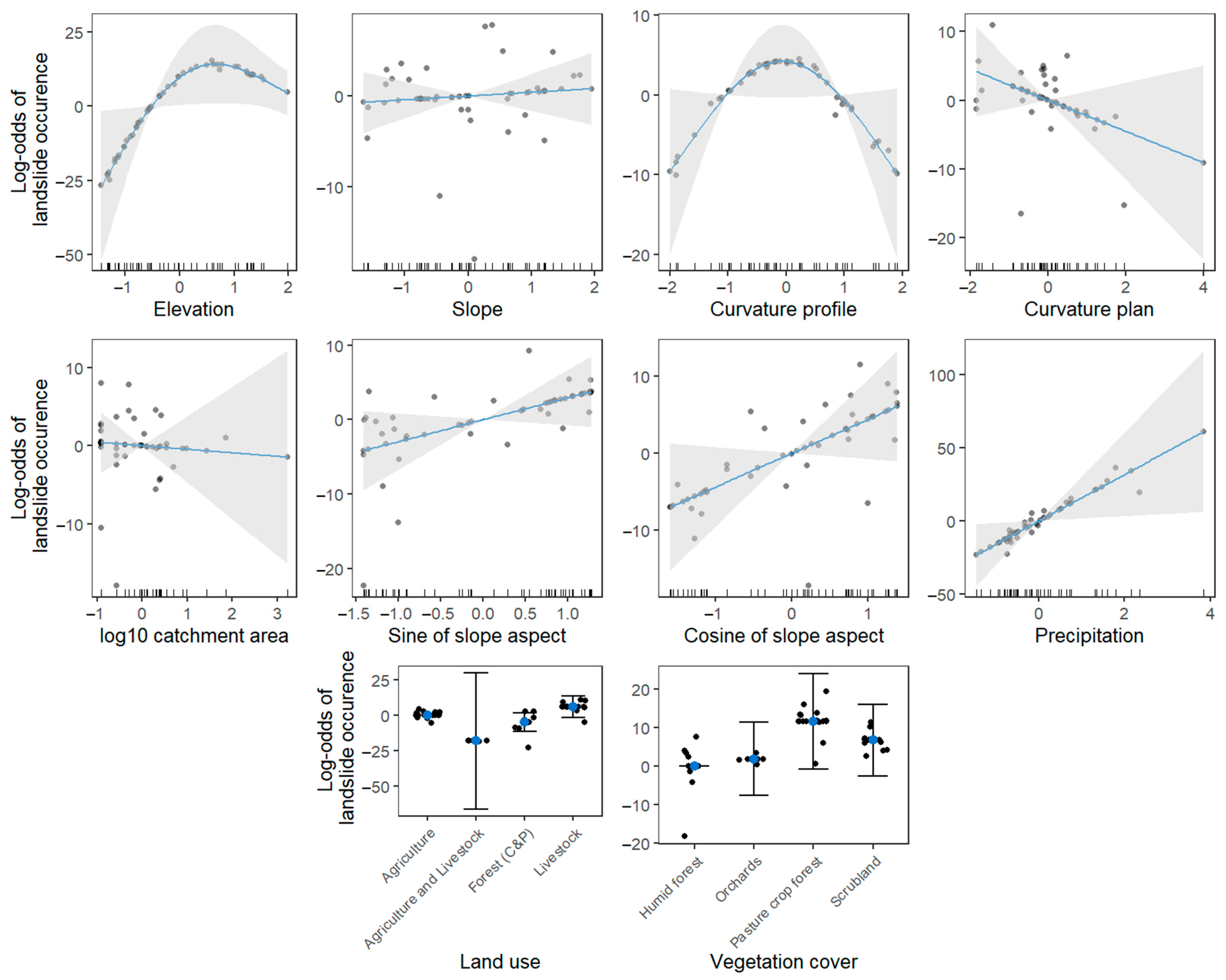
Overall, the GAM results suggest that precipitation and selected topographic variables contribute to rainfall-related landslide occurrence, while the smooth terms capture limited but geomorphologically meaningful nonlinearities. The partial-effect plots further illustrate these relationships (Figure 7). Elevation shows a curved response, with landslide log-odds increasing at the intermediate elevation range, around the sample mean to one-positive standard deviation (~1727–2532 masl). Profile curvature also displays a nonlinear pattern with higher predicted log-odds near mean intermediate curvature values (−1 to 1), showing that moderate hilly areas, both upwardly convex and concave, increase the log-odds of landslide occurrence. In contrast, slope shows a relatively weak or nearly flat partial effect after accounting for the other predictors, although it was retained because of its mechanistic importance in landslide processes. The precipitation panel shows a strong positive trend, consistent with the significant positive coefficient reported in Table 6. The aspect terms also show positive tendencies, particularly for cosine of slope aspect, suggesting that north-east/-west oriented slopes increase the log-odds of landslide occurrence but with wider uncertainty. Together, the coefficient table and partial-effect plots indicate that the selected GAM captures both the positive effects of precipitation and moderate nonlinear responses associated with elevation and profile curvature.
We noticed that land-use effects were not consistent between GLM and GAM. This is explained by the difference in fitting assumptions among models. While GLM makes uses of quadratic and cubic terms to model topographic effects, the GAM uses prescribed low-order splines to capture such effects in the same model space. The fitting of specified GAM smooth functions for topographic effects constrains or modifies the model space for the learning and fitting of land use and vegetation parameters, leading to slight differences in parameter values and statistical significance between GLM and GAM.

4.4. On the Application of the Assessment Framework in Other Contexts

While GLM and GAM are standard techniques for susceptibility modeling, such applications often rely on algorithm-based model selection, e.g., forward and backward elimination. Instead, we use a building block modelling strategy which, starting with the null model, tests rainfall effects by progressively adding first topographic variables then lumped effects of land use and vegetation cover. In the GLM setting, quadratic and cubic terms are added gradually to topographic predictors. In the GAM setting, polynomial terms are replaced by low-order splines. Thus, the modelling strategy is designed to allow a natural representation of expected topographic relationships based on heuristic knowledge. In our study case, the results show that deviations from mean values of monthly precipitation raise the odds of landslides occurrence under the assumed normal and wetter-than-normal conditions, but they also show that rainfall should be interpreted jointly with topographic and land-cover controls. Landslides were more likely to occur under wetter conditions at intermediate elevations and on northwestern facing slopes where ground moisture gradients condition slope stability, which is relevant for the target region but also for other mountainous regions where knowledge of such interaction is still incipient.
Tropical and humid mountainous regions share challenges in landslide susceptibility analysis, such as short and low-quality landslide records and geo-environmental information where landslide triggers are thought to originate mostly from rainfall. In this paper, we showed that despite those limitations, stepwise GLM and GAM are useful approaches to classify rainfall-driven and non-rainfall driven landslides within confounding environmental factors. The intelligibility and transparency of a regression-type method plus a minimal consistence criterion to validate the identified landslide drivers should make this approach an adequate framework to support landslide characterization in other tropical mountainous regions.

5. Conclusions

Landslides are complex geohazards driven by interactions between predisposing and triggering factors, yet their dynamics in data-scarce environments such the northern Ecuadorian Andes remain insufficiently understood. Predisposing factors—such as topography, geology, and long-term human impacts on land cover—control slope susceptibility, while triggers including intense rainfall, earthquakes or anthropogenic disturbances initiate failure events. Despite some advances in monitoring and plot-scale physically based investigations in northern Ecuador, the vast array of triggering mechanisms and their interactions with confounding environmental factors are still not fully understood, often oversimplifying the role of rainfall as the sole driver.
To address this gap, a curated dataset of landslides for the Imbabura Province was developed, integrating terrain attributes (elevation, slope, curvature, catchment area, and aspect), topological variables (vegetation cover and land use), and precipitation. These variables were used to model landslide occurrence through both a Generalized Linear Model (GLM) and a Generalized Additive Model (GAM), incorporating triggering conditions to better capture cause–effect relationships.
Despite data limitations—such as short landslide records and the availability of high-resolution cartographic information—both models were demonstrated to be instrumental for explanatory modeling purposes but to have limitations in a predictive setting, with the GAM providing modest improvement. The selected GLM achieved an AUC of 0.66, while the selected GAM achieved a higher AUC of 0.69. The improvement seen in the GAM reflects the value of allowing nonlinear relationships, particularly for elevation and profile curvature. Although we did not expect the proposed explanatory model to be optimal in terms of predictive power, it shows some limited to modest accuracy. If one considers the relatively small sample size, e.g., <5 events per predictor variable, which makes the model prone to overfitting, as well as the use of the full dataset for model evaluation, the apparent predictive performances, AUC values, are high. The contrast between the explanatory and predictive model performances represents the sacrifice in reducing the bias of the overoptimistic explanatory model intended for causal inference in return for a combined reduction in bias and variance in its cross-validated version.
Precipitation deviations from mean monthly values, larger within December–April but also important during less wet periods in the year, raise the odds of landslide occurrence. In the GLM, precipitation had a strong positive effect on landslide occurrence, and in the selected GAM it was the only parametric predictor significant at the 5% level. The results therefore unveil its importance as a trigger of landslide occurrences under the assumed normal and wetter-than-normal conditions, but they also show that rainfall should not be interpreted in isolation from topographic and land-cover controls.
Topographic predictors further contributed to rainfall-related landslide occurrence. Elevation showed a positive marginal effect in the GLM and a modest nonlinear response in the GAM, suggesting that landslide occurrence varies along environmental gradients associated with temperature, humidity, vegetation distribution, and ground saturation. Profile curvature also showed weak nonlinear behavior in the selected GAM, implying high odds of landslide occurrence across the base of slopes to the crests of hills; slope was retained as a mechanistically important predictor even though its statistical effect was not significant in the final GAM. The cosine of slope aspect showed a positive but marginal association, suggesting that slope orientation may influence local moisture conditions, although this effect should be cautiously regarded because of its uncertainty.
Land-use effects were less consistent. Agriculture–livestock land use showed a strong negative association in the GLM, but this effect was not significant in the selected GAM. This discrepancy suggests that land-use effects are sensitive to model structure, sample size, and the spatial resolution of the available thematic maps.
Overall, this study demonstrates that combining curated landslide records with GLM and GAM approaches can provide a useful baseline for rainfall-related landslide occurrence assessments in data-scarce Andean regions. Future work should prioritize improving landslide inventories, incorporating independent validation datasets, refining land-use and vegetation-cover information at higher spatial resolution, and including additional process-based variables such as high-resolution lithology, accurate road proximity distances, soil properties such as depth, texture and hydraulic conductivity, antecedent rainfall, and rainfall intensity–duration thresholds. These improvements would strengthen the interpretation of cause–effect relationships and support more robust rainfall-related landslide occurrence modeling in northern Ecuador.

Supplementary Materials

The following supporting information can be downloaded at https://www.mdpi.com/article/10.3390/geohazards7040108/s1, Figure S1: Collinearity test among attributes. The colored dots represent landslides categorized by type of rock (red: metamorphic, blue: plutonic, green: sedimentary, orange: unconsolidated, yellow: volcanic), Figure S2: Variance inflation factors of the full GLM, Figure S3: Plot of residuals of the full GLM.

Author Contributions

Conceptualization, L.E.P. and A.R.; methodology, L.E.P. and A.R.; formal analysis, A.R.; investigation, A.R. and L.E.P.; data curation, A.R.; writing—original draft preparation, A.R.; writing—review and editing, A.R. and L.E.P.; funding acquisition, L.E.P. All authors have read and agreed to the published version of the manuscript.

Funding

This research was funded by the Ecuadorian National Under-Secretary of Science, Technology and Innovation, grant number 01001113 IDEARIUM-PIC-24-CONEC-YACHAY-001 ‘Sistema para la identificación de anomalías meteorológicas en el Ecuador’.

Data Availability Statement

The original contributions presented in this study are included in the article/Supplementary Material. Further inquiries can be directed to the corresponding author.

Acknowledgments

A.R. and L.E.P. thank the ‘Instituto Nacional de Meteorología e Hidrología’ and ‘Ministerio de Agricultura y Ganadería de Ecuador’ for making hydrometeorological and thematic geographical information publicly available. During the preparation of this manuscript, the authors used ChatGPT (OpenAI GPT5.2) for the purposes of reviewing and improving the English language. The authors have reviewed and edited the output and take full responsibility for the content of this publication.

Conflicts of Interest

The authors declare no conflicts of interest.

Appendix A

Table A1. Chi-square test statistics for independence between the three categorical attributes, with both p-value and critical value approaches, for a significance level 0.05.
Attributes\Valuesχ2dfCritical ValueRejection Zonep-ValueReject
Geology vs. Land use118.197798.48[98.48, ∞)0.00178Yes
Geology vs. Veg cover137.5888110.89[110.89, ∞)0.00057Yes
Veg cover vs. Land use71.175674.46[74.46, ∞)0.08322No
The associated p-values of the computed χ2 show that the probability, under the null hypothesis of independence, to obtain the observed χ2 value could increase by random chance.

References

  1. Soto, J.; Palenzuela, J.A.; Galve, J.P.; Luque, J.A.; Azañón, J.M.; Tamay, J.; Irigaray, C. Estimation of empirical rainfall thresholds for landslide triggering using partial duration series and their relation with climatic cycles. An application in southern Ecuador. Bull. Eng. Geol. Environ. 2019, 78, 1971–1987. [Google Scholar] [CrossRef] [Scilit]
  2. López Cevallos, F.D. Utilización de un SIG para Establecer Zonas de Afectación por Amenazas Naturales: Sismos, Erupciones Volcánicas y Deslizamientos: Posibles Consecuencias en la Salud de la Población en la Parroquia Tababela. Undergraduate Thesis, Universidad San Francisco de Quito, Quito, Ecuador, 2004. Available online: https://repositorio.usfq.edu.ec/bitstream/23000/478/1/75856.pdf (accessed on 15 March 2021).
  3. Buitrón Vinueza, S.M. Metodología y Modelo para Movimientos en Masa Utilizando Técnicas de SIG y Teledetección. Undergraduate Thesis, Universidad San Francisco de Quito, Quito, Ecuador, 2014. Available online: http://repositorio.usfq.edu.ec/handle/23000/3849 (accessed on 15 March 2021).
  4. Younes Cárdenas, N.; Erazo Mera, E. Landslide susceptibility analysis using remote sensing and GIS in the western Ecuadorian Andes. Nat. Hazards 2016, 81, 1829–1859. [Google Scholar] [CrossRef] [Scilit]
  5. Domínguez, R.Z. El deslizamiento de La Josefina “Tragedia Nacional”. Galileo 2014, 1, 87–98. [Google Scholar]
  6. Hen-Jones, R.; Zapata, C.; Jiménez, E.; Holcombe, E.A.; Vardanega, P.J. Community-scale slope stability assessment of urbanisation scenarios in North Quito, Ecuador. Landslides 2026, 23, 55–71. [Google Scholar] [CrossRef] [Scilit] [PubMed]
  7. Brenning, A.; Schwinn, M.; Ruiz-Páez, A.P.; Muenchow, J. Landslide susceptibility near highways is increased by 1 order of magnitude in the Andes of southern Ecuador, Loja province. Nat. Hazards Earth Syst. Sci. 2015, 15, 45–57. [Google Scholar] [CrossRef] [Scilit]
  8. Puente-Sotomayor, F.; Mustafa, A.; Teller, J. Landslide Susceptibility Mapping of Urban Areas: Logistic Regression and Sensitivity Analysis applied to Quito, Ecuador. Geoenviron. Disasters 2021, 8, 19. [Google Scholar] [CrossRef] [Scilit]
  9. Bravo-López, E.; Fernández Del Castillo, T.; Sellers, C.; Delgado-García, J. Analysis of Conditioning Factors in Cuenca, Ecuador, for Landslide Susceptibility Maps Generation Employing Machine Learning Methods. Land 2023, 12, 1135. [Google Scholar] [CrossRef] [Scilit]
  10. Wieczorek, G.F. Chapter 4: Landslide Triggering Mechanisms. In Landslides: Investigation and Mitigation; Turner, A.K., Schuster, R.L., Eds.; Transportation Research Board Special Report; The National Academies Press: Washington, DC, USA, 1996; pp. 76–90. Available online: https://www.scirp.org/reference/referencespapers?referenceid=1438034 (accessed on 1 December 2020).
  11. Borgatti, L.; Vittuari, L.; Zanutta, A. Geomatic methods for punctual and areal control of surface changes due to landslide phenomena. In Landslides: Causes, Types and Effects; Nova Science Publishers: New York, NY, USA, 2010; p. 417. [Google Scholar]
  12. Crosta, G.B.; Frattini, P. Distributed modelling of shallow landslides triggered by intense rainfall. Nat. Hazards Earth Syst. Sci. 2003, 3, 81–93. [Google Scholar] [CrossRef] [Scilit]
  13. Ochoa, A.; Pineda, L.; Crespo, P.; Willems, P. Evaluation of TRMM 3B42 precipitation estimates and WRF retrospective precipitation simulation over the Pacific-Andean region of Ecuador and Peru. Hydrol. Earth Syst. Sci. 2014, 18, 3179–3193. [Google Scholar] [CrossRef] [Scilit]
  14. Springman, S.; Kienzler, P.; Casini, F.; Askarinejad, A. Landslide triggering experiment in a steep forested slope in Switzerland. In Proceedings of the 17th International Conference on Soil Mechanics and Geotechnical Engineering: The Academia and Practice of Geotechnical Engineering, Alexandria, Egypt, 2 October 2009; IOS Press: Amsterdam, The Netherlands, 2009; pp. 1698–1701. [Google Scholar] [CrossRef] [Scilit]
  15. Soto, J.; Galve, J.P.; Palenzuela, J.A.; Azañón, J.M.; Tamay, J.; Irigaray, C. A multi-method approach for the characterization of landslides in an intramontane basin in the Andes (Loja, Ecuador). Landslides 2017, 14, 1929–1947. [Google Scholar] [CrossRef] [Scilit]
  16. DesInventar (LatinAmerican Network of Social Studies on Disaster Prevention, LA RED). DesInventar. Available online: http://www.desinventar.lk:8081/DesInventar/help/welcometo.jsp (accessed on 1 June 2020).
  17. Farinango, C.; Geovanny, E. Estudio Geológico del Paleógeno en la Cordillera Occidental Septentrional del Ecuador, Provincias de Carchi e Imbabura. Undergraduate Thesis, Escuela Politécnica Nacional, Quito, Ecuador, 2014. Available online: https://bibdigital.epn.edu.ec/handle/15000/8867 (accessed on 15 March 2021).
  18. Ruiz, G.M.H. Exhumation of the Northern Sub-Andean Zone of Ecuador and Its Source Regions: A Combined Thermochronological and Heavy Mineral Approach. Doctoral Thesis, ETH Zurich, Zurich, Switzerland, 2002. Available online: https://www.research-collection.ethz.ch/bitstreams/425f183b-b4fd-4e74-ad7d-86864e41f6c1/download (accessed on 15 March 2021).
  19. Toro Álava, J.; Jaillard, E. Provenance of the Upper Cretaceous to upper Eocene clastic sediments of the Western Cordillera of Ecuador: Geodynamic implications. Tectonophysics 2005, 399, 279–292. [Google Scholar] [CrossRef] [Scilit]
  20. Vallejo Cruz, C. Evolution of the Western Cordillera in the Andes of Ecuador (Late Cretaceous-Paleogene). Doctoral Thesis, ETH Zurich, Zurich, Switzerland, 2007. Available online: http://e-collection.library.ethz.ch/view/eth:29746 (accessed on 15 March 2021).
  21. Baby, P.; Rivadeneira, M.; Barragán, R.; Christophoul, F. Thick-Skinned Tectonics in the Oriente Foreland Basin of Ecuador; Geological Society, London, Special Publications; The Geological Society of London: Bath, UK, 2013; Volume 377, pp. 59–76. [Google Scholar] [CrossRef] [Scilit]
  22. Instituto de Investigación Geológico Energético. Geologic Maps (Otavalo, Ibarra, Pacto); Scale 1 100.000; INIGEMM: Quito, Ecuador; Britanic Mission: Keyworth, UK; IGM: Quito, Ecuador, 1979.
  23. Eidt, R.C. The climatology of South America. In Biogeography and Ecology in South America, 1st ed.; Fittkau, E.J., Illies, J., Klinge, H., Schwabe, G.H., Sioli, H., Eds.; Springer: Berlin/Heidelberg, Germany, 1969; Volume 18, pp. 54–81. [Google Scholar] [CrossRef] [Scilit]
  24. Emck, P. A Climatology of South Ecuador with Special Focus on the Major Andean Ridge as Atlantic-Pacific Climate Divide. Doctoral Thesis, Erlangen-Nürnberg University, Erlangen, Germany, 2007. Available online: https://open.fau.de/handle/openfau/477 (accessed on 15 March 2021).
  25. Bendix, J.; Lauer, W. Die Niederschlagsjahreszeiten in Ecuador und ihre klimadynamische Interpretation (Rainy Seasons in Ecuador and Their Climate-Dynamic Interpretation). Erdkunde 1992, 46, 118–134. [Google Scholar] [CrossRef] [Scilit]
  26. Morán-Tejeda, E.; Bazo, J.; López-Moreno, J.I.; Aguilar, E.; Azorín-Molina, C.; Sanchez-Lorenzo, A.; Martínez, R.; Nieto, J.J.; Mejía, R.; Martín-Hernández, N.; et al. Climate trends and variability in Ecuador (1966–2011). Int. J. Climatol. 2016, 36, 3839–3855. [Google Scholar] [CrossRef] [Scilit]
  27. Villacís, M.; Vimeux, F.; Denis, J. Analysis of the climate controls on the isotopic composition of precipitation (δ18O) at Nuevo Rocafuerte, 74.5°W, 0.9°S, 250 m, Ecuador. C. R. Géosci. 2008, 340, 1–9. [Google Scholar] [CrossRef] [Scilit]
  28. Gordillo, J.; Pineda, L.E. Unravelling runoff processes in Andean basins in northern Ecuador through hydrological signatures. Hydrol. Process. 2021, 35, e14354. [Google Scholar] [CrossRef] [Scilit]
  29. Brönnimann, C.S. Effect of Groundwater on Landslide Triggering. Doctoral Thesis, École Polytechnique Fédérale De Lausanne, Lausanne, Switzerland, 2011. [Google Scholar] [CrossRef] [Scilit]
  30. Werner, E.D.; Friedman, H.P. Landslides: Causes, Types and Effects; Nova Science Publishers: New York, NY, USA, 2010. [Google Scholar]
  31. Urgilez Vinueza, A.; Robles, J.; Bakker, M.; Guzman, P.; Bogaard, T. Characterization and Hydrological Analysis of the Guarumales Deep-Seated Landslide in the Tropical Ecuadorian Andes. Geosciences 2020, 10, 267. [Google Scholar] [CrossRef] [Scilit]
  32. Gad Provincial de Imbabura. Plan de Desarrollo de Ordenamiento Territorial de la Provincia de Imbabura, 2015–2035. 2018. Available online: https://www.imbabura.gob.ec/phocadownloadpap/K-Planes-programas/PDOT/PDOT%20IMBABURA%202015-2035.pdf (accessed on 1 June 2020).
  33. Zerathe, S.; Lacroix, P.; Jongmans, D.; Marino, J.; Taipe, E.; Wathelet, M.; Pari, W.; Smoll, L.F.; Norabuena, E.; Guillier, B.; et al. Morphology, structure and kinematics of a rainfall controlled slow-moving Andean landslide, Peru. Earth Surf. Process. Landf. 2016, 41, 1477–1493. [Google Scholar] [CrossRef] [Scilit]
  34. Goetz, J.N.; Guthrie, R.H.; Brenning, A. Integrating physical and empirical landslide susceptibility models using generalized additive models. Geomorphology 2011, 129, 376–386. [Google Scholar] [CrossRef] [Scilit]
  35. Brenning, A. Spatial prediction models for landslide hazards: Review, comparison and evaluation. Nat. Hazards Earth Syst. Sci. 2005, 5, 853–862. [Google Scholar] [CrossRef] [Scilit]
  36. Pourghasemi, H.R.; Rossi, M. Landslide susceptibility modeling in a landslide prone area in Mazandarn Province, north of Iran: A comparison between GLM, GAM, MARS, and M-AHP methods. Theor. Appl. Climatol. 2017, 130, 609–633. [Google Scholar] [CrossRef] [Scilit]
  37. JAXA. ALOS Global Digital Surface Model “ALOS World 3D—30m (AW3D30)”. 2020. Available online: https://www.eorc.jaxa.jp/ALOS/en/index_e.htm (accessed on 1 September 2020).
  38. International Research Institute for Climate and Society from Columbia University. Climate Data Library. Available online: https://iridl.ldeo.columbia.edu/ (accessed on 1 September 2020).
  39. Ministerio de Agricultura y Ganadería, Sistema Nacional de Información. Archivos de Información Geográfica; Ministerio de Agricultura y Ganadería: Quito, Ecuador, 2014. Available online: http://www.sigtierras.gob.ec/geoportal/ (accessed on 1 September 2020).
  40. Kuhn, M.; Johnson, K. Applied Predictive Modeling; Springer: Berlin/Heidelberg, Germany, 2013. [Google Scholar] [CrossRef] [Scilit]
  41. Chen, W.; Pourghasemi, H.R.; Panahi, M.; Kornejady, A.; Wang, J.; Xie, X.; Cao, S. Spatial prediction of landslide susceptibility using an adaptive neuro-fuzzy inference system combined with frequency ratio, generalized additive model, and support vector machine techniques. Geomorphology 2017, 297, 69–85. [Google Scholar] [CrossRef] [Scilit]
  42. Davis, J.C. Statistics and Data Analysis in Geology. Technometrics 2005, 47, 526–527. [Google Scholar] [CrossRef] [Scilit]
  43. Hand, D.J. Principles of data mining. Drug Saf. 2007, 30, 621–622. [Google Scholar] [CrossRef] [Scilit] [PubMed]
  44. Bujang, M.A.; Sa’at, N.; Tg Abu Bakar Sidik, T.; Lim, C.J. Sample Size Guidelines for Logistic Regression from Observational Studies with Large Population: Emphasis on the Accuracy Between Statistics and Parameters Based on Real Life Clinical Data. Malays. J. Med. Sci. 2018, 25, 122–130. [Google Scholar] [CrossRef] [Scilit] [PubMed]
  45. Molina, A.; Govers, G.; Poesen, J.; Van Hemelryck, H.; De Bièvre, B.; Vanacker, V. Environmental factors controlling spatial variation in sediment yield in a central Andean mountain area. Geomorphology 2008, 98, 176–186. [Google Scholar] [CrossRef] [Scilit]
  46. James, G.; Witten, D.; Hastie, T.; Tibshirani, R. An Introduction to Statistical Learning with Application in R; Springer: New York, NY, USA, 2013. [Google Scholar] [CrossRef] [Scilit]
  47. Hastie, T.; Tibsgirani, R. Generalized Additive Models. Stat. Sci. 1986, 1, 297–310. [Google Scholar] [CrossRef] [Scilit]
  48. R Core Team. A Language and Environment for Statistical Computing; R Foundation for Statistical Computing: Vienna, Austria, 2025; Available online: http://www.r-project.org (accessed on 1 June 2025).
  49. Bui, D.T.; Tuan, T.A.; Klempe, H.; Pradhan, B.; Revhaug, I. Spatial prediction models for shallow landslide hazards: A comparative assessment of the efficacy of support vector machines, artificial neural networks, kernel logistic regression, and logistic model tree. Landslides 2014, 13, 361–378. [Google Scholar] [CrossRef] [Scilit]
  50. Garcia-Chevesich, P.; Wei, X.; Ticona, J.; Martínez, G.; Zea, J.; García, V.; Alejo, F.; Zhang, Y.; Flamme, H.; Graber, A.; et al. The Impact of Agricultural Irrigation on Landslide Triggering: A Review from Chinese, English, and Spanish Literature. Water 2021, 13, 10. [Google Scholar] [CrossRef] [Scilit]
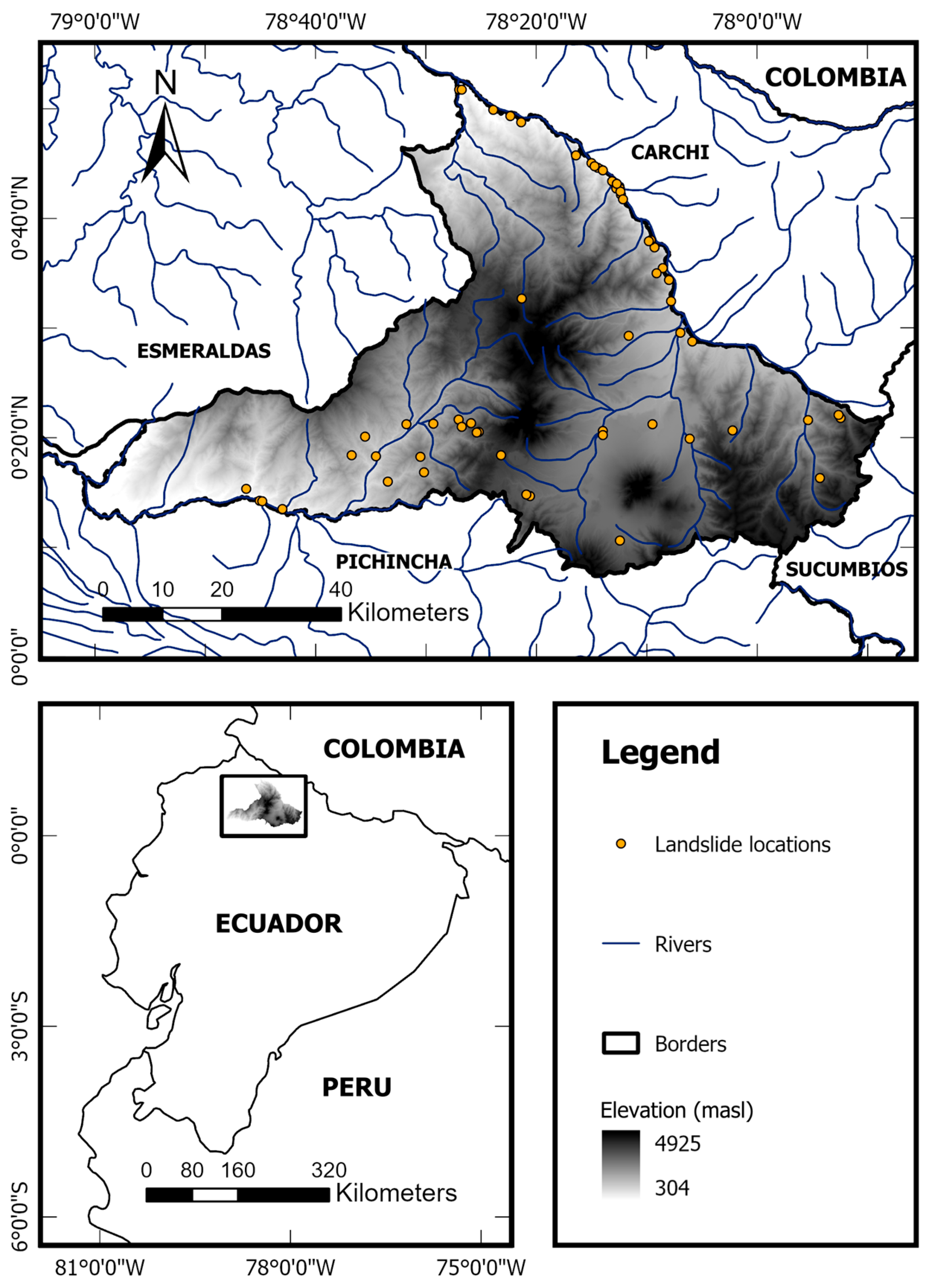
Figure 1. Study area with a topographic map showing landslide locations and river network.
Geohazards 07 00108 g001
Figure 2. Monthly Precipitation Anomaly distribution density showing the median value of 0.6 (red dashed line).
Geohazards 07 00108 g002
Figure 3. Landslide occurrence counts associated with recategorized geological (top), land use (middle) and vegetation cover (bottom) types (C&P: conservation and protection).
Geohazards 07 00108 g003
Figure 4. Histograms and density plots of topographic (ae,g,h) and precipitation (f) attribute variables. The black dashed line represents mean attribute values. Units on the axes.
Geohazards 07 00108 g004
Figure 5. Partial effects of the set of predictors on the log-odds of landslide occurrence for the selected GLM. Gray shadow shows 95% confidence intervals for continuous variables. Black lines represent standard errors with 95% confidence interval for categorical variables. Dashes on the x-axis are observations.
Geohazards 07 00108 g005
Figure 6. Predictive performance of the selected GLM (a) and GAM (b). ROC curves showing false positive rate (FPR) vs. true positive rate (TPR). The 45-degree dashed line represents a no-discrimination model.
Geohazards 07 00108 g006
Figure 7. Partial effects of transform functions of the selected GAM without interaction term. Gray shadow shows 95% confidence intervals for continuous variables. Black lines represent standard errors with 95% confidence intervals of fitted values (blue dots) for categorical variables. Dashes on the x-axis are observations.
Geohazards 07 00108 g007
Table 1. Cartographic information of the datasets obtained and produced for this study.
DatasetFormatYearScaleDescriptionSource
Geologic coverVector20051:100,000LithologyMAG 1
Vegetation coverVector19901:250,000Vegetation typesMAG 1
Land useVectorn.d.1:250,000Anthropogenic activitiesMAG 1
DEMRaster20181:80,000Digital elevation modelJAXA 2
SlopeRaster20181:80,000Slope anglesAuthors
AspectRaster20181:80,000Aspect anglesAuthors
CurvatureRaster20181:80,000CurvatureAuthors
Curvature plane and profileRaster20181:80,000Curvature planeAuthors
Catchment areaVector20181:80,000Drainage areaAuthors
Slope AspectRaster20181:80,000Compass direction Authors
1 Ministerio de Agricultura y Ganadería. 2 Japan Aerospace Exploration Agency.
Table 2. Vegetation cover and land use associated with landslide occurrence records.
DatasetCategoryLandslide Occurrence
No (0)Yes (1)
Vegetation cover (initial dataset)Corn orchards30
Crops of tempered zones20
Dry scrubland96
Humid forest54
Orchards01
Paramo vegetation10
Pasture crop forest716
Sugar cane crops10
Wet scrubland10
Vegetation cover after reclassificationHumid forest54
Orchards 51
Pasture crop forest615
Scrubland106
Land use (initial dataset)Agriculture97
Agriculture (C&P)31
Agric. and Livestock52
Forest (C&P)35
Livestock611
Livestock (C&P)10
Shrubby and herbaceous vegetation20
Wasteland01
Land use after reclassificationAgriculture128
Agric. and Livestock52
Forest (C&P)35
Livestock611
Bold letters indicate problematic categories in both vegetation cover and land use variables.
Table 3. Summary statistics of topographic and precipitation attribute variables.
Attributes [Units]MeanStandard DeviationMinMax
Elevation [masl]1727.07804.705693390
Slope [°]24.7111.775.2847.66
Curvature profile [0.01 m−1]0.090.96−1.821.936
Curvature plan [0.01 m−1]−0.080.82−1.603.21
log10 of Catchment area [log10 m2]3.620.892.817.14
Sine of the slope aspect [-]0.040.73−0.990.98
Cosine of the slope aspect [-]0.070.66−0.990.99
Monthly total precipitation [mm]142.8584.9820.50467.53
Table 4. Parameter estimates from the logistic regression model used to predict rainfall-related landslide occurrence. Estimated coefficients, odds ratios, and 95% confidence intervals are reported for all predictors included in the GLM. Blue-highlighted variables indicate predictors significant at the 5% level, whereas orange-highlighted variables indicate marginal significance at the 10% level. Significance was assessed under the null hypothesis that each predictor has no effect on the probability of landslide occurrence.
Predictor VariablesEstimateStd. Errorz ValuePr (>|z|)Exp (Estimates)2.50%97.50%
(Intercept)2.451.931.270.201.15 × 1013.32 × 10−11.41 × 10³
Land use: Agriculture and Livestock−10.575.31−1.990.052.56 × 1051.03 × 10−115.70 × 10⁻²
Land use: Forest (C&P)−7.144.32−1.650.107.95 × 10−43.15 × 10−95.66 × 10−1
Land use: Livestock4.483.631.230.228.83 × 1014.36 × 10−14.63 × 10⁶
Veg cover: Orchards−4.373.78−1.160.251.27 × 10−21.04 × 10−68.10
Veg cover: Pasture crop forest1.982.140.930.357.271.84 × 10−13.31 × 10³
Vege cover: Scrubland−1.472.68−0.550.582.30 ×10−16.42 × 10−43.93 × 101
Elevation7.644.061.880.062.09 × 1031.00 × 1014.30 × 108
Slope, 2nd degree, 15.205.550.940.351.81 × 1023.71 × 10−36.20 × 10⁷
Slope, 2nd degree, 211.455.811.970.059.38 × 1046.442.47 × 1011
Curvature profile, 3rd degree, 1−0.127.15−0.020.998.88 × 10−15.74 × 10−99.40 × 105
Curvature profile, 3rd degree, 2−6.346.49−0.980.331.76 × 10−33.03 × 10−111.19 × 10²
Curvature profile, 3rd degree, 316.4510.751.530.131.39 x 1073.111.13 × 1021
Curvature plan−0.240.89−0.260.797.90 × 10−19.26 × 10−24.18
Log 10 catchment area2.562.161.190.241.29 × 1013.53 × 10−14.57 × 10³
Sine of the slope aspect0.680.740.910.361.975.57 × 10−11.42 × 101
Cosine of the slope aspect1.461.091.340.184.317.43 × 10−19.59 × 101
Precipitation8.844.362.030.046.91 × 1032.68 × 1015.52 × 109
Table 5. Deviance-based comparison of candidate generalized additive models for rainfall-related landslide occurrence. The bolded row indicates the chosen model.
Generalized Additive Models
Model 1: Y ~ VegetationCover + LandUse + s(Elevation) + Slope + CurvatureProfile + CurvaturePlan + s(log10CatchmentArea) + s(SineSlopeAspect) + CosineSlopeAspect + Precipitation
Model 2: Y ~ VegetationCover + LandUse + s(Elevation) + Slope + s(CurvatureProfile) + CurvaturePlan + log10CatchmentArea + SineSlopeAspect + CosineSlopeAspect + Precipitation
Model 3: Y ~ VegetationCover + LandUse + s(Elevation) + s(Slope) + s(CurvatureProfile) +
CurvaturePlan + log10CatchmentArea + SineSlopeAspect + CosineSlopeAspect + Precipitation
ModelResid. DfResid. DevDfDeviancePr (>Chi)
136.09628.96
235.92719.0140.168239.94610.0001206
336.90419.275−0.97687−0.26090.5997967
Table 6. Parameter estimates of the selected GAM for the prediction of the probability of rainfall-related landslide occurrence using all 11 predictors. Blue-highlighted variables indicate predictors significant at the 5% level, whereas orange-highlighted variables indicate marginal significance at the 10% level. Significance was assessed under the null hypothesis that each predictor has no effect on the probability of landslide occurrence.
Predictor VariablesEstimateStd. Errorz ValuePr (>|z|)Exp (Estimates)
(Intercept)−7.424.23−1.760.085.97 × 10−4
Veg cover: Orchards1.854.850.380.706.36
Veg cover: Pasture crop forest11.506.281.830.079.88 × 104
Vege cover: Scrubland6.674.701.420.167.91 × 102
Land use: Agriculture and Livestock−18.1124.47−0.740.461.36 × 10−8
Land use: Forest (C&P)−5.003.22−1.550.126.75 × 10−3
Land use: Livestock5.793.901.490.143.29 × 102
Slope0.421.040.400.691.52
Curvature plan−2.261.79−1.260.211.05 × 10−1
Log 10 catchment area, poly3, 3−0.452.15−0.210.836.36 × 10−1
Sine of the slope aspect2.941.901.550.121.90 × 101
Cosine of the slope aspect4.372.621.670.107.94 × 101
Precipitation15.847.282.180.037.55 × 106
edfRef. edfChi.sqp-ValueExp (Estimates)
s (Elevation)1.9124.400.0956.76
s (Curvature profile)0.9523.300.0522.58
Disclaimer/Publisher’s Note: The statements, opinions and data contained in all publications are solely those of the individual author(s) and contributor(s) and not of MDPI and/or the editor(s). MDPI and/or the editor(s) disclaim responsibility for any injury to people or property resulting from any ideas, methods, instructions or products referred to in the content.