An Investigation to Detect Banking Malware Network Communication Traffic Using Machine Learning Techniques

Abstract

Banking malware are malicious programs that attempt to steal confidential information, such as banking authentication credentials, from users. Zeus is one of the most widespread banking malware variants ever discovered. Since the Zeus source code was leaked, many other variants of Zeus have emerged, and tools such as anti-malware programs exist that can detect Zeus; however, these have limitations. Anti-malware programs need to be regularly updated to recognise Zeus, and the signatures or patterns can only be made available when the malware has been seen. This limits the capability of these anti-malware products because they are unable to detect unseen malware variants, and furthermore, malicious users are developing malware that seeks to evade signature-based anti-malware programs. In this paper, a methodology is proposed for detecting Zeus malware network traffic flows by using machine learning (ML) binary classification algorithms. This research explores and compares several ML algorithms to determine the algorithm best suited for this problem and then uses these algorithms to conduct further experiments to determine the minimum number of features that could be used for detecting the Zeus malware. This research also explores the suitability of these features when used to detect both older and newer versions of Zeus as well as when used to detect additional variants of the Zeus malware. This will help researchers understand which network flow features could be used for detecting Zeus and whether these features will work across multiple versions and variants of the Zeus malware.

1. Introduction

Cybercrime is a major threat to cybersecurity [1,2] estimates that the yearly cost of cybercrime could rise to USD 10.5 trillion by the year 2025 and a significant proportion of this is related to malware such as banking malware. Banking malware have also been increasing on a yearly basis, and according to [3], banking malware attacks have increased by 80% in 2021 alone. One of these banking variants, specifically, the Zeus malware (from hereon, referred to as Zeus), has become one of the most prevalent banking malware variants ever discovered [4]. Furthermore, in 2011, the Zeus program code was made public [5], allowing malware developers to create additional variants of Zeus and to also develop additional modules for the Zeus malware [6]. Since the Zeus code was leaked, many variants of Zeus have emerged, and some of these include ZeusPanda, Ramnit and Citadel.

1.1. Need for Malware Detection

As the number of malware and their variants are increasing rapidly and becoming more sophisticated and prevalent [7], additional modern techniques need to be developed to detect these malware variants, and [7] highlights the importance of using AI to detect malware. The authors of [8] also discuss the limitations in other malware detection approaches, such as detecting malicious patterns in executables, and using heuristic-based approaches and statistical approaches and have recommended that researchers should use machine learning and deep learning approaches to address these limitations. Signature-based malware detection systems also exist, but these systems also have limitations; for example, they can only detect known malware [9].

This paper proposes a framework and methodology to detect malware and benign traffic using machine learning and deep learning algorithms. The main contributions of this paper are to develop a methodology to detect the Zeus banking malware and differentiate it from benign traffic using binary classification machine learning algorithms. This paper will compare three binary classification algorithms to determine which provides the best detection results when used to detect Zeus from benign traffic. This paper also determines the minimum number of features that could be used to detect Zeus and benign traffic. Researchers [10,11,12,13] have discussed and proposed several supervised machine learning (ML) algorithms that could be used for analysing this type of problem and this paper uses three of these ML algorithms. These are: random forest ML algorithm, decision tree ML algorithm and the KNN deep learning algorithm. This paper aims to:

• Determine a methodology that can be used by deep learning and machine learning algorithms for detecting the Zeus malware.
• Determine which ML algorithm produces the best detection results.
• Determine whether the features that produce the best detection results on one dataset will work on other datasets from other sources.
• Determine a minimum set of features that could be used for detecting Zeus.
• Determine whether the features that produce the best detection results work across newer and older versions of Zeus.
• Determine whether the features that produce the best detection results when detecting Zeus also work on additional variants of the Zeus malware.

1.2. Zeus Malware Architecture

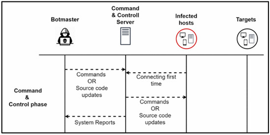
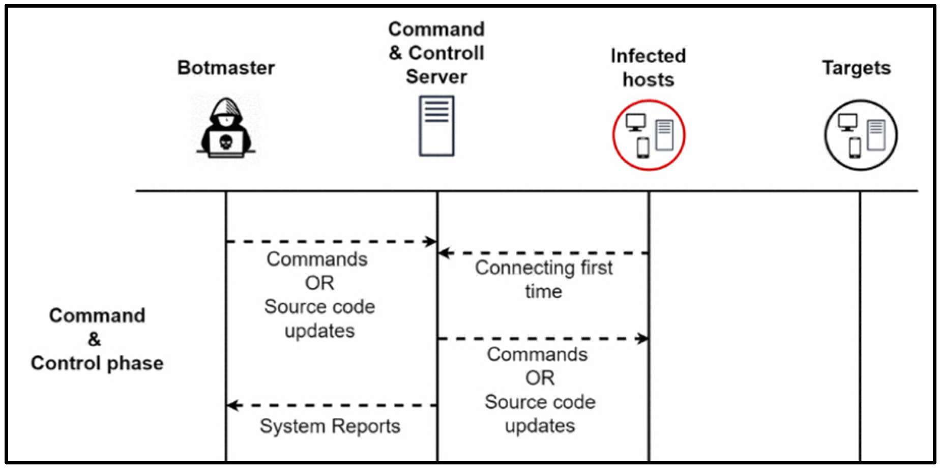
An important feature of the Zeus malware is the way that it communicates, as it uses command and control channels (C&C) for this purpose. The author of [14] has discussed the various phases of the C&C communication, which can be seen in Figure 1. This communication can occur using either a centralised or a peer-to-peer architecture, with the peer-to-peer architecture being more robust and resilient [15]. This is because if the central C&C server becomes unreachable or is taken down, the Zeus bots will not be able to communicate with the C&C server, preventing the bots from receiving commands, updating themselves and downloading new configuration files [16]. Newer variants of Zeus use the P2P C&C architecture. These are more resilient to takedown efforts because the configuration file does not point to a static C&C server [17]. Instead, the C&C server information is obtained from a peer (proxy bot), which can be updated if the C&C server is taken down or becomes unreachable [18]. Stolen data is routed through the C&C network to the malware authors’ C&C server, where the stolen data is decrypted and saved to a database [19].

Figure 1. C&C Communication phases.

As discussed by [20], Zeus propagates like a virus, mainly infecting Windows systems and predominantly, the infection vector occurs via phishing emails, which is a significant distribution mechanism for malware. Research by [21] has discussed this in detail, and states that around 90 percent of data breaches are caused by phishing. Once the Zeus binary executes on a Windows system, it performs several actions. One of these is to create two files called local.ds and user.ds. Local.ds is the dynamic configuration of the file downloaded from the command and control (C&C) server, while the user.ds stores stolen credentials and other information that needs to be transmitted back to the C&C server [22]. Additional code is injected into svchost and is responsible for network communications. Svchost is also responsible for injecting malicious code into many Windows processes, which provide Zeus with the ability to steal credentials and launch financial attacks.

2. Related Studies

Bothunter [23] is a perimeter scanning system which uses three sensors and a correlation engine to identify malicious traffic flows that can occur between an infected host and a malicious entity. Bothunter [23] has been built on top of the open-source platform called SNORT, and it is an application developed to track the various stages of the malware communication flow and can correlate both inbound and outbound traffic to identify malware traffic. Two plugins called SLADE and SCADE are used by Bothunter, and SCADEs role is to analyse the communication flows to identify traffic patterns that can be considered harmful. These traffic patterns include:

• Hosts that frequently scan external IP addresses.
• Outbound connection failures.
• An evenly distributed communication pattern which is likely to indicate that that communication is malicious.

SLADEs role is to analyse network packets and alert the administrator if a packet deviates from an established profile. SLADE was developed using PAYL [24], which allows SLADE to examine 256 features of the packet and then use this information to make determinations as to whether the packet is malicious or not.

Botminer [25] is a tool that was designed to detect groups of compromised computers, and this is achieved by monitoring network communication flows using two modules, a C-plane module, and an A-plane module. The C-plane’s role is to log network traffic to identify all the hosts that are communicating, and the A-plane’s role is to identify what these hosts are doing. Features extracted from both these modules can be used to identify communication patterns that are similar between hosts and if these communication patterns are malicious, it is indicative that a particular group of hosts are communicating maliciously. The A-plane module is based on Bothunter’s [23] SCADE module and can analyse communications to determine malicious communication patterns [25].

CONIFA [26] uses machine learning to detect malware communication traffic, and it does this by training and testing the Zeus malware by using the correlation-based feature selection (CFS) algorithm with the C4.5 classification algorithm. To improve CONIFAs accuracy and prediction results, [26] created a cost-sensitive variant of the C4.5 classification algorithm, which uses a lenient and strict classifier and compares the prediction results to a standard machine learning framework, which uses a cost-insensitive version of the C4.5 algorithm. The standard framework’s detection rate was good when evaluating the training dataset; however, when evaluating the test data, the recall rate dropped to 56%. CONIFAs results demonstrated an improvement in the detection accuracy, with the recall rate increasing to 67%.

The RCC Detector (RCC) [27] analyses network traffic flowing from a host to identify any malware communication traffic. To do this, the RCC [27] uses a multi-layer perceptron (MLP) and a temporal persistence (TP) classifier. The MLP classifier is made up of an input layer, an output layer and one hidden layer [27], and these are used to classify botnets using several characteristics, including, the Flow count, session length, uniformity score and the Kolmogorov–Smirnov Test.

The multi-layer feed forward network (MLFFN) [28] is a tool that extracts TCP features from the TCP connections originating from a host computer and uses these to identify botnet communication traffic. MLFFN [28] consists of an input layer made up of six neurons and an output layer made up of four neurons. MLFFN was tested on four datasets, namely, Zeus-1, Zeus-2, Spyeye-1 and Spyeye-2, and it is worth noting that these are all older versions of the Zeus malware.

Genetic programming (GP) [29] used the Symbiotic Bid-Based (SBB) algorithm and the C4.5 machine learning algorithms to identify unique botnet communication patterns, and to do this, features were extracted from the communication flows of three malware variants including Zeus, Conficker and Torpig. The features were extracted using Softflowd [30], and the authors of [29] were able to categorise these three malware variants. It is worth noting that the results are based the usage of the older versions of the malware variants.

MOCA [31] uses a two-stage monitoring and classification system to detect and classify malicious attacks. It does this by identifying behaviours within the network flows that are outside of the normal range (abnormal) and this part of the MOCA system is classed as the stage one classifier of the MOCA system. These abnormal behaviours are then sent to the stage two classifier, which attempts to classify the attacks into a class such as a DDoS attack in an IoT network or a Botnet attack. Two datasets were used for testing, CICIDS2017 and CICDDOS2019, and the accuracy achieved was 99.84% for CICIDS2017 and 93% for the CICDDOS2019 dataset. The algorithms used in this research include the decision tree, random forest and XGBoost ML algorithms.

3. Problem Statement

This paper intends to develop a framework and methodology that uses machine learning techniques to detect malware. Other methodologies exist and have been used by many researchers to detect malware. These include anomaly-based detection approaches such as those discussed by [32,33], and signature-based approaches such as those discussed by [34,35]; however, these do have drawbacks, and these are highlighted in [36]. For example, signature based-systems need to be updated regularly to cater for newly emerging malware variants, and signature-based systems are not able to detect unknown malware variants or zero-day malware.

Machine learning can help address many of these issues [37] and this paper has developed a framework and approach using machine learning that will be able to detect several banking malware variants. Although other researchers [26,27,28] have done some experimental work on detecting malware, there is little to no research that aims to detect a range of malware variants by only training one dataset, i.e., one malware variant. This research paper aims to use only one dataset for training and then use this to build a machine learning model. This model is then used to detect multiple banking malware variants and is also used to distinguish between benign and malware communication traffic. This research is also analysing banking malware variants that have emerged recently and those that have been around since they were developed, and this should ensure that both the older and newer versions of the banking malware are detectable by the machine learning algorithms.

4. Research Methodology

This research paper aims to classify network traffic flows as either Zeus (malware) or benign (good). For this research, the raw network traffic samples were collected as pcap files, and each pcap file is made up of network flows, which refers to a sequence of packets flowing between a source and a destination host. In this paper, the flows are referred to as ML samples and the features are extracted from these samples.

4.1. Data Collection and Preperation

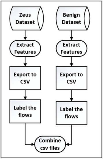
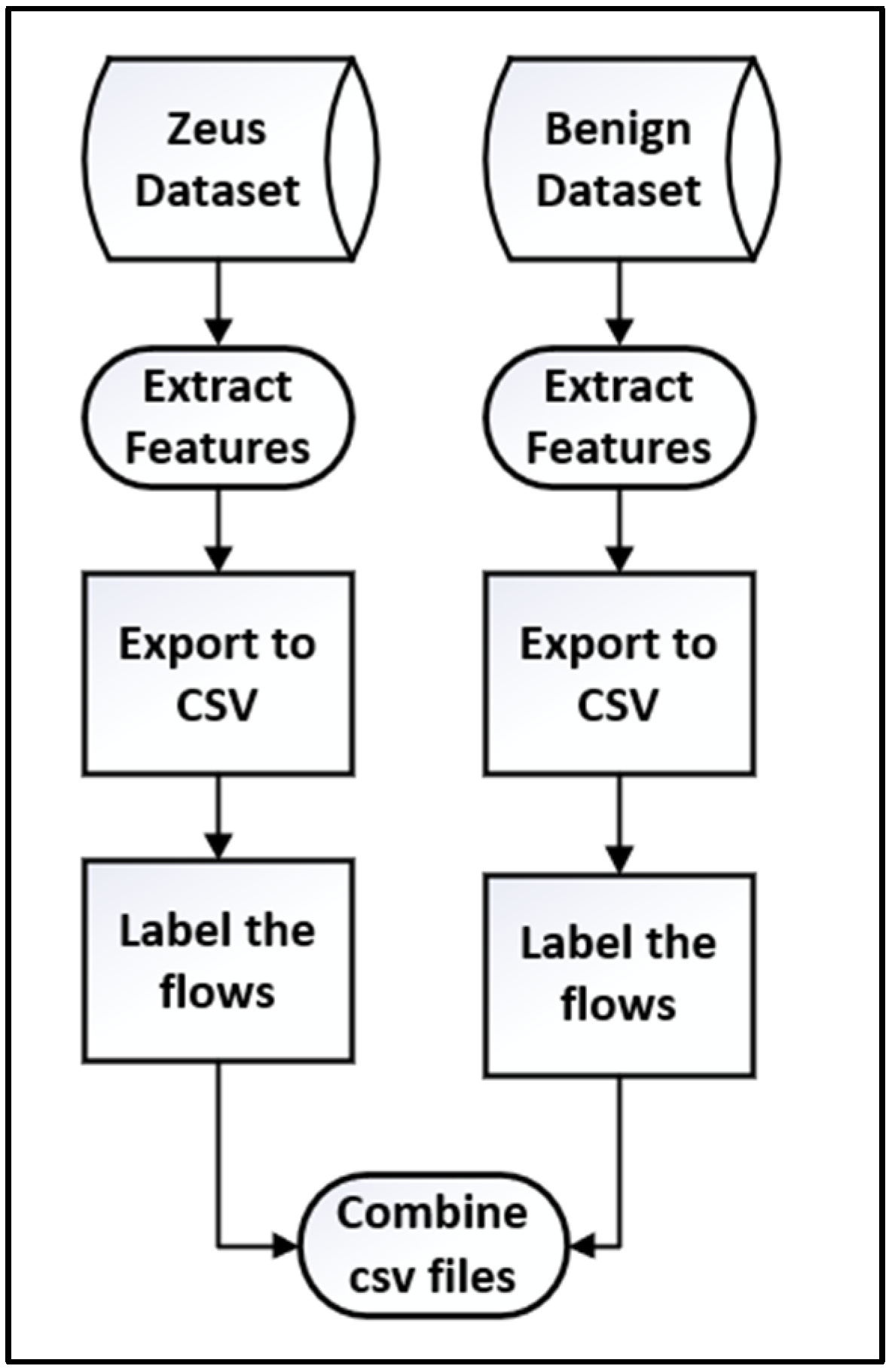
Figure 2 depicts the data collection and preparation steps and is discussed further in this section. To prepare the data for the ML algorithms, the features were extracted from the samples using Netmate-flowcalc (NF), a tool developed by [38], and were then exported into a CSV file. NF was used because it is an open-source tool that can extract the features required by the ML algorithms and has also been used by other researchers [39,40,41,42]. A total of 44 features were extracted by NF (see Appendix A for a brief description of the features), and the features from the benign and Zeus flows were extracted into separate CSV files and labelled. A label of ‘1’ was applied to the Zeus samples and a label of ‘0’ was applied to the benign samples. The two files were then combined into one CSV file, and this was used for the empirical analysis conducted during this research.

Figure 2. Methodology for collecting and preparing the data.

4.2. Feature Selection

One of the main issues in ML is selecting the appropriate features for the ML algorithm, and the criticality of this has been discussed by many researchers such as [43,44]. Selecting the right features has the following benefits:

• Variance (overfitting) is reduced.
• Computational cost and the time for running the algorithm is reduced.
• Enables the ML algorithm to learn faster.

There are several techniques that can be used for selecting the appropriate and best features and [45,46] discuss these in detail. For example, two of these techniques are:

• Filter method—Feature selection is independent of the ML algorithm.
• Wrapper method—A subset of the features are selected and used to train the ML algorithm. Based on the results, features are either removed or added until the best features are determined.

For this research, the features were studied [47,48,49,50] and based on this, the features were divided into two groups, called Feature set1 and Feature set2, and only the features from Feature set1 were used during this research. Feature set2 contained those features that were not used during this research and were excluded. This was because these features could potentially be related to the characteristics of the network from which the packets were extracted, resulting in the ML algorithm making false correlations. For example, if the benign and malware traffic came from a particular IP address range, the ML algorithm might use the IP address information to make predictions. Table 1 shows the features that were excluded (Feature set2). All the remaining features were included in Feature set1 and were used during this research. These features are: total_fpackets, total_fvolume, total_bpackets, total_bvolume, min_fpktl, mean_fpktl, max_fpktl, std_fpktl, min_bpktl, mean_bpktl, max_bpktl, std_bpktl, sflow_fpackets, sflow_fbytes, sflow_bpackets, sflow_bbytes, fpsh_cnt, bpsh_cnt, furg_cnt, burg_cnt, total_fhlen, total_bhlen, duration, min_active, mean_active, max_active, std_active, min_idle, mean_idle, max_idle and std_idle.

Table 1. The features that were not used during this research.

Feature That Was Removed	Justification
srcip	This is the source IP which was removed to negate any correlation with a network characteristic
srcport	The is the source port number which was removed to negate any correlation with a network characteristic
dstip	This is the destination IP address which was removed to negate any correlation with a network characteristic
dstport	The is the destination port number which was removed to negate any correlation with a network characteristic
proto	This is the protocol that was being used (i.e., TCP = 6, UDP = 17) which was removed to negate any correlation with a network characteristic
min_fiat	This is the minimum time between two packets sent in the forward direction (in microseconds) which was removed to negate any correlation with a network characteristic
mean_fiat	This is the mean amount of time between two packets sent in the forward direction (in microseconds) which was removed to negate any correlation with a network characteristic
max_fiat	This is the maximum time between two packets sent in the forward direction (in microseconds) which was removed to negate any correlation with a network characteristic
std_fiat	This is the standard deviation from the mean time between two packets sent in the forward direction (in microseconds)
min_biat	This is the minimum time between two packets sent in the backward direction (in microseconds) which was removed to negate any correlation with a network characteristic
mean_biat	This is the mean time between two packets sent in the backward direction (in microseconds) which was removed to negate any correlation with a network characteristic
std_biat	This is the standard deviation from the mean time between two packets sent in the backward direction (in microseconds) which was removed to negate any correlation with a network characteristic

4.3. Datasets (Samples)

This paper analyses and compares the performance of the ML algorithms using nine datasets obtained from four locations. One location was Zeustracker [51], a website that monitors Zeus C&C activities, and these samples were downloaded on 4 February 2019. The other datasets were obtained from Stratosphere, Abuse.ch and Dalhousie University, and these datasets are a combination of older and newer versions of the Zeus malware and three other variants of the Zeus malware, which are ZeusPanda, Ramnit and Citadel. Stratosphere [52] specializes in collecting malware and benign traffic captures, and they have multiple datasets which have been made available for research purposes. Abuse.ch is a research project that identifies and tracks malware and botnets, and is a platform integrated with many commercial and open-source platforms, including VirusTotal, ClamAV, Karspersky and Avast [53]. Dalhousie University has botnet samples that are available for download and these samples are part of the NIMS botnet research dataset and have been used by other researchers [54]. Table 2 describes the datasets that were used for the research reported in this paper.

Table 2. Datasets used in this research.

Dataset Type	Malware Name/Year	Number of Flows	Name of Dataset for This Paper
Malware Benign	Zeus/2022	272,425	Dataset1
	N/A	272,425
Malware Benign	Zeus/2019	66,009	Dataset2
	N/A	66,009
Malware Benign	Zeus/2019	38,282	Dataset3
	N/A	38,282
Malware Benign	Zeus/2014	200,000	Dataset4
	N/A	200,000
Malware Benign	Zeus/2014	35,054	Dataset5
	N/A	35,054
Malware Benign	Zeus/2014	6049	Dataset6
	N/A	6049
Malware Benign	ZeusPanda/2022	11,864	Dataset7
	N/A	11,864
Malware Benign	Ramnit/2022	10,204	Dataset8
	N/A	10,204
Malware Benign	Citadel/2022	7152	Dataset9
	N/A	7152

4.4. Machine Learning Algorithms

The ML algorithms used for this research are discussed in this section, and they are supervised machine learning algorithms as these are used and are the most suitable for classification problems, as discussed by [55]. The machine learning algorithms used during this research include the decision tree (DT) algorithm, the random forest (RF) algorithm and the keras neural network (KNN) deep learning algorithm.

The decision tree algorithm is a common machine learning algorithm that can be used for classification problems [56] and is especially useful when used for binary classification problems [56]. For this reason, the decision tree algorithm is well suited for this prediction problem because this analysis is trying to determine if the network flow is malicious (Zeus banking malware traffic), or benign. The authors of [57] also state that the decision tree algorithm can produce good prediction results.

The random forest (RF) algorithm works by building and combining multiple decision trees [58]. It can be more efficient and provide better prediction results than the decision tree algorithm [59], and it reduces the possibility of overfitting [60]. It is important to tune the parameters to try and increase the prediction accuracy when using the RF algorithm; however, it is difficult to predict the best parameters ahead of time as the parameters are selected based on trial and error. One of these parameters is the number of trees built during the training and testing of the data. The author of [61] states that building more than 128 trees provides no significant gain in the accuracy and can increase costs. The authors of [61] also state that the optimum number of trees for the random forest classifier was found to be between 64 and 128. For this empirical analysis, the random forest algorithm was coded to build between 64 and 128 decision trees, and once the training was complete, the optimal number of trees was selected based on the best prediction results.

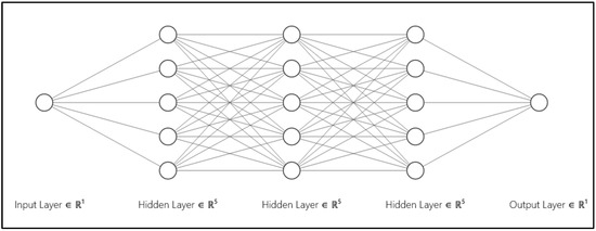
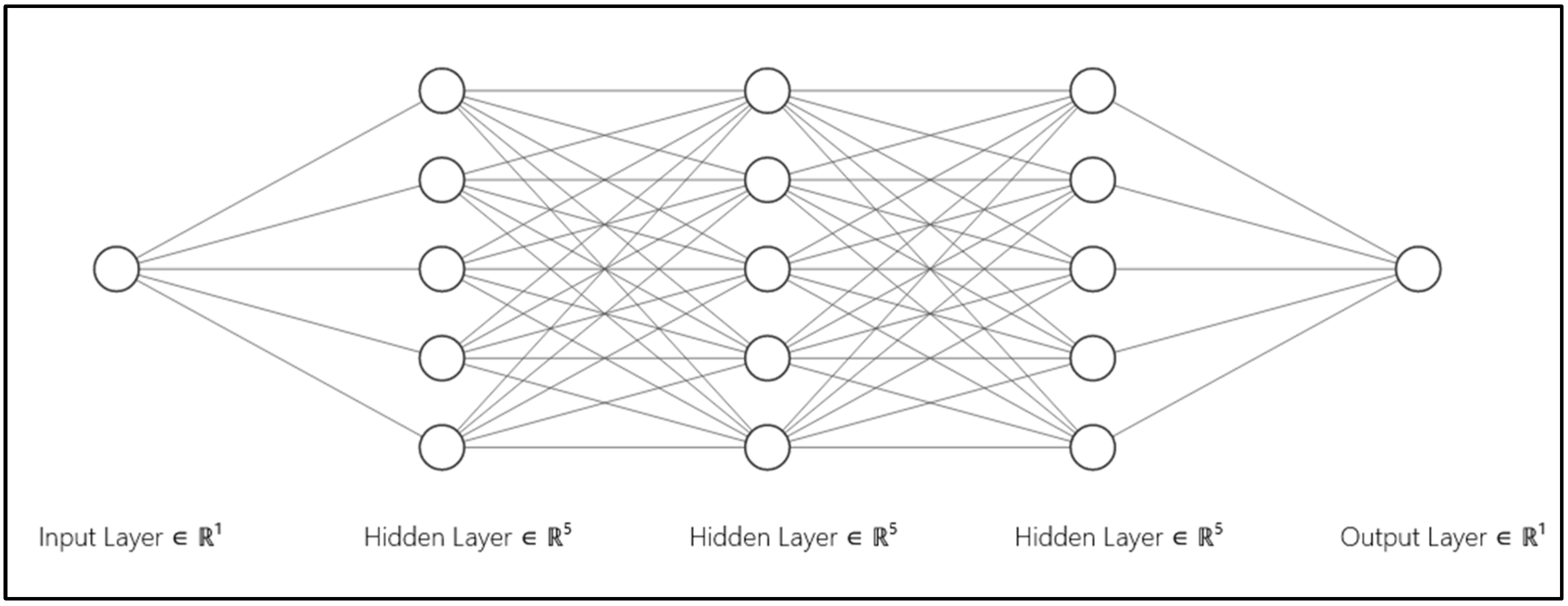
Keras is a popular neural network library implemented in Python [62] and can be used for classification problems such as the one examined during this research [63]. The keras neural network (KNN) deep learning algorithm was used for training and testing the datasets and for this empirical analysis, a sequential KNN model [64] was used, which means that the output of one layer is input into the next layer. For this research, the deep learning model consisted of one input layer, three hidden layers and one output layer, and a graphical representation of this can be seen in Figure 3. It is important to note that only one of the datasets was used for training and the remaining datasets were used for testing.

Figure 3. A neural network.

4.5. System Architecture and Methodology

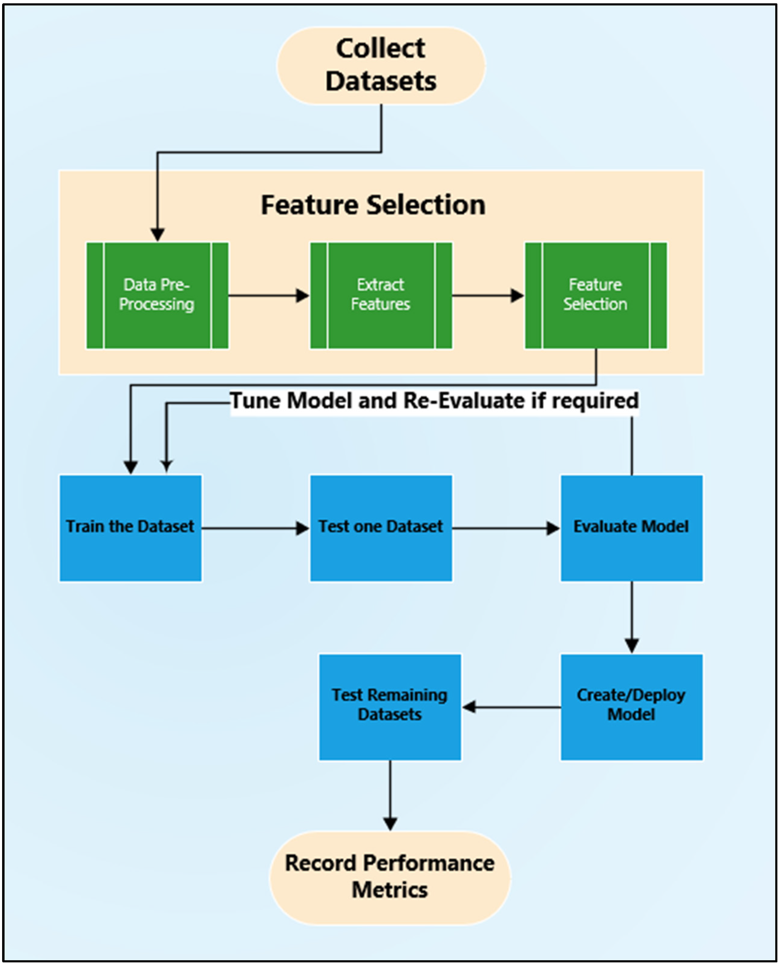
The system architecture is depicted in Figure 4 and shows the steps that are completed to prepare the samples for the ML algorithms. These include:

• The datasets are identified and collected.
• Features are extracted from these datasets.
• The extracted features are transferred to a CSV file and prepared.
• The features are selected for training and testing.
• The algorithm is trained and tested, and a model is created. Only one dataset is used for the training.
• The model is tuned and trained and tested again if required.
• The model is used to test and evaluate the remaining datasets.
• Deploy the final model, test all the data samples and create a report highlighting the evaluation metrics.

Figure 4. System Design.

Figure 4. System Design.

4.6. Evaluation

Precision, recall and f1-score evaluation metrics [65] are used to determine the accuracy of the ML algorithms. Precision is the percentage of correctly identified positive cases from the whole data sample, which in this case is the malware and benign samples [65]. Recall is the percentage of correctly identified positive cases from the positive samples only [66], which in this case is the malware samples. The formulas to calculate precision and recall are:

$$Precision=\frac{TP}{TP+FP}$$

(1)

$$Recall=\frac{TP}{TP+FN}$$

(2)

The f1-score is another measure used for evaluation, and this considers both the positive and negative cases. The author of [67] states that the precision and recall are both combined during the evaluation of the ML algorithm. The formula to calculate the f1-Score is set out below:

$$F1-Score=\frac{2\times \left(Precision\ast Recall\right)}{Trecisio+Recall}$$

(3)

A confusion matrix [67] will also be generated, and an example of this is shown in Table 3. The confusion matrix will be used to measure the performance and prediction accuracy of the algorithm when tested and evaluated on the unseen datasets, and it will identify how many Zeus and benign samples were correctly identified.

Table 3. An example of the confusion matrix used to measure the detection accuracy.

	Predicted Benign	Predicted Zeus
Actual Benign (Total)	TN	FN
Actual Zeus (Total)	FP	TP

5. Results

This section presents the training and testing results of the three algorithms and compares the prediction results.

5.1. Training and Testing the Machine Learning Algorithms Using the Data Sets

The DT and RF algorithms were trained on Dataset1, using all the features from Feature set1, and a model was created and used for testing all the remaining datasets. The precision, recall and f1-score results for the DT algorithm can be seen in Table 4, and the precision, recall and f1-score results for the RF algorithm can be seen in Table 5. A confusion matrix was generated for testing all the datasets and the results of these can be seen in Table 6 and Table 7. They also show the number of Zeus samples tested, how many of the Zeus samples were correctly classified (true positives) and how many of the Zeus samples were misclassified (false negatives). The table also shows the number of benign samples tested, how many of these were classified correctly (true negatives) and how many of these were misclassified (false positives).

Table 4. Test results when using the decision tree algorithm.

Dataset Name	Benign Precision Score	Benign Recall Score	Benign f1-Score	Malware Precision Score	Malware Recall Score	Malware f1-Score
Dataset1	0.99	1	0.99	1	0.99	0.99
Dataset2	0.94	1	0.97	1	0.94	0.97
Dataset3	0.95	1	0.97	1	0.94	0.97
Dataset4	0.71	0.87	0.78	0.83	0.64	0.72
Dataset5	0.67	1	0.8	1	0.52	0.68
Dataset6	0.62	1	0.76	1	0.39	0.56
Dataset7	0.99	1	0.99	1	0.99	0.99
Dataset8	0.98	0.87	0.92	0.88	0.98	0.93
Dataset9	0.96	1	0.98	1	0.96	0.98

Table 5. Test results when using the random forest algorithm.

Dataset Name	Benign Precision Score	Benign Recall Score	Benign f1-Score	Malware Precision Score	Malware Recall Score	Malware f1-Score
Dataset1	1	1	1	1	1	1
Dataset2	0.98	1	0.99	1	0.98	0.99
Dataset3	0.98	1	0.99	1	0.98	0.99
Dataset4	0.75	0.89	0.82	0.86	0.71	0.78
Dataset5	0.8	1	0.89	1	0.74	0.85
Dataset6	0.68	1	0.81	1	0.53	0.69
Dataset7	0.99	1	0.99	1	0.99	0.99
Dataset8	0.94	0.88	0.91	0.89	0.94	0.92
Dataset9	0.95	1	0.98	1	0.95	0.97

Table 6. Confusion matrix for testing with the decision tree algorithm.

Dataset Name	Benign Precision Score	Benign Recall Score	Benign f1-Score	Malware Precision Score	Malware Recall Score	Malware f1-Score
Dataset1	272,425	271,721	704	272,425	270,109	2316
Dataset2	66,009	65,832	177	66,009	61,920	4089
Dataset3	38,222	38,127	95	38,282	36,061	2221
Dataset4	200,000	173,219	26781	200,000	127,706	72,294
Dataset5	35,054	34,963	91	35,054	18,116	16,938
Dataset6	6049	6040	9	6049	2333	3716
Dataset7	11,864	11,836	28	11,864	11,715	149
Dataset8	10,204	8865	1339	10,204	10,041	163
Dataset9	7152	7138	14	7152	6839	313

Table 7. Confusion matrix for testing with the random forest algorithm.

Dataset Name	Benign Precision Score	Benign Recall Score	Benign f1-Score	Malware Precision Score	Malware Recall Score	Malware f1-Score
Dataset1	272,425	272,200	225	272,425	271,312	1113
Dataset2	66,009	65,946	63	66,009	64,438	1571
Dataset3	38,282	38,252	30	38,282	37,546	736
Dataset4	200,000	177,309	22,691	200,000	142,286	57,714
Dataset5	35,054	35,025	29	35,054	26,104	8950
Dataset6	6049	6046	3	6049	3179	2870
Dataset7	11,864	11,852	12	11,864	11,740	124
Dataset8	10,204	9014	1190	10,204	9642	562
Dataset9	7152	7145	7	7152	6803	349

5.2. Training and Testing the Deep Learning Algorithm Using the Data Sets

The DL algorithm was also trained in a similar manner and the precision, recall and f1-score results can be seen in Table 8, and the confusion matrices can be seen in Table 9.

Table 8. Test results when using the deep learning algorithm.

Dataset Name	Benign Precision Score	Benign Recall Score	Benign f1-Score	Malware Precision Score	Malware Recall Score	Malware f1-Score
Dataset1	0.98	0.97	0.98	0.97	0.98	0.98
Dataset2	0.92	0.97	0.94	0.97	0.91	0.94
Dataset3	0.92	0.98	0.95	0.97	0.92	0.95
Dataset4	0.69	0.95	0.8	0.93	0.56	0.7
Dataset5	0.7	0.97	0.81	0.96	0.58	0.72
Dataset6	0.87	0.99	0.93	0.99	0.86	0.92
Dataset7	0.97	0.97	0.97	0.97	0.97	0.97
Dataset8	0.91	0.94	0.93	0.94	0.91	0.92
Dataset9	0.92	0.98	0.95	0.98	0.92	0.95

Table 9. Confusion matrix for using the deep learning algorithm.

Dataset Name	Benign Precision Score	Benign Recall Score	Benign f1-Score	Malware Precision Score	Malware Recall Score	Malware f1-Score
Dataset1	272,425	265,452	6973	272,425	266,091	6334
Dataset2	66,009	64,123	1886	66,009	60,310	5699
Dataset3	38,282	37,356	926	38,282	35,177	3105
Dataset4	200,000	190,935	9065	200,000	112,731	87,269
Dataset5	35,054	34,155	899	35,054	14,753	20,301
Dataset6	6049	5973	76	6049	5180	869
Dataset7	11,864	11,566	298	11,864	11,551	313
Dataset8	10,204	9605	599	10,204	9260	944
Dataset9	7152	7023	129	7152	6547	605

5.3. Comparing the Predication Results of the Three Algorithms Tested

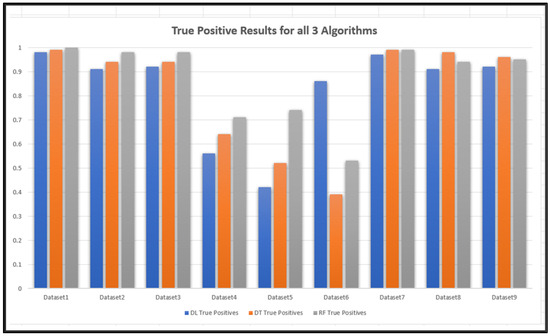
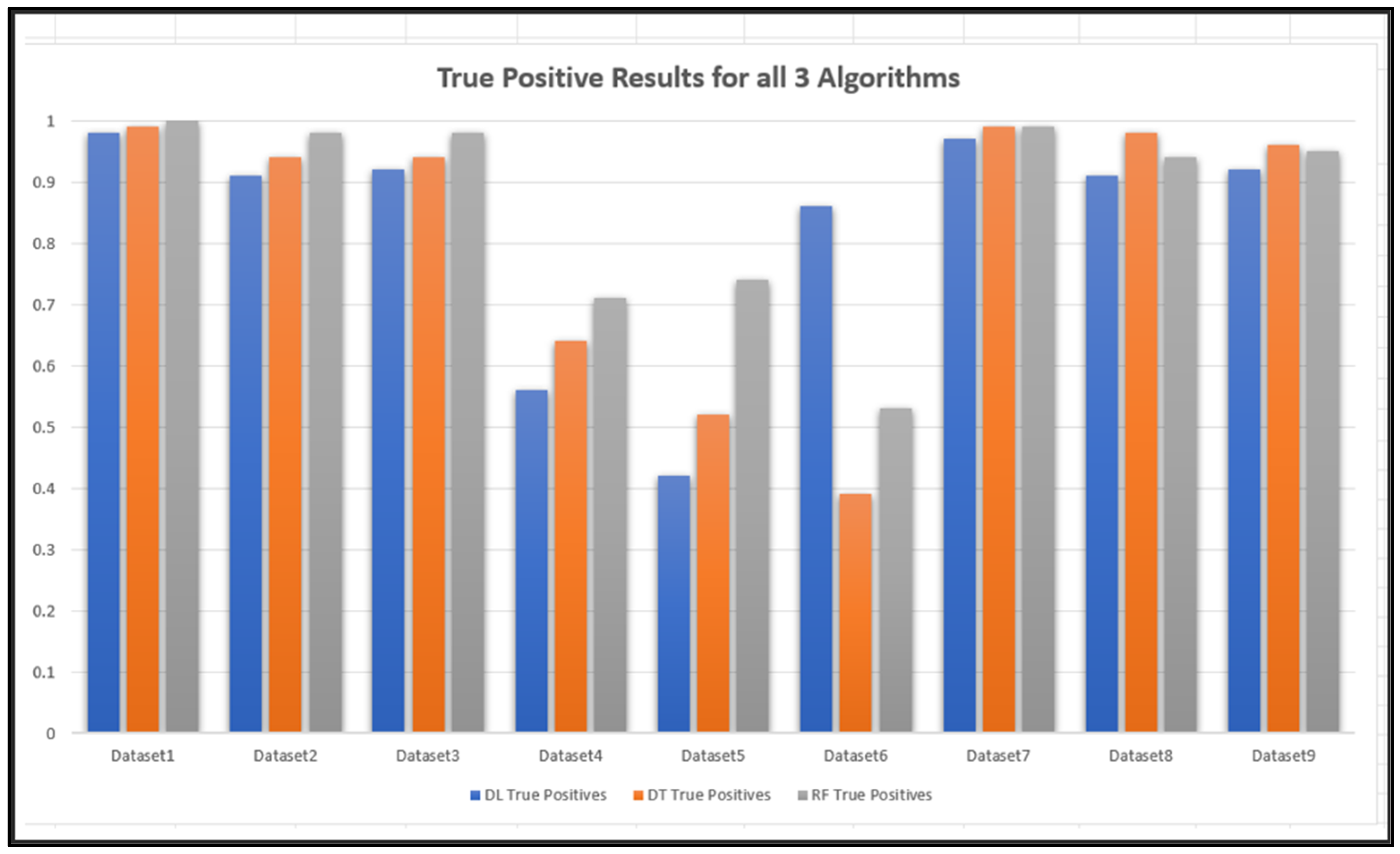
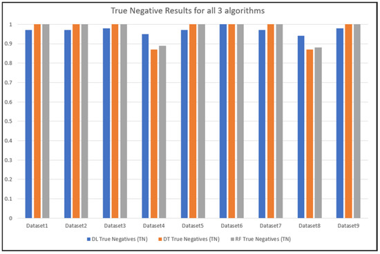
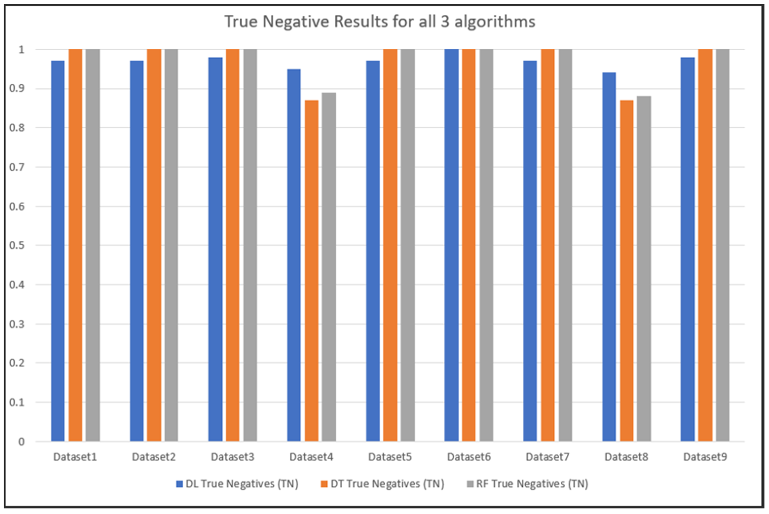
The results obtained from testing the three algorithms are all compared in this section. Figure 5 shows the true positive results of all the algorithms when tested against all the datasets, and Figure 6 shows the true negative results when tested against all the datasets.

Figure 5. Comparison of the Zeus prediction results for all three ML algorithms.

Figure 6. Comparison of the benign prediction results for all three ML algorithms.

The Zeus malware prediction accuracy for dataset1, dataset2, dataset3, dataset7, dataset8 and dataset9 were all above 90%, with the random forest algorithm performing the best with an average accuracy prediction result of 97% across these datasets. The three 2014 Zeus datasets (dataset4, dataset5 and dataset6) produced mixed results with the deep learning algorithm, performing better than the other two, with a detection result of 86% for dataset6. For dataset4 and dataset5, the random forest algorithm performed the best with a result of 71% and 74%, respectively.

For the benign traffic, the prediction results showed that for dataset1, dataset2, dataset3, dataset5, dataset6, dataset7, dataset8 and dataset9, the prediction accuracy for all the algorithms were above 90%, with the random forest algorithm performing the best with an average accuracy prediction result of 98% across these datasets. For dataset4 and dataset8, the deep learning algorithm performed best with a result of 95% and 94%, respectively, and the decision tree algorithm had the lowest prediction with a result of 87% for both these datasets.

This paper has demonstrated a methodology that could be used to detect the Zeus malware and its variants and has demonstrated that the methodology does work across multiple datasets and three other variants of the Zeus malware. The next section (Section 4.4) investigates the impact of the prediction accuracy when the number of features used during testing and training are reduced.

5.4. Reducing the Features to the Minimum Number of Possible Features

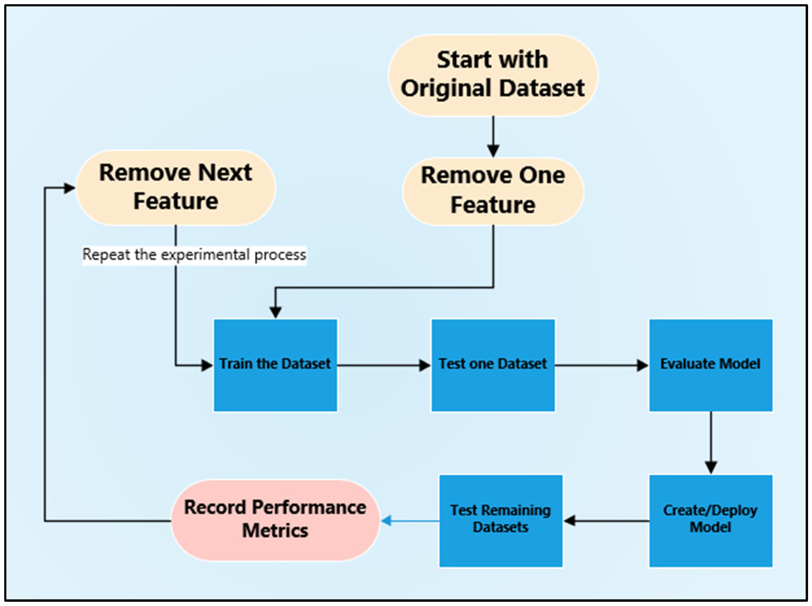
Multiple experiments were conducted by reducing the features from Feature set1 and this section seeks to investigate the prediction accuracy of both the malware and benign traffic as the number of features are reduced. To do this, the ML algorithms were trained and tested using dataset1, and the impact rating of each feature was determined and then used to establish which features have the highest impact ratings and which features have the lowest impact ratings. Some of these impact ratings can be seen in Figure 7. For example, Figure 7 shows that the mean active feature has an impact rating of 13.103% and that max_bpktl has an impact rating of 6.025%. Analysing the features in this way supported the systematic removal of the features, and this process can be seen in Figure 8. This process is described here.

• Remove one feature which has the lowest impact score.
• Training a dataset with this one feature redacted.
• Test the remaining datasets.
• Calculate the prediction accuracy and record the results.
• Remove another feature and re-train the dataset.
• Test the remaining datasets.
• Calculate the prediction accuracy and record these results.
• Repeat this process until the accuracy of two of the datasets fall below 50% during testing, as this would mean that more than half of the Zeus samples were misclassified for two or more of the datasets.

Figure 7. Feature impact scores.

Figure 7. Feature impact scores.

Figure 8. Flow diagram showing the feature redaction process.

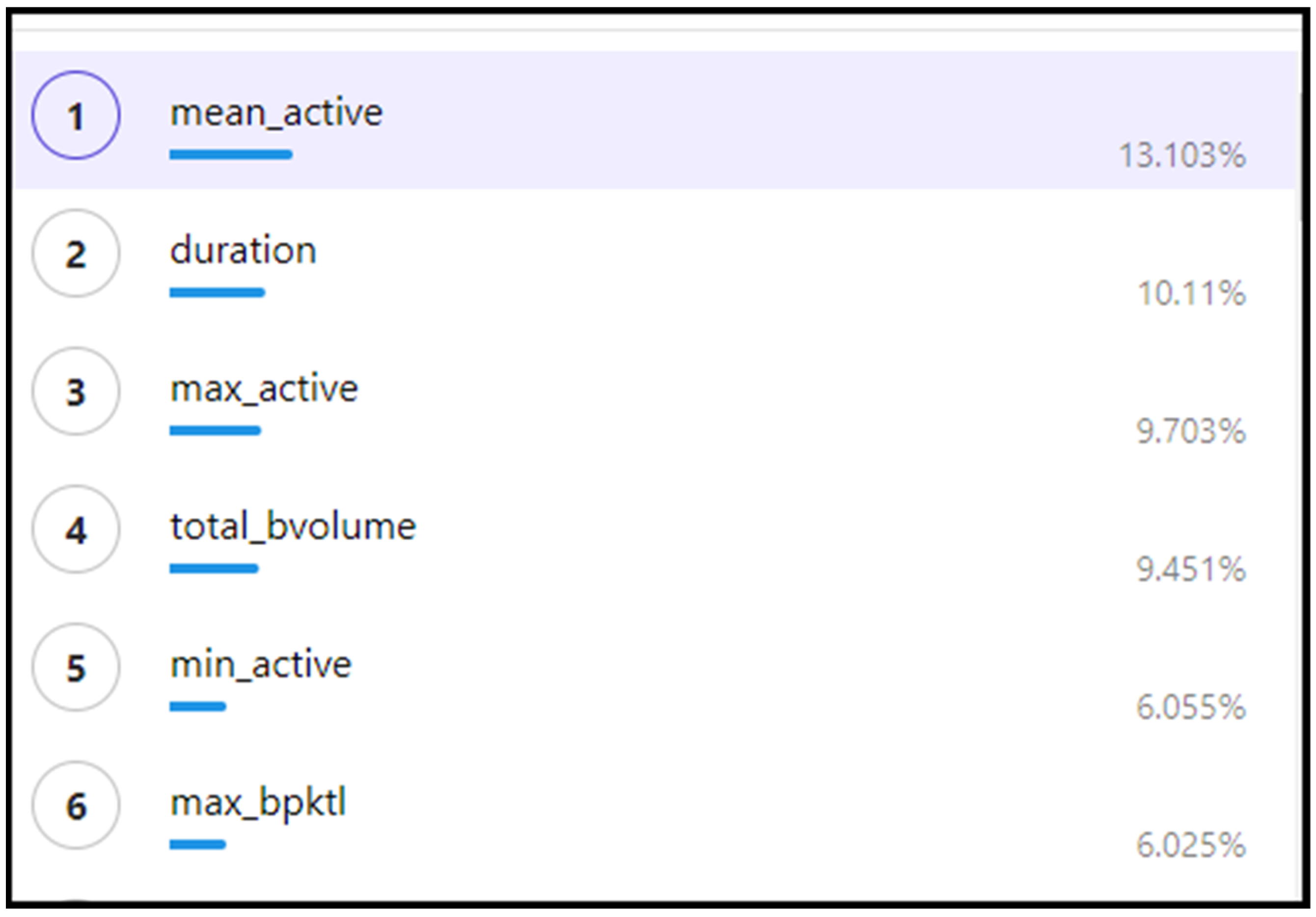
Figure 8. Flow diagram showing the feature redaction process.

5.5. Training and Testing with the Minimum Number of Features with the DL Algorithm

Following the process discussed in Section 5.4, it was determined that the minimum number of features that could be used by the DL algorithm are as follows: total_fvolume, total_bpackets, total_bvolume, min_fpktl, mean_fpktl, max_fpktl, std_fpktl, min_bpktl, mean_bpktl, max_bpktl, std_bpktl, sflow_fbytes, sflow_bbytes, bpsh_cnt, duration, min_active, mean_active, max_active, min_idle and max_idle. The precision, recall and f1-score results can be seen in Table 10 and the confusion matrices can be seen in Table 11.

Table 10. Predication results when using the DL algorithm with minimum features.

Dataset Name	Benign Precision Score	Benign Recall Score	Benign f1-Score	Malware Precision Score	Malware Recall Score	Malware f1-Score
Dataset1	0.98	0.97	0.97	0.97	0.98	0.97
Dataset2	0.9	0.97	0.93	0.97	0.89	0.93
Dataset3	0.9	0.97	0.94	0.97	0.9	0.93
Dataset4	0.66	0.95	0.78	0.92	0.51	0.66
Dataset5	0.67	0.97	0.79	0.95	0.51	0.67
Dataset6	0.79	0.99	0.88	0.98	0.74	0.85
Dataset7	0.97	0.97	0.97	0.97	0.97	0.97
Dataset8	0.91	0.94	0.92	0.94	0.9	0.92
Dataset9	0.92	0.98	0.95	0.98	0.91	0.95

Table 11. Confusion matrix for testing the DL algorithm with minimum features.

Dataset Name	Benign Precision Score	Benign Recall Score	Benign f1-Score	Malware Precision Score	Malware Recall Score	Malware f1-Score
Dataset1	272,425	265,049	7376	272,425	266,052	6373
Dataset2	66,009	64,028	1981	66,009	58,811	7198
Dataset3	38,282	37,298	984	38,282	34,304	3978
Dataset4	200,000	190,820	9180	200,000	102,371	97,629
Dataset5	35,054	34,103	951	35,054	17,996	17,058
Dataset6	6049	5963	86	6049	4499	1550
Dataset7	11,864	11,553	311	11,864	11,535	329
Dataset8	10,204	9575	629	10,204	9233	971
Dataset9	7152	7015	137	7152	6544	608

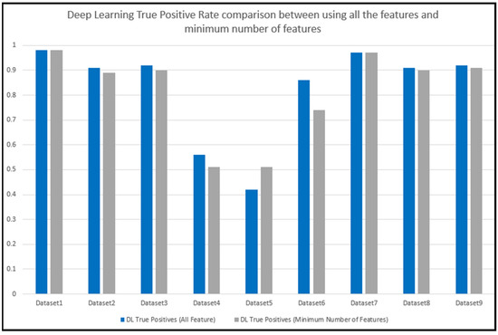
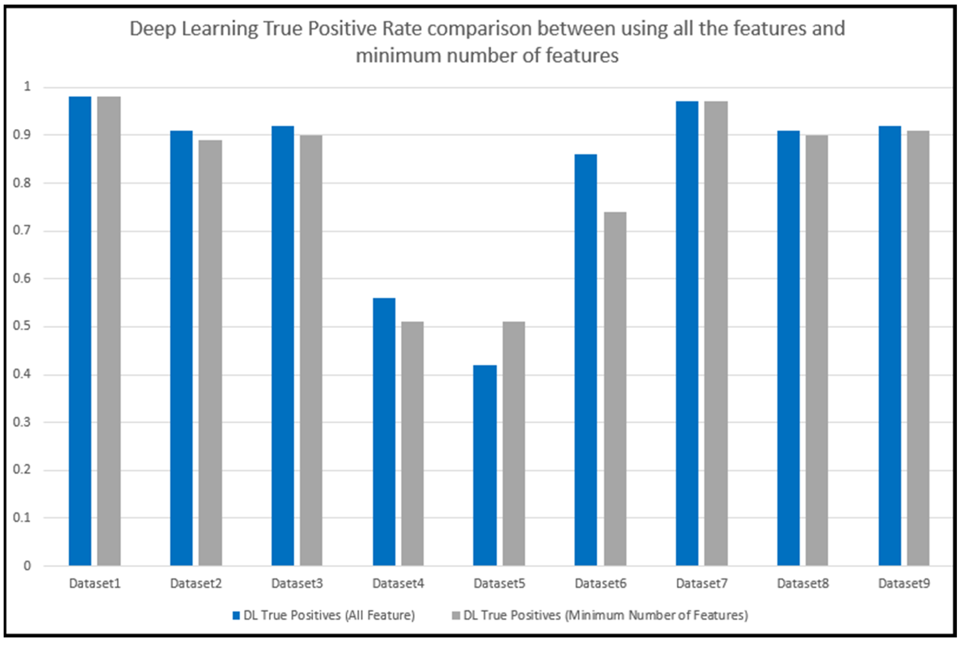
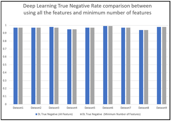
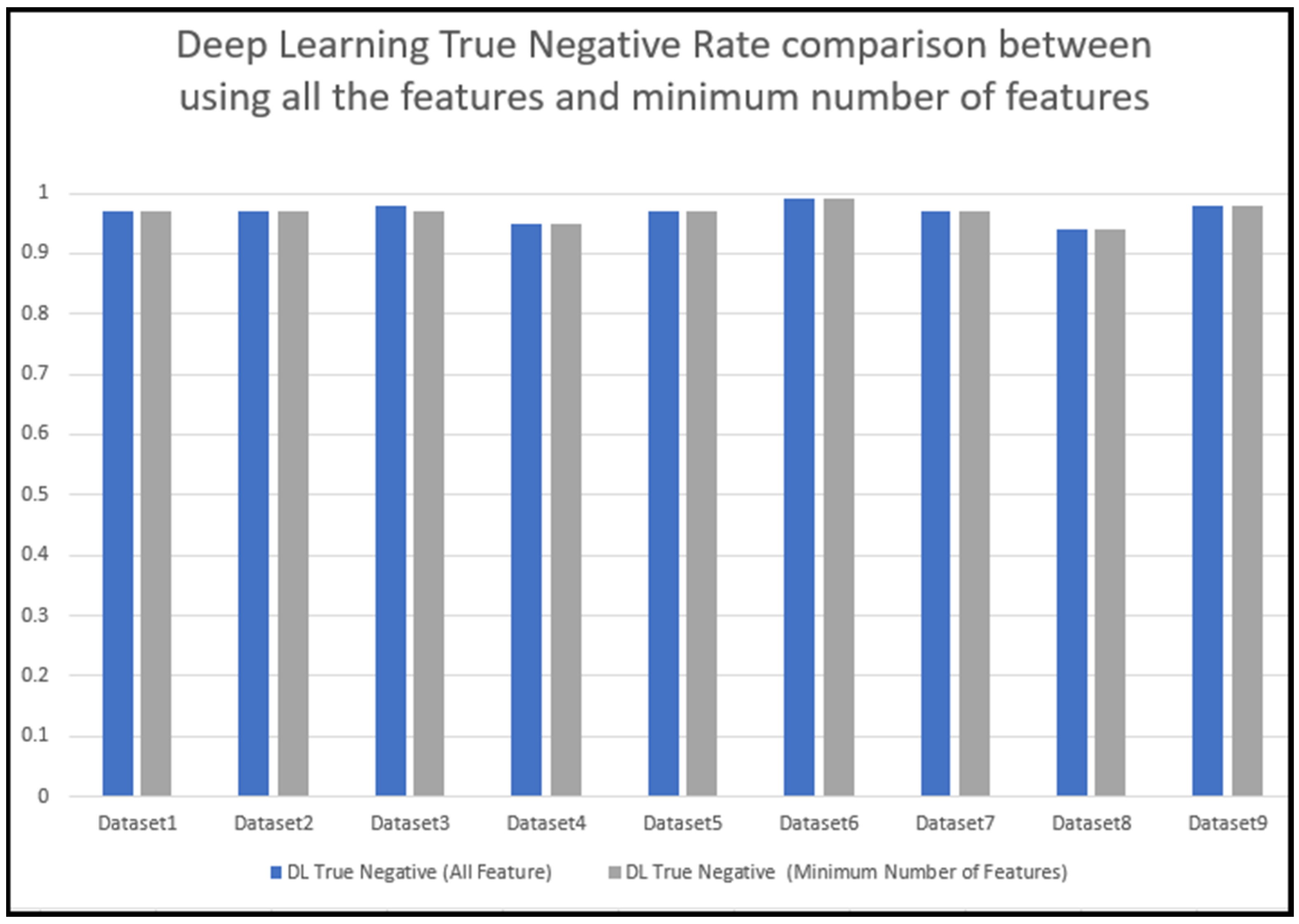
Figure 9 compares the results of detecting the Zeus malware between using all the features and the minimum number of features. The prediction results of dataset1, dataset2, dataset3, dataset4, dataset7, dataset8 and dataset9 were all within 5% of each other, dataset5 was within 9% and dataset6 was within 12%. Figure 10 compares the results of detecting the benign samples between using all the features and the minimum number of features when tested with the deep learning algorithm and shows that the prediction results of all the datasets were within 1% of each other.

Figure 9. Zeus prediction results when tested using the minimum number of features.

Figure 10. Benign communication prediction results when tested using the minimum number of features.

5.6. Training and testing using the minimum number of features with the DT algorithm

Similar experiments were conducted using the DT algorithm and it was determined that the minimum number of features that could be used by the DT algorithm are: total_fvolume, total_bpackets, total_bvolume, min_fpktl, mean_fpktl, max_fpktl, min_bpktl, mean_bpktl, max_bpktl, std_bpktl, sflow_fbytes, sflow_bbytes, furg_cnt, burg_cnt, duration, min_active, mean_active, max_active, min_idle and max_idle.

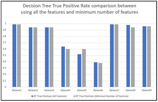
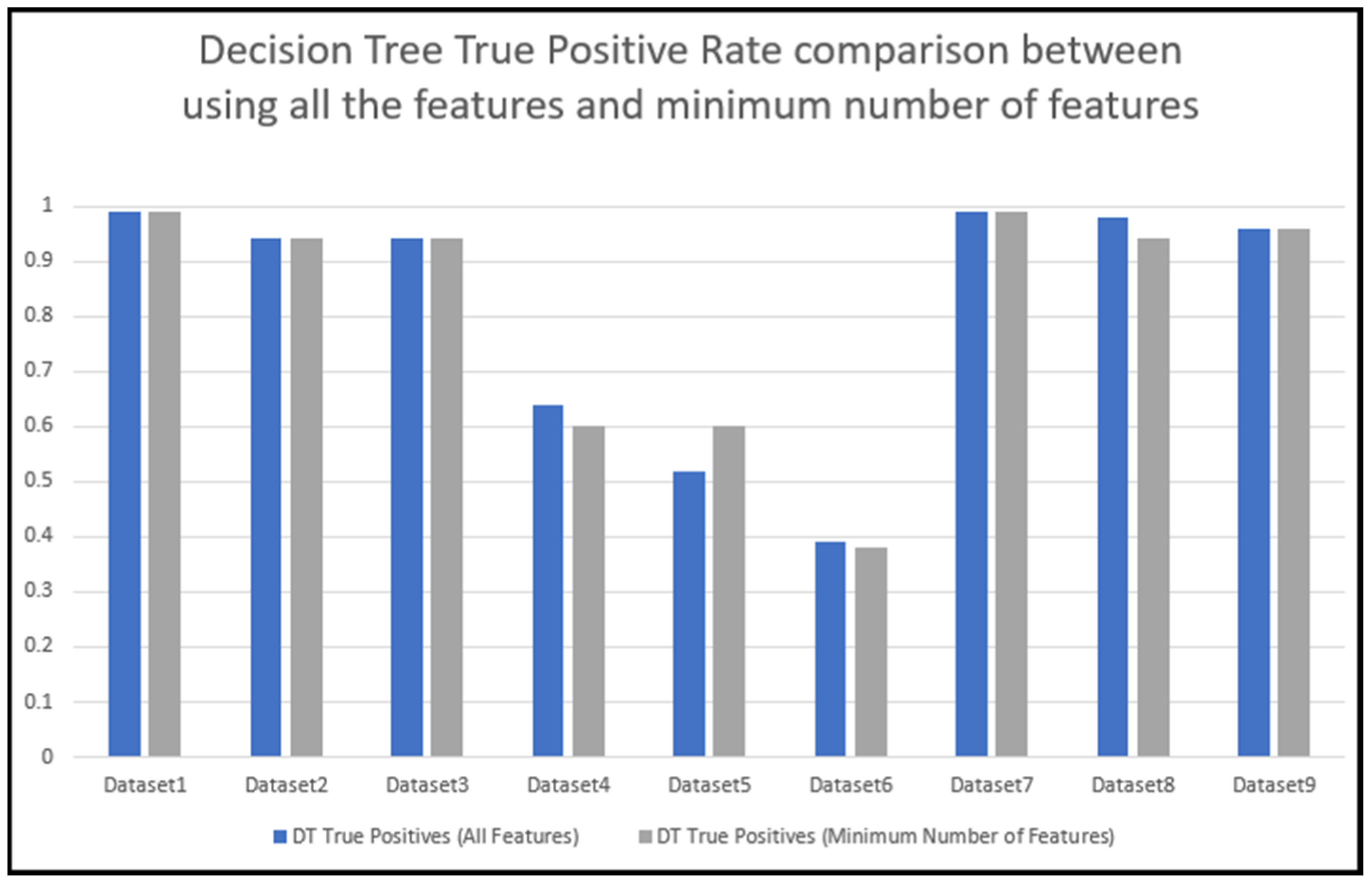
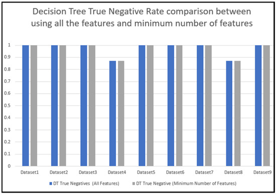
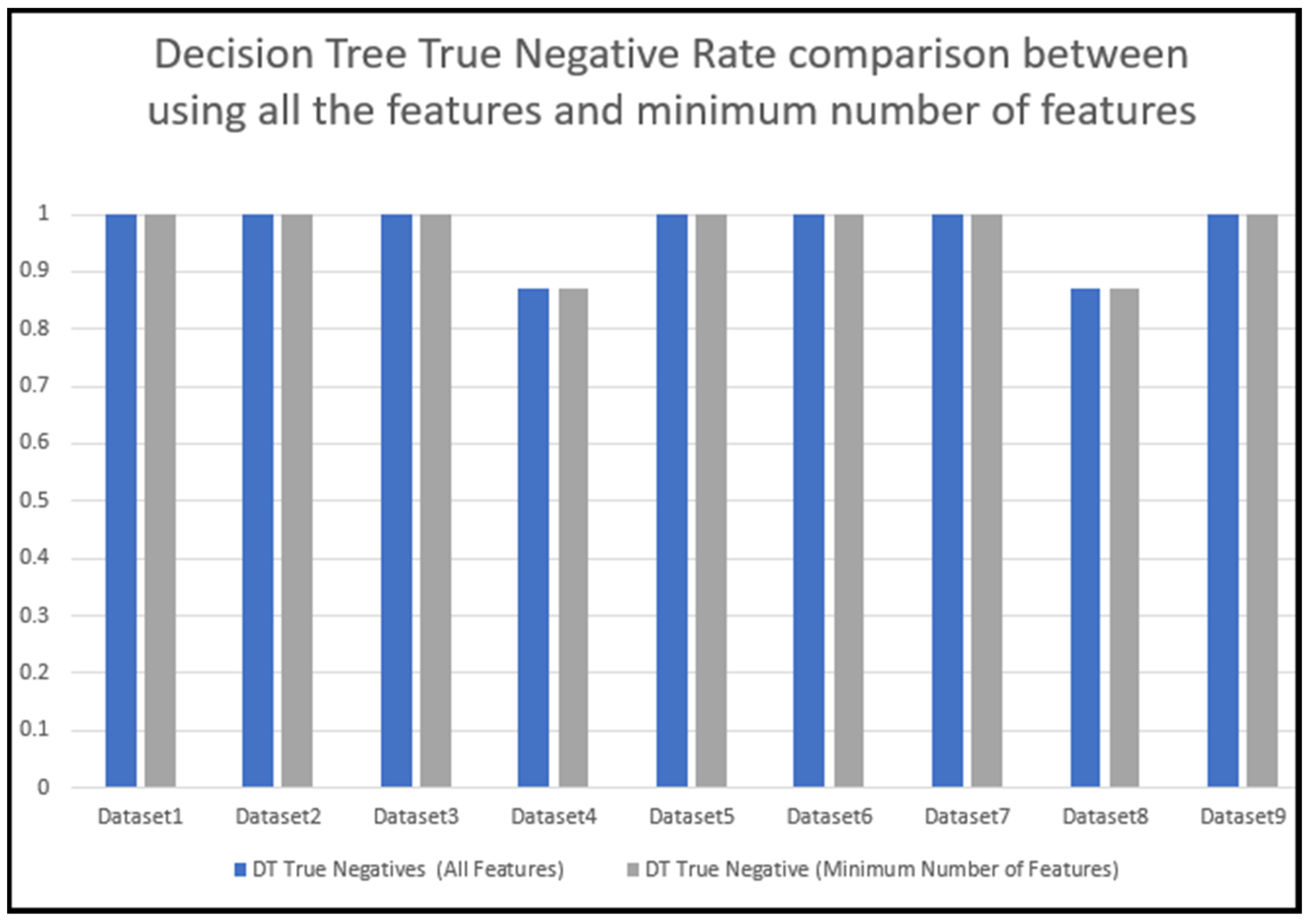
The precision, recall and f1-score results can be seen in Table 12, and the confusion matrices can be seen in Table 13. Figure 11 compares the results of detecting the Zeus malware between using all the features and the minimum number of features and shows that the prediction results of dataset1, dataset2, dataset3, dataset4, dataset6, dataset7, dataset8 and dataset9 were all within 5% of each other, and dataset5 was within 8%. Figure 12 compares the results of detecting the benign samples between using all the features and the minimum number of features and shows that the prediction results of all the datasets are within 1% of each other.

Table 12. Predication results when using the DT algorithm with minimum features.

Dataset Name	Benign Precision Score	Benign Recall Score	Benign f1-Score	Malware Precision Score	Malware Recall Score	Malware f1-Score
Dataset1	0.99	1	0.99	1	0.99	0.99
Dataset2	0.94	1	0.97	1	0.94	0.97
Dataset3	0.94	1	0.97	1	0.94	0.97
Dataset4	0.69	0.87	0.77	0.82	0.6	0.7
Dataset5	0.71	1	0.83	0.99	0.6	0.75
Dataset6	0.62	1	0.76	0.99	0.38	0.55
Dataset7	0.99	1	0.99	1	0.99	0.99
Dataset8	0.94	0.87	0.9	0.88	0.94	0.91
Dataset9	0.96	1	0.98	1	0.96	0.98

Table 13. Confusion matrix for testing the DT algorithm with minimum features.

Dataset Name	Benign Precision Score	Benign Recall Score	Benign f1-Score	Malware Precision Score	Malware Recall Score	Malware f1-Score
Dataset1	272,425	271,502	923	272,425	270,408	2017
Dataset2	66,009	65,788	221	66,009	61,804	4205
Dataset3	38,282	38,159	123	38,282	36,018	2264
Dataset4	200,000	174,267	25,733	200,000	120,785	79,215
Dataset5	35,054	34,935	119	35,054	20,984	14,070
Dataset6	6049	6032	17	6049	2328	3721
Dataset7	11,864	11,825	39	11,864	11,724	140
Dataset8	10,204	8857	1347	10,204	9630	574
Dataset9	7152	7130	22	7152	6837	315

Figure 11. DT Zeus prediction results compared between using the minimum number of features and all the features in Feature set1.

Figure 12. DT benign communication prediction results compared between using the minimum number of features and all the features in Feature set1.

5.7. Training and Testing Using the Minimum Number of Features with the RF Algorithm

Multiple experiments were conducted using the RF algorithm and the features were manually reduced by following the process described above (Section 5.4). This process was repeated until two of the dataset prediction results fell below 50% and it was determined that the minimum number of features that could be used are as follows: total_fvolume, total_bvolume, min_fpktl, mean_fpktl, max_fpktl, min_bpktl, mean_bpktl, max_bpktl, std_bpktl, sflow_fbytes, sflow_bbytes, bpsh_cnt, duration, min_active, mean_active, max_active and min_idle. The precision, recall and f1-score results for testing all the datasets using the minimum number of features with the RF algorithm can be seen in Table 14 and the confusion matrices can be seen in Table 15.

Table 14. Predication results when using the RF algorithm with minimum features.

Dataset Name	Benign Precision Score	Benign Recall Score	Benign f1-Score	Malware Precision Score	Malware Recall Score	Malware f1-Score
Dataset1	1	1	1	1	1	1
Dataset2	0.93	1	0.95	1	0.93	0.95
Dataset3	0.94	1	0.97	1	0.93	0.96
Dataset4	0.67	0.89	0.77	0.84	0.57	0.68
Dataset5	0.7	1	0.83	1	0.58	0.73
Dataset6	0.62	1	0.77	1	0.39	0.56
Dataset7	0.99	1	0.99	1	0.99	0.99
Dataset8	0.99	0.89	0.93	0.9	0.99	0.94
Dataset9	0.96	1	0.98	1	0.96	0.98

Table 15. Confusion matrix for testing the RF algorithm with minimum features.

Dataset Name	Benign Precision Score	Benign Recall Score	Benign f1-Score	Malware Precision Score	Malware Recall Score	Malware f1-Score
Dataset1	272,425	272,233	192	272,425	271,328	1097
Dataset2	66,009	65,961	48	66,009	61,230	4779
Dataset3	38,282	38,256	26	38,282	35,641	2641
Dataset4	200,000	178,346	21,654	200,000	114,030	85,970
Dataset5	35,054	35,029	25	35,054	20,221	14,833
Dataset6	6049	6047	2	6049	2352	3697
Dataset7	11,864	11,855	9	11,864	11,743	121
Dataset8	10,204	9033	1171	10,204	10,081	123
Dataset9	7152	7148	4	7152	6849	303

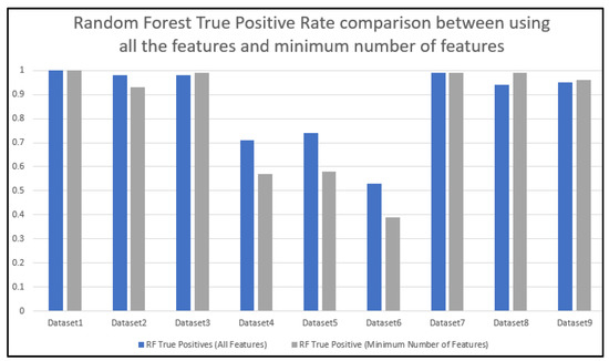
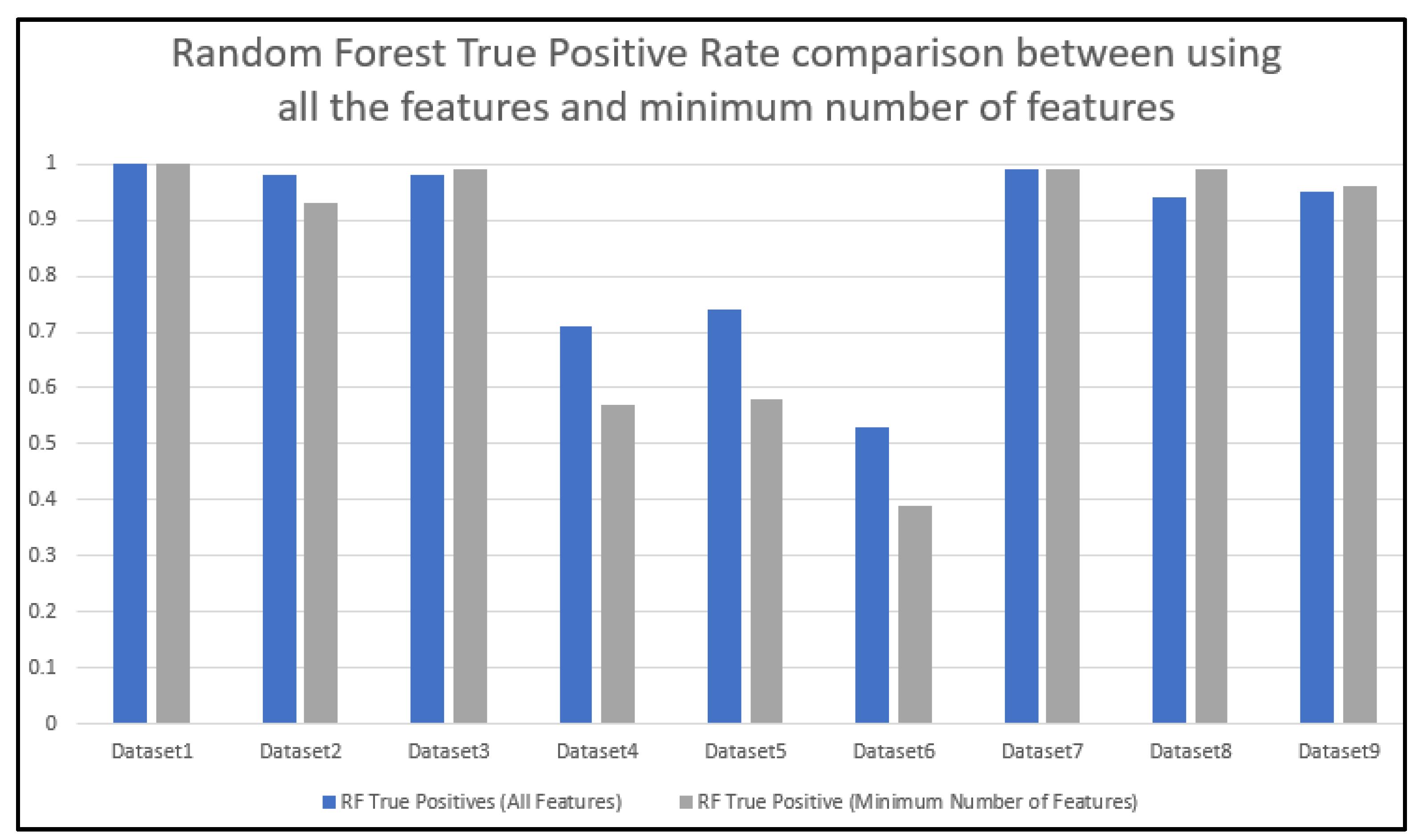
Figure 13 compares the results of detecting the Zeus malware between using all the features and the minimum number of features when tested with the DT algorithm, and shows that the prediction results of dataset1, dataset2, dataset3, dataset7, dataset8 and dataset9 were all within 5% of each other and that dataset4, dataset5 and dataset6 were within 16% of each other. Figure 12 compares the results of detecting the benign samples between using all the features and the minimum number of features and shows that the prediction results of all the datasets were within 1% of each other.

Figure 13. RF Zeus prediction results compared between using the minimum number of features and all the features in Feature set1.

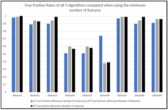
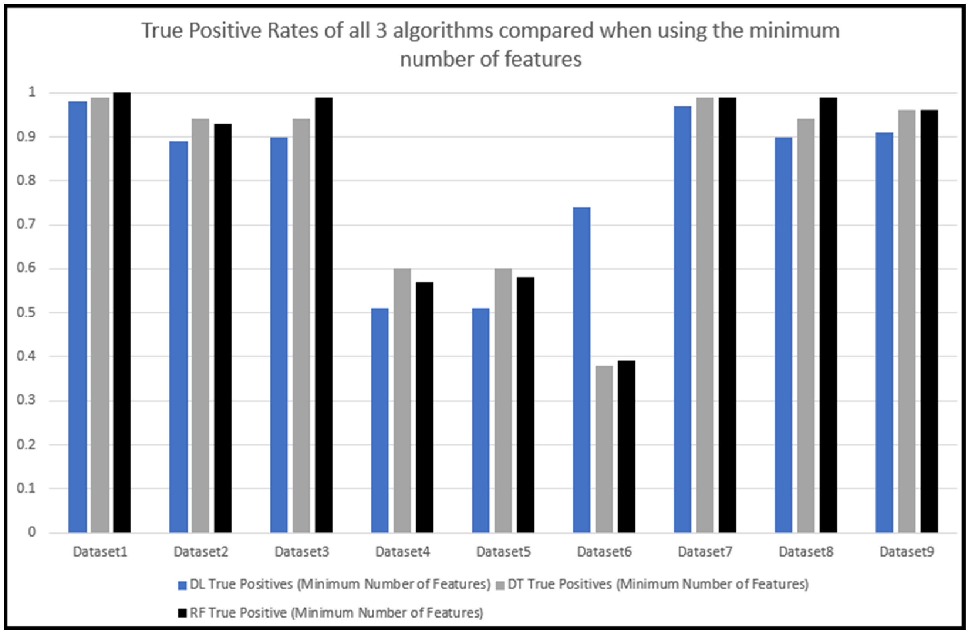
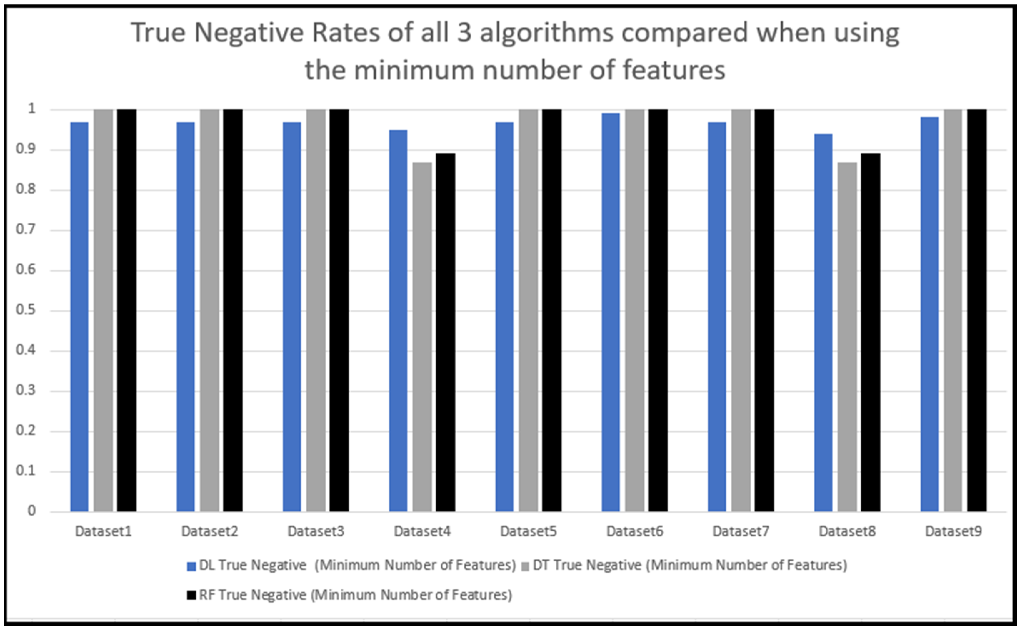
Figure 14 compares the true positive results of all three algorithms when tested using the minimum number of features, and the malware prediction results for all the datasets apart from dataset6 were within 10% of each. Dataset6 was an outlier with a difference of 36%, and in this case, the DL algorithm performing the best with a prediction result of 74% and the DT performing the worst with a prediction result of 38%. Figure 15 compares the results of detecting the benign samples between using all the features and the minimum number of features and shows that the prediction results of all the datasets were within 2% of each other.

Figure 14. True positive rates compared for all three algorithms when using the minimum number of features.

Figure 15. True negative rates compared for all three algorithms when using the minimum number of features.

6. Conclusions

The empirical analysis has shown that the framework and methodology adopted for this research can detect both older and newer versions of the Zeus banking malware, which demonstrates the potential of the framework to detect banking malware that evolve over time. The framework and methodology can also predict other banking malware variants, which demonstrates the potential to detect a wide range of banking malware variants without the need to analyse each banking malware variant to learn about their features.

For future work, there is a potential to further this research by enhancing the methodology to incorporate additional banking malware variants. Moreover, further research can be conducted to detect other malware variants and improve the prediction accuracy when detecting them. Researchers can also further this research by designing and building an IDS solution that could detect a wide range of malware, and the findings from this research could be used for this and by anti-malware vendors when they design malware detection tools. Action on the malicious traffic could also be taken once the malware has been detected. The findings from this research can be used by other researchers to develop their own malware prediction tools to enhance their research.

References

- Wadhwa, A.; Arora, N. A Review on Cyber Crime: Major Threats and Solutions. Int. J. Adv. Res. Comput. Sci. 2017, 8, 2217–2221. [Google Scholar]
- Morgan, S. Cybercrime to Cost the World $10.5 Trillion Annually by 2025. Available online: https://cybersecurityventures.com/hackerpocalypse-cybercrime-report-2016/ (accessed on 2 November 2022).
- Nokia Banking Malware Threats Surging as Mobile Banking Increases–Nokia Threat Intelligence Report. Available online: https://www.nokia.com/about-us/news/releases/2021/11/08/banking-malware-threats-surging-as-mobile-banking-increases-nokia-threat-intelligence-report/ (accessed on 2 November 2022).
- Vijayalakshmi, Y.; Natarajan, N.; Manimegalai, P.; Babu, S.S. Study on emerging trends in malware variants. Int. J. Pure Appl. Math. 2017, 116, 479–489. [Google Scholar]
- Etaher, N.; Weir, G.R.; Alazab, M. From zeus to zitmo: Trends in banking malware. In Proceedings of the 2015 IEEE Trustcom/BigDataSE/ISPA, Helsinki, Finland, 20–22 August 2015; IEEE: Washington, DC, USA, 2015; Volume 1, pp. 1386–1391. [Google Scholar]
- Ibrahim, L.M.; Thanon, K.H. Botnet Detection on the Analysis of Zeus Panda Financial Botnet. Int. J. Eng. Adv. Technol. 2019, 8, 1972–1976. [Google Scholar] [CrossRef] [Scilit]
- Owen, H.; Zarrin, J.; Pour, S.M. A Survey on Botnets, Issues, Threats, Methods, Detection and Prevention. J. Cybersecur. Priv. 2022, 2, 74–88. [Google Scholar] [CrossRef] [Scilit]
- Tayyab, U.-E.; Khan, F.B.; Durad, M.H.; Khan, A.; Lee, Y.S. A Survey of the Recent Trends in Deep Learning Based Malware Detection. J. Cybersecur. Priv. 2022, 2, 800–829. [Google Scholar] [CrossRef] [Scilit]
- Aboaoja, F.A.; Zainal, A.; Ghaleb, F.A.; Al-rimy, B.A.S.; Eisa, T.A.E.; Elnour, A.A.H. Malware Detection Issues, Challenges, and Future Directions: A Survey. Appl. Sci. 2022, 12, 8482. [Google Scholar] [CrossRef] [Scilit]
- Ahsan, M.; Nygard, K.E.; Gomes, R.; Chowdhury, M.M.; Rifat, N.; Connolly, J.F. Cybersecurity Threats and Their Mitigation Approaches Using Machine Learning—A Review. J. Cybersecur. Priv. 2022, 2, 527–555. [Google Scholar] [CrossRef] [Scilit]
- Bukvić, L.; Pašagić Škrinjar, J.; Fratrović, T.; Abramović, B. Price Prediction and Classification of Used-Vehicles Using Supervised Machine Learning. Sustainability 2022, 14, 17034. [Google Scholar] [CrossRef] [Scilit]
- Okey, O.D.; Maidin, S.S.; Adasme, P.; Lopes Rosa, R.; Saadi, M.; Carrillo Melgarejo, D.; Zegarra Rodríguez, D. BoostedEnML: Efficient Technique for Detecting Cyberattacks in IoT Systems Using Boosted Ensemble Machine Learning. Sensors 2022, 22, 7409. [Google Scholar] [CrossRef] [Scilit]
- Singh, A.; Thakur, N.; Sharma, A. A review of supervised machine learning algorithms. In Proceedings of the 2016 3rd International Conference on Computing for Sustainable Global Development 2016, (INDIACom), New Delhi, India, 16–18 March 2016; pp. 1310–1315. [Google Scholar]
- Aswathi, K.B.; Jayadev, S.; Krishna, N.; Krishnan, R.; Sarath, G. Botnet Detection using Machine Learning. In Proceedings of the 2021 12th International Conference on Computing Communication and Networking Technologies (ICCCNT), Kharagpur, India, 6–8 July 2021; pp. 1–7. [Google Scholar] [CrossRef] [Scilit]
- Kazi, M.; Woodhead, S.; Gan, D. A contempory Taxonomy of Banking Malware. In Proceedings of the First International Conference on Secure Cyber Computing and Communications, Jalandhar, India, 15–17 December 2018. [Google Scholar]
- Falliere, N.; Chien, E. Zeus: King of the Bots. 2009. Available online: http://bit.ly/3VyFV1 (accessed on 12 November 2022).
- Lelli, A. Zeusbot/Spyeye P2P Updated, Fortifying the Botnet. Available online: https://www.symantec.com/connect/blogs/zeusbotspyeye-p2p-updated-fortifying-botnet (accessed on 5 November 2019).
- Riccardi, M.; Di Pietro, R.; Palanques, M.; Vila, J.A. Titans’ Revenge: Detecting Zeus via Its Own Flaws. Comput. Netw. 2013, 57, 422–435. [Google Scholar] [CrossRef] [Scilit]
- Andriesse, D.; Rossow, C.; Stone-Gross, B.; Plohmann, D.; Bos, H. Highly Resilient Peer-to-Peer Botnets Are Here: An Analysis of Gameover Zeus. In Proceedings of the 2013 8th International Conference on Malicious and Unwanted Software: “The Americas” (MALWARE), Fajardo, PR, USA, 22–24 October 2013; pp. 116–123. [Google Scholar]
- Kazi, M.A.; Woodhead, S.; Gan, D. Comparing the performance of supervised machine learning algorithms when used with a manual feature selection process to detect Zeus malware. Int. J. Grid Util. Comput. 2022, 13, 495–504. [Google Scholar] [CrossRef] [Scilit]
- Md, A.Q.; Jaiswal, D.; Daftari, J.; Haneef, S.; Iwendi, C.; Jain, S.K. Efficient Dynamic Phishing Safeguard System Using Neural Boost Phishing Protection. Electronics 2022, 11, 3133. [Google Scholar] [CrossRef] [Scilit]
- Ibrahim, L.M.; Thanon, K.H. Analysis and detection of the zeus botnet crimeware. Int. J. Comput. Sci. Inf. Secur. 2015, 13, 121. [Google Scholar]
- Gu, G.; Porras, P.; Yegneswaran, V.; Fong, M.; Lee, W. BotHunter: Detecting Malware Infection Through IDS-Driven Dialog Correlation. In Proceedings of the USENIX Conference on Security Symposium, Anaheim, CA, USA, 9–11 August 2007; pp. 167–182. [Google Scholar]
- Thorat, S.A.; Khandelwal, A.K.; Bruhadeshwar, B.; Kishore, K. Payload Content Based Network Anomaly Detection. In Proceedings of the 2008 First International Conference on the Applications of Digital Information and Web Technologies (ICADIWT), Ostrava, Czech Republic, 4–6 August 2008. [Google Scholar] [CrossRef] [Scilit]
- Guofei, G.; Perdisci, R.; Zhang, J.; Lee, W. BotMiner: Clustering analysis of network traffic for protocol- and structure-independent botnet detection. In Proceedings of the 17th Conference on Security Symposium, San Jose, CA, USA, 28 July–1 August 2008; pp. 139–154. [Google Scholar]
- Azab, A.; Alazab, M.; Aiash, M. Machine Learning Based Botnet Identification Traffic. In Proceedings of the 2016 IEEE Trustcom/BigDataSE/ISPA, Tianjin, China, 23–26 August 2016; pp. 1788–1794. [Google Scholar]
- Soniya, B.; Wilscy, M. Detection of Randomized Bot Command and Control Traffic on an End-Point Host. Alex. Eng. J. 2016, 55, 2771–2781. [Google Scholar] [CrossRef] [Scilit]
- Venkatesh, G.K.; Nadarajan, R.A. HTTP botnet detection using adaptive learning rate multilayer feed-forward neural network. In Proceedings of the IFIP International Workshop on Information Security Theory and Practice, Egham, UK, 20–22 June 2012; Springer: Berlin/Heidelberg, Germany, 2012; Volume 7322 LNCS, pp. 38–48. [Google Scholar]
- Haddadi, F.; Runkel, D.; Zincir-Heywood, A.N.; Heywood, M.I. On Botnet Behaviour Analysis Using GP and C4.5; Association for Computing Machinery: New York, NY, USA, 2014; pp. 1253–1260. [Google Scholar]
- Fernandez, D.; Lorenzo, H.; Novoa, F.J.; Cacheda, F.; Carneiro, V. Tools for managing network traffic flows: A comparative analysis. In Proceedings of the 2017 IEEE 16th International Symposium on Network Computing and Applications (NCA), Cambridge, MA, USA, 30 October–1 November 2017; IEEE: Piscataway, NJ, USA, 2017; pp. 1–5. [Google Scholar]
- Fuhr, J.; Wang, F.; Tang, Y. MOCA: A Network Intrusion Monitoring and Classification System. J. Cybersecur. Priv. 2022, 2, 629–639. [Google Scholar] [CrossRef] [Scilit]
- He, S.; Zhu, J.; He, P.; Lyu, M.R. Experience report: System log analysis for anomaly detection. In Proceedings of the 2016 IEEE 27th international symposium on software reliability engineering (ISSRE), Ottawa, ON, Canada, 23–27 October 2016; pp. 207–218. [Google Scholar]
- Zhou, J.; Qian, Y.; Zou, Q.; Liu, P.; Xiang, J. DeepSyslog: Deep Anomaly Detection on Syslog Using Sentence Embedding and Metadata. IEEE Trans. Inf. Forensics Secur. 2022, 17, 3051–3061. [Google Scholar] [CrossRef] [Scilit]
- Ghafir, I.; Prenosil, V.; Hammoudeh, M.; Baker, T.; Jabbar, S.; Khalid, S.; Jaf, S. BotDet: A System for Real Time Botnet Command and Control Traffic Detection. IEEE Access 2018, 6, 38947–38958. [Google Scholar] [CrossRef] [Scilit]
- Agarwal, P.; Satapathy, S. Implementation of signature-based detection system using snort in windows. Int. J. Comput. Appl. Inf. Technol. 2014, 3, 3–4. [Google Scholar]
- Khraisat, A.; Gondal, I.; Vamplew, P.; Kamruzzaman, J. Survey of intrusion detection systems: Techniques, datasets and challenges. Cybersecurity 2019, 2, 1–22. [Google Scholar] [CrossRef] [Scilit]
- Sharma, P.; Said, Z.; Memon, S.; Elavarasan, R.M.; Khalid, M.; Nguyen, X.P.; Arıcı, M.; Hoang, A.T.; Nguyen, L.H. Comparative evaluation of AI-based intelligent GEP and ANFIS models in prediction of thermophysical properties of Fe3O4-coated MWCNT hybrid nanofluids for potential application in energy systems. Int. J. Energy Res. 2022, 37, 19242–19257. [Google Scholar] [CrossRef] [Scilit]
- Arndt, D. DanielArndt/Netmate-Flowcalc. Available online: https://github.com/DanielArndt/netmate-flowcalc (accessed on 6 November 2019).
- Montigny-Leboeuf, A.D.; Couture, M.; Massicotte, F. Traffic Behaviour Characterization Using NetMate. In International Workshop on Recent Advances in Intrusion Detection 2019; Springer: Berlin/Heidelberg, Germany; pp. 367–368.
- De Montigny-Leboeuf, A.; Couture, M.; Massicotte, F. Traffic Behaviour Characterization Using NetMate. Lect. Notes Comput. Sci. 2009, 5758, 367–368. [Google Scholar] [CrossRef] [Scilit]
- de Menezes, N.A.T.; de Mello, F.L. Flow Feature-Based Network Traffic Classification Using Machine Learning. J. Inf. Secur. Cryptogr. 2021, 8, 12–16. [Google Scholar] [CrossRef] [Scilit]
- Miller, S.; Curran, K.; Lunney, T. Multilayer perceptron neural network for detection of encrypted VPN network traffic. In Proceedings of the International Conference On Cyber Situational Awareness, Data Analytics And Assessment (Cyber SA), Glasgow, UK, 11–12 June 2018. [Google Scholar]
- Kasongo, S.M.; Sun, Y. A Deep Learning Method with Filter Based Feature Engineering for Wireless Intrusion Detection System. IEEE Access 2019, 7, 38597–38607. [Google Scholar] [CrossRef] [Scilit]
- Reis, B.; Maia, E.; Praça, I. Selection and Performance Analysis of CICIDS2017 Features Importance. Found. Pract. Secur. 2020, 12056, 56–71. [Google Scholar] [CrossRef] [Scilit]
- Maldonado, S.; Weber, R. A wrapper method for feature selection using Support Vector Machines. Inf. Sci. 2009, 179, 2208–2217. [Google Scholar] [CrossRef] [Scilit]
- Wald, R.; Khoshgoftaar, T.; Napolitano, A. Comparison of Stability for Different Families of Filter-Based and Wrapper-Based Feature Selection. In Proceedings of the 2013 12th International Conference on Machine Learning and Applications, Miami, FL, USA, 4–7 December 2013. [Google Scholar] [CrossRef] [Scilit]
- Schmoll, C.; Zander, S. NetMate-User and Developer Manual. 2004. Available online: https://www.researchgate.net/publication/246926554_NetMate-User_and_Developer_Manual (accessed on 22 December 2022).
- Saghezchi, F.B.; Mantas, G.; Violas, M.A.; de Oliveira Duarte, A.M.; Rodriguez, J. Machine Learning for DDoS Attack Detection in Industry 4.0 CPPSs. Electronics 2022, 11, 602. [Google Scholar] [CrossRef] [Scilit]
- Alshammari, R.; Zincir-Heywood, A.N. Investigating Two Different Approaches for Encrypted Traffic Classification. In Proceedings of the 2008 Sixth Annual Conference on Privacy, Security and Trust, Fredericton, NB, Canada, 1–3 October 2008. [Google Scholar] [CrossRef] [Scilit]
- Yeo, M.; Koo, Y.; Yoon, Y.; Hwang, T.; Ryu, J.; Song, J.; Park, C. Flow-Based Malware Detection Using Convolutional Neural Network. In Proceedings of the 2018 International Conference on Information Networking (ICOIN), Chiang Mai, Thailand, 10–12 January 2018. [Google Scholar] [CrossRef] [Scilit]
- Shomiron. Zeustracker. Available online: https://github.com/dnif-archive/enrich-zeustracker (accessed on 25 July 2022).
- Stratosphere. Stratosphere Laboratory Datasets. Available online: https://www.stratosphereips.org/datasets-overview (accessed on 25 November 2022).
- Abuse, C. Fighting Malware and Botnets. Available online: https://abuse.ch/ (accessed on 13 May 2022).
- Haddadi, F.; Zincir-Heywood, A.N. Benchmarking the effect of flow exporters and protocol filters on botnet traffic classification. IEEE Syst. J. 2014, 10, 1390–1401. [Google Scholar] [CrossRef] [Scilit]
- Khodamoradi, P.; Fazlali, M.; Mardukhi, F.; Nosrati, M. Heuristic metamorphic malware detection based on statistics of assembly instructions using classification algorithms. In Proceedings of the 2015 18th CSI International Symposium on Computer Architecture and Digital Systems (CADS), Tehran, Iran, 7–8 October 2015; pp. 1–6. [Google Scholar]
- Salzberg, S.L. C4.5: Programs for Machine Learning by J. Ross Quinlan; Morgan Kaufmann Publishers, Inc.: Burlington, MA, USA, 1993. [Google Scholar]
- Xhemali, D.; Hinde, C.J.; Stone, R.G. Naïve Bayes vs. Decision Trees vs. Neural Networks in the Classification of Training Web Pages. Int. J. Comput. Sci. Issues 2009, 4, 16–23. [Google Scholar]
- Bernard, S.; Heutte, L.; Adam, S. On the selection of decision trees in random forests. In Proceedings of the 2009 International Joint Conference on Neural Networks, Atlanta, GA, USA, 14–19 June 2009; pp. 302–307. [Google Scholar]
- Maimon, O.; Rokach, L. (Eds.) Data Mining and Knowledge Discovery Handbook; Springer: Berlin/Heidelberg, Germany, 2005. [Google Scholar]
- Liu, Z.; Thapa, N.; Shaver, A.; Roy, K.; Siddula, M.; Yuan, X.; Yu, A. Using Embedded Feature Selection and CNN for Classification on CCD-INID-V1—A New IoT Dataset. Sensors 2021, 21, 4834. [Google Scholar] [CrossRef] [Scilit]
- Oshiro, T.M.; Perez, P.S.; Baranauskas, J.A. How Many Trees in a Random Forest? Mach. Learn. Data Min. Pattern Recognit. 2012, 7376, 154–168. [Google Scholar] [CrossRef] [Scilit]
- Jiang, Z.; Shen, G. Prediction of House Price Based on the Back Propagation Neural Network in the Keras Deep Learning Framework. In Proceedings of the 2019 6th International Conference on Systems and Informatics (ICSAI), Shanghai, China, 2–4 November 2019; pp. 1408–1412. [Google Scholar] [CrossRef] [Scilit]
- Nagisetty, A.; Gupta, G.P. Framework for detection of malicious activities in IoT networks using keras deep learning library. In Proceedings of the 2019 3rd International Conference on Computing Methodologies and Communication (ICCMC), Erode, India, 27–29 March 2019; pp. 633–637. [Google Scholar]
- Heller, M. What Is Keras? The Deep Neural Network API Explained. Available online: https://www.infoworld.com/article/3336192/what-is-keras-the-deep-neural-network-api-explained.html (accessed on 25 November 2022).
- Ali, S.; Rehman, S.U.; Imran, A.; Adeem, G.; Iqbal, Z.; Kim, K.-I. Comparative Evaluation of AI-Based Techniques for Zero-Day Attacks Detection. Electronics 2022, 11, 3934. [Google Scholar] [CrossRef] [Scilit]
- Kumar, V.; Lalotra, G.S.; Sasikala, P.; Rajput, D.S.; Kaluri, R.; Lakshmanna, K.; Shorfuzzaman, M.; Alsufyani, A.; Uddin, M. Addressing Binary Classification over Class Imbalanced Clinical Datasets Using Computationally Intelligent Techniques. Healthcare 2022, 10, 1293. [Google Scholar] [CrossRef] [Scilit] [PubMed]
- Maudoux, C.; Boumerdassi, S.; Barcello, A.; Renault, E. Combined Forest: A New Supervised Approach for a Machine-Learning-Based Botnets Detection. In Proceedings of the 2021 IEEE Global Communications Conference (GLOBECOM), Madrid, Spain, 7–11 December 2021. [Google Scholar] [CrossRef] [Scilit]
Disclaimer/Publisher’s Note: The statements, opinions and data contained in all publications are solely those of the individual author(s) and contributor(s) and not of MDPI and/or the editor(s). MDPI and/or the editor(s) disclaim responsibility for any injury to people or property resulting from any ideas, methods, instructions or products referred to in the content. |
© 2022 by the authors. Licensee MDPI, Basel, Switzerland. This article is an open access article distributed under the terms and conditions of the Creative Commons Attribution (CC BY) license (https://creativecommons.org/licenses/by/4.0/).