


Abstract
Security Operations Centers increasingly use artificial intelligence to rank alerts, summarize evidence, and automate repetitive response actions. However, AI-enabled security operations can also create new risks for incident response and digital forensic reliability, including false-negative prioritization, model drift, hallucinated explanations, prompt injection, automation bias, unsafe SOAR actions, and evidence contamination. This article proposes a risk-driven deployment and forensic readiness framework for AI-enabled Security Operations Centers. The framework combines Monte Carlo loss simulation, detector threshold analysis, analyst queueing, model-drift monitoring, and evidence-preserving governance controls. It explicitly separates evidence, recommendation, and action so that AI can accelerate triage while preserving source artifacts, provenance, audit trails, and chain-of-custody information needed for incident reconstruction. Illustrative simulation results show a mean annualized loss expectancy of USD 1.70 M, a 95% Value-at-Risk of USD 3.85 M and a 99% Value-at-Risk of USD 6.29 M, a detector ROC-AUC of 0.942 and PR-AUC of 0.750 with precision 0.719, recall 0.650 and F1 0.683 at the selected decision threshold of 1.873, a manual triage workload reduction of about 38%, and a reduction in mean time to respond (MTTR, defined throughout as mean time to respond rather than mean time to resolution) from about 44 to 26 min under controlled assumptions. The results are demonstration outputs rather than universal benchmarks. The main contribution is a reproducible governance method for deciding when AI reduces SOC risk, when it transfers risk, and when forensic readiness requires human approval, evidence preservation, or automation rollback.
1. Introduction
Security Operations Centers (SOCs) are expected to detect, investigate, and respond to cyber incidents in real time. Modern organizations collect telemetry from cloud services, endpoint detection and response systems, identity providers, network sensors, vulnerability scanners, firewalls, threat intelligence feeds, and user-reported events. This visibility is valuable, but it creates a persistent operational problem: analysts must process large alert volumes while still identifying rare but high-impact incidents. Alert fatigue is therefore both a technical and a human risk, because repeated low-value alerts can reduce attention, delay escalation, and weaken trust in the detection process [1].
Incident response guidance emphasizes preparation, detection, analysis, containment, eradication, recovery, and continuous improvement [2]. In practice, SOC actions are also the first stage of later digital forensic work. Alerts, logs, endpoint records, authentication events, cloud activity, and analyst decisions may become the evidence base for incident reconstruction, insurance review, regulatory reporting, internal audit, or legal investigation. For this reason, AI-enabled SOC deployment should be evaluated not only by faster triage and workload reduction, but also by whether it preserves the evidentiary reliability of the incident record.
Digital forensic guidance has long emphasized the need to identify, collect, preserve, and analyze digital evidence in a repeatable and defensible manner [3,4]. Digital evidence is fragile because it can be overwritten, transformed, reinterpreted, or removed during response actions. Classical digital forensic research also shows that investigation quality depends on provenance, temporal ordering, reconstruction logic, and the ability to justify conclusions from source artifacts rather than from unsupported interpretation [5,6]. These requirements become more complex when AI systems are inserted into SOC workflows.
AI is often presented as a solution to alert fatigue. Machine learning models can rank alerts, large language models can summarize evidence, and security orchestration, automation, and response (SOAR) platforms can execute repeatable playbooks. Yet a SOC does not become safer merely because AI is added. A classifier can reduce Tier-1 workload but introduce false negatives. A generative assistant can accelerate reporting but produce unsupported explanations. A playbook can contain a host quickly but also interrupt critical service or modify evidence before collection. AI in the SOC must therefore be evaluated as a risk-control and forensic readiness system, not only as a technical innovation.
This article addresses the following research questions. RQ1: How can AI-enabled SOC deployment be evaluated as a risk-control problem rather than only as an automation problem? RQ2: How can detector performance, analyst workload, model drift, annualized loss, and forensic readiness be connected in one practical evaluation framework? RQ3: Which governance controls are required to ensure that AI-supported triage, LLM assistance, and SOAR automation reduce risk without weakening evidence provenance or incident reconstruction?
The contributions of the paper are threefold. First, it defines a risk and forensic readiness taxonomy for AI-enabled SOCs that include classical cyber risks, detection capability gaps, AI-specific failure modes, and evidence-handling risks. Second, it presents a practical deployment framework that starts with shadow-mode evaluation and only later introduces assisted triage and controlled automation. Third, it provides a reproducible evaluation structure that can be calibrated with local SOC data and accompanied by evidence preservation, provenance logging, human approval gates, and automation stop conditions.
2. Related Work
Research on AI-enabled SOCs connects several studies. The first concerns machine learning for cybersecurity. Machine learning systems can support detection, anomaly scoring, and alert prioritization, but their performance depends on representative training data, stable features, and careful validation [7]. AI-assisted SIEM work shows that machine learning can reduce alert fatigue by ranking likely true positives and attaching context [8]. Alert-prioritization studies similarly show that models can support escalation decisions from historical incident patterns [9]. However, model metrics alone do not explain whether the SOC reduces annualized loss, controls queueing delay, or preserves forensic evidence.
The second stream concerns cyber threat intelligence and contextual enrichment. CTI connects internal observations with external indicators, adversary tactics, malware families, and campaign context [10]. The value of a local alert changes when it maps to a known technique, active campaign, high-value asset, or exploitable vulnerability. ATT&CK can support mapping to adversary behavior [11], while CVSS can help represent vulnerability severity when alerts relate to known weaknesses [12]. In the proposed framework, CTI and asset criticality are not late-stage investigation aids only; they modify priority, loss exposure, and evidence collection.
The third stream concerns SOAR and automated response. SOAR can reduce repetitive enrichment work, enforce standard procedures, and improve response speed [13]. Formal evaluation methods have also been proposed for SOAR tools and limited survey data [14]. Recent work on robust and agentic SOAR emphasizes the need for policy, confidence thresholds, and audit trails [15]. The forensic problem is that automation can change evidence before it is preserved. A risk-driven SOC must therefore distinguish reversible enrichment actions from irreversible containment actions and record who or what triggered each step.
The fourth stream concerns LLMs and security agents. Surveys describe LLM use in SOCs for log summarization, alert explanation, query generation, incident reporting, and analyst assistance [16,17]. Empirical work on human–AI collaboration suggests that analysts benefit most when LLMs support sense-making and communication rather than replacing decision-making [18]. End-to-end LLM frameworks for SOC support are emerging [19]. These developments are promising, but they also require evidence grounding, prompt-injection defenses, provenance checking, and clear separation between source artifacts and generated summaries.
The fifth stream concerns adversarial and governance risks of AI. Machine learning systems can be affected by evasion, poisoning, privacy leakage, and other security failures [20]. The malicious use of AI can also increase attacker capability and speed [21]. LLM-specific guidance further highlights risks such as prompt injection, insecure tool use, sensitive information disclosure, and overreliance [22]. For SOC and forensic use, these risks are operationally significant because they can alter priority scores, contaminate analyst conclusions, or create false confidence in an AI-generated incident narrative.
The sixth stream concerns risk management, digital forensics, and forensic readiness. The NIST AI Risk Management Framework provides a governance vocabulary for mapping, measuring, and managing AI risk [23], while ISO/IEC 27005 supports information-security risk management [24]. FAIR connects cyber decisions to loss and uncertainty [25]. Digital investigation standards and guidance address the assurance of investigation methods [26], incident investigation principles [27], log management [28], and continuous monitoring [29]. Event-based and objectives-based forensic models further emphasize reconstruction, hypothesis testing, and traceable investigation goals [30,31]. Research on data-volume growth, cloud forensics, and investigation challenges shows that modern evidence handling requires scalable and well-governed processes [32,33,34]. This paper integrates these streams by treating AI-SOC deployment as both a risk-control problem and a forensic readiness problem.
Taken together, these six streams supply the components of an AI-enabled SOC but not the decision linkage between them. AI-SIEM and alert-prioritization work optimizes detector metrics without mapping them to residual loss or queue stability; SOAR research optimizes response speed without treating evidence preservation as a precondition for action; AI-risk-management frameworks supply governance vocabulary without operational thresholds; and forensic readiness standards specify evidence obligations without connecting them to model performance. The contribution of this paper is precisely that linkage: a single deployment decision that is conditioned jointly on expected and tail loss, the detector operating threshold, analyst queue stability, the staged automation level, and evidence provenance, so that digital forensics and incident response (DFIR) obligations constrain automation scope rather than being reconciled with it after the fact.
A caveat on the evidence base is appropriate. Several sources cited in the AI-SOC automation and LLM-support discussion [9,14,16,18,19] are arXiv preprints that have not completed peer review. They are cited here because they represent the most current description of a fast-moving practice area, but claims drawn from them are treated as indicative rather than established, and none of the quantitative choices in Section 3 rests on them.
Table 1 summarizes how the six research streams reviewed above contribute to AI-enabled SOC deployment and identifies the remaining gaps that motivate the proposed risk-driven and forensic-readiness framework.
Table 1.
Position of this work in relation to previous cybersecurity, AI-SOC, and digital-forensics research.
3. Materials and Methods
3.1. Design Principles
The proposed method treats the AI-enabled SOC as a controlled socio-technical system whose purpose is to reduce residual cyber risk while maintaining analyst accountability and forensic readiness. The framework is based on four design principles. First, AI may automate evidence collection earlier than it automates decisions. Second, reversible actions may be automated earlier than irreversible actions. Third, generated explanations must be grounded in source artifacts. Fourth, every transition from evidence to recommendation to action must be logged for audit and incident reconstruction.
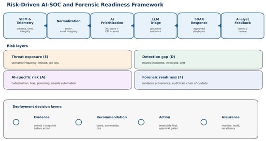
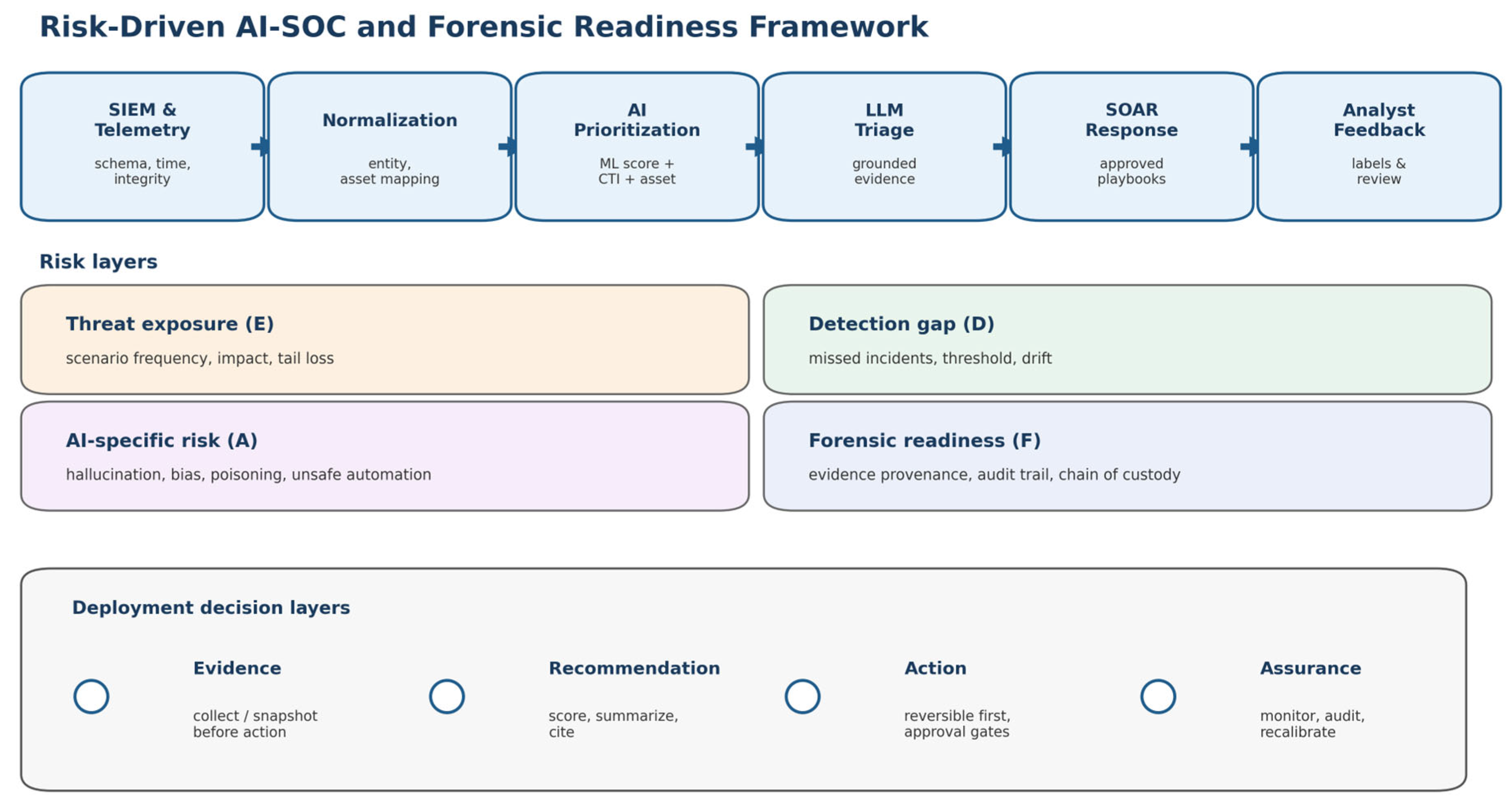
Figure 1 shows the proposed framework. Alerts move from telemetry ingestion to normalization, AI prioritization, LLM-assisted triage, SOAR, and analyst feedback. Around this workflow, the framework tracks threat exposure, detection capability gaps, AI-specific risk, and forensic readiness. The output is not a single automation decision. It is a deployment state: shadow mode, assisted triage, low-risk automation, analyst-approved containment, or rollback to a safer operating mode.
Figure 1.
Risk-driven AI-SOC and forensic readiness framework.
3.2. Risk and Forensic Readiness Components
The composite deployment risk is represented as a weighted score that combines threat exposure, detection gap, AI-specific risk, and forensic readiness risk:
where E is normalized threat exposure, D is the detection capability gap, A is AI-specific risk, F is forensic readiness risk, and the weights sum to one. Threat exposure represents event likelihood and business impact. The detection gap represents missed incidents, threshold errors, and drift. AI-specific risk includes hallucination, prompt injection, poisoning, automation bias, and unsafe tool use. Forensic readiness risk represents the probability that response actions or AI-generated artifacts weaken evidence preservation, provenance, auditability, or reconstruction.
R = w1E + w2D + w3A + w4F,
The method is configurable rather than universal. A critical infrastructure SOC may assign more weight to D and F because missed attacks and weak evidence handling may have severe consequences. A commercial SOC with limited staffing may assign more weight to E and A to balance expected loss, analyst workload, and automation safety. The key point is that deployment decisions should be linked to measurable indicators rather than to a generic belief that more automation is always better.
Equation (1) is an operational aggregation rather than a purely conceptual one, and the normalization and weighting choices are therefore stated explicitly. Each component is mapped to the unit interval by a documented rule before weighting. Threat exposure is normalized against the organization’s stated risk appetite, E = min(1, VaR95/VaR_appetite). The detection gap is the complement of recall at the selected operating threshold, D = 1 − recall. AI-specific risk is measured as the fraction of the monitoring period during which the detector sits below its recall service-level floor, A = breach weeks/total weeks, which makes drift the observable proxy for a broader failure class. Forensic readiness risk is the complement of measured evidence completeness, F = 1 − completeness, where completeness is the proportion of required artifact classes present with intact timestamps and chain-of-custody records at case closure.
Table 2 summarizes the six risk components used in the proposed AI-SOC forensic-readiness model, including the four components included in Equation (1) and the two additional gating constraints. The composite score carries four terms because those four are the ones that vary continuously and are directly estimable from the simulation outputs. The two remaining components of Table 2, analyst workload risk and response automation risk, are evaluated separately as gating constraints rather than as weighted terms, because each can veto a deployment state regardless of how favorable the composite score is. Analyst workload risk is computed as W = max(0, (ρ − ρ*)/(1 − ρ*)) with a target utilization ceiling ρ* = 0.75; in the illustrative scenario W falls from 0.846 in the baseline configuration to 0.100 in the AI-assisted configuration, which is the quantitative form of the claim that queue stability, not detector accuracy, is the binding constraint on the baseline SOC. Response automation risk is assessed as the proportion of playbook actions that are irreversible and not gated by human approval. A SOC that prefers a single scalar may adopt the extended form Rext = w1E + w2D + w3A + w4F + w5W + w6S with weights summing to one; the paper reports the four-term core because separating the gates makes the stop conditions explicit and auditable.
Table 2.
Risk components and practical measurements in the proposed AI-SOC forensic readiness model.
Weights are set by governance decision rather than estimated from data, and the paper makes no claim that any particular weight vector is correct. The illustrative vector used below, (w1, w2, w3, w4) = (0.30, 0.30, 0.20, 0.20), gives equal combined priority to financial exposure and detection capability, with AI-specific and forensic risks carrying half that weight each. A critical infrastructure SOC would be expected to shift weight toward w2 and w4; the weight vector is a declared input to the deployment decision and should be recorded in the audit trail alongside the resulting score.
A worked example ties the four simulation outputs of Section 4 back to the composite score. Taking VaR95 = USD 3.85 M against a declared appetite of USD 8.00 M gives E = 0.481. Recall at the selected threshold of 1.873 is 0.650, giving D = 0.350. The drift trajectory places 20 of 52 weeks below the recall floor, giving A = 0.385. Measured evidence completeness of 0.88 gives F = 0.120. The composite score is therefore R = 0.30(0.481) + 0.30(0.350) + 0.20(0.385) + 0.20(0.120) = 0.350. Under the bands in Table 3, this places the illustrative SOC in the assisted-triage state: the detector may rank, and the LLM may summarize, but no containment action may be executed without analyst approval. The binding constraints are threat exposure and the detection gap, which together contribute 0.249 of 0.350; forensic readiness contributes least and is not the limiting factor in this configuration. This example also illustrates a hazard the framework must acknowledge rather than conceal. The computed score of 0.3503 sits three ten-thousandths above the 0.35 boundary between analyst-approved containment and assisted triage. A marginally better detector, or a slightly more generous risk appetite, would move the SOC into a less restrictive state without any meaningful change in its actual risk posture. A scalar score with hard bands is convenient for governance but brittle at the boundaries, which is why Section 5.3 recommends treating any score within roughly 0.05 of a band edge as a trigger for explicit review rather than as an automatic classification.
Table 3.
Composite risk score bands, deployment states, and gating constraints for AI-SOC deployment.
3.3. Evidence-Preserving SOC Workflow
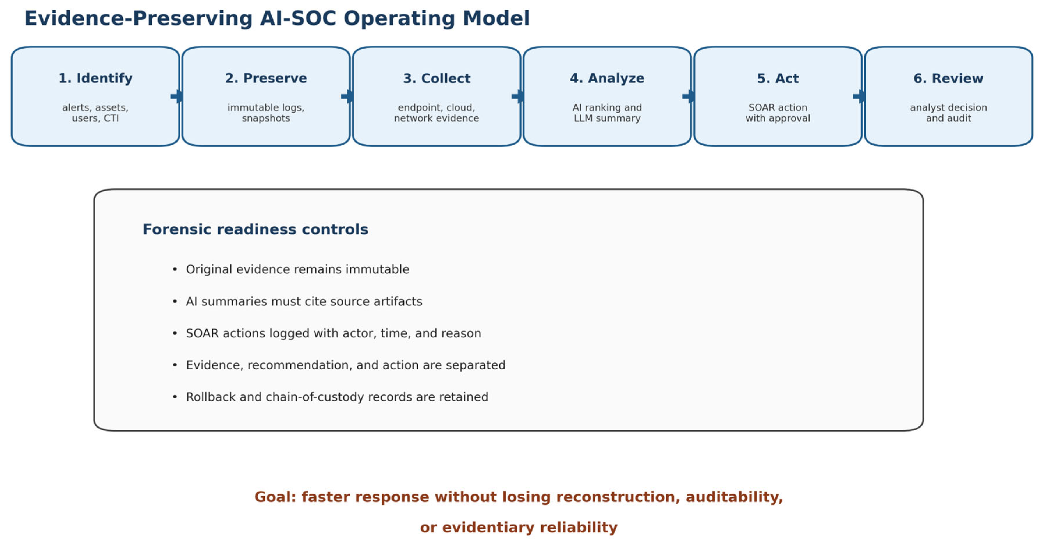
Digital forensic readiness requires that the SOC preserve enough reliable information to reconstruct what happened, when it happened, which systems were affected, which actions were taken, and why those actions were justified. In the proposed workflow, evidence includes logs, endpoint metadata, network events, cloud audit records, identity records, CTI indicators, asset information, case notes, and historical labels. Recommendations include priority scores, LLM summaries, suggested classifications, and proposed response steps. Actions include ticket creation, enrichment, user notification, containment, blocking, isolation, or escalation.
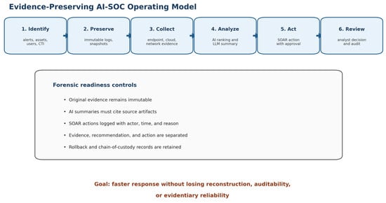
The framework requires an explicit separation between these three layers. Source evidence must remain distinguishable from AI-generated summaries. LLM outputs should cite artifacts and uncertainty, not replace artifacts. SOAR playbooks should collect or snapshot relevant evidence before containment when feasible and proportionate; where delays would materially increase harm, containment may precede preservation provided the exception and its rationale are recorded in the audit trail. Analyst feedback should be stored as operational input but should not automatically become training data until quality review has verified the label. Figure 2 summarizes this evidence-preserving operating model.
Figure 2.
Evidence-preserving AI-SOC operating model for digital forensic readiness.
3.4. Simulation and Evaluation Framework
The complete reproducibility package is provided in the Supplementary Materials and archived on Zenodo under the version DOI reported below. It includes the workbook, Python scripts, generated CSV outputs, article figures, and reported_values.csv, which lists every numerical value quoted in this article together with its manuscript location.
The illustrative evaluation contains four quantitative models. The first is a Monte Carlo annualized loss simulation. Each risk scenario is treated probabilistically: event frequency is drawn from an annual rate, loss severity is drawn from a heavy-tailed distribution, and control effectiveness reduces realized loss. Repeating this process produces mean annualized loss, 95% Value-at-Risk, 99% Value-at-Risk, and loss exceedance curves.
The second model is detector threshold analysis. It starts with model scores and ground-truth labels, then sweeps the decision threshold. For each threshold, it calculates true positives, false positives, precision, recall, F1, true-positive rate, and false-positive rate. ROC and precision-recall curves are both needed because imbalanced security events can make ROC-AUC look strong while false positives still overload analysts.
Throughout this article, MTTR denotes mean time to respond, that is, the interval from alert arrival to the completion of the response action and never mean time to resolution; the same definition is used in the text, the figures, Abbreviations, and the companion workbook. The third model is analyst queueing. Alerts arrive at a rate lambda, and analysts clear them at service rate mu. The M/M/c approximation is not a perfect description of SOC work, which is bursty and heterogeneous, but it illustrates non-linear backlog behavior. When utilization approaches saturation, small increases in alert volume can produce large increases in waiting time. The fourth model is drift and retraining analysis. It estimates recall over time and marks periods when recall falls below a service-level floor.
The Monte Carlo component is specified as follows. Five scenario classes are modeled: phishing and credential theft, ransomware, insider exfiltration, cloud misconfiguration, and supply-chain compromise. Each class is assigned an annual rate of occurrence drawn from a Poisson distribution, and each event draws a single-loss expectancy from a lognormal distribution parameterized by its mean and coefficient of variation, which is the heavy-tailed family used throughout. Realized loss is reduced per event by a control-effectiveness factor drawn from a Beta distribution, so that control performance is itself uncertain rather than fixed; the aggregate annual loss is the sum over all events in all classes. The total event intensity across classes is 22 events per year, dominated by high-frequency, low-severity phishing activity, so essentially every simulated year carries some loss, and the portfolio’s tail behavior is driven by the rare high-severity classes rather than by whether an incident occurs at all. Value-at-Risk is defined as the empirical quantile of the aggregate annual loss distribution over 40,000 iterations, and Tail-VaR as the mean loss conditional on exceeding that quantile. The per-class rate of occurrence, mean single-loss expectancy, coefficient of variation, and Beta control parameters are given in full in Table 4 and in the companion toolkit’s scenario_parameters.csv, and the random seed is fixed, so the distribution regenerates exactly.
Table 4.
Simulation parameters and reproducibility elements.
The detector component uses a synthetic score stream of 10,000 alerts comprising 1000 threat events and 9000 benign events, an imbalance of 1:9. Benign scores are drawn from a standard normal distribution and threat scores from a normal distribution with mean 2.2 and unit standard deviation; this parameterization is what produces the reported ROC-AUC of 0.942 and the operating point at threshold 1.873. Stating the imbalance explicitly matters because it is the quantity that determines how far ROC-AUC can diverge from operational usefulness: the no-skill precision-recall baseline sits at 0.100, so the PR-AUC of 0.750 is the more informative summary and is reported alongside ROC-AUC in Section 4.
The queueing component uses the standard M/M/c model. Expected queue waiting time is computed from the Erlang-C formula, Wq = C(c, a)/(cμ − λ), where a = λ/μ is the offered load in erlangs and C(c, a) is the probability that an arriving alert must wait; standard treatments are given in the queueing literature and the implementation is included in the companion toolkit. MTTR is reported as the sum of three components, MTTR = Wq + 1/μ + T_response, where 1/μ is mean triage handling time, and T_response is mean downstream containment and closure time. Queue waiting time is therefore never reported as MTTR, and the decomposition is given explicitly in Table 5.
Table 5.
Baseline and AI-assisted queueing scenarios, showing the derivation of the reported workload and MTTR changes.
The M/M/c assumption of Poisson arrivals understates waiting time for the bursty, campaign-driven traffic that SOCs actually observe, and it is worth stating the direction and rough magnitude of that error. Under the Allen-Cunneen approximation for G/G/c systems, waiting time scales approximately by (Ca2 + Cs2)/2, where Ca2 and Cs2 are the squared coefficients of variation in interarrival and service times. For plausible SOC values of Ca2 = 2.5 and Cs2 = 1.5, the waiting-time component roughly doubles, moving the baseline configuration from 20.3 to 40.6 min of queue wait and the AI-assisted configuration from 1.9 to 3.8 min, so that end-to-end MTTR moves from 44.3 to 64.6 min in the baseline arm but only from 25.9 to 27.8 min in the AI-assisted arm. Because the correction multiplies a term that is large in the congested baseline and small in the AI-assisted case, the reported MTTR improvement is conservative: burstiness widens the gap rather than narrowing it, and the qualitative conclusion is unchanged. What burstiness does change is the safety margin, since a configuration running at 96.2% utilization has essentially none.
The drift component models detector recall as decaying from an initial value of 0.920 by a weekly amount drawn from a normal distribution with mean 0.010, so that decay is itself stochastic rather than smooth. Retraining every 13 weeks recovers 75% of the performance lost since the start of the period, which represents partial rather than complete recovery, and the recall service-level floor is 0.82. The 13-week retraining cadence and the 75% recovery fraction are chosen governance parameters, not emergent results, and are listed in Table 4.
Table 4 distinguishes simulation inputs from simulation outputs and names, for each row, the script, function, or output file in the companion toolkit that produces or consumes the value. Mean annualized loss is an output of the loss model rather than a parameter, the retraining cadence is an input rather than an emergent property of the plotted drift trajectory; both are placed accordingly. Every value in this table is reproduced by a single command, and the toolkit additionally emits reported_values.csv, which lists every number quoted anywhere in this article together with the section in which it appears.
4. Results
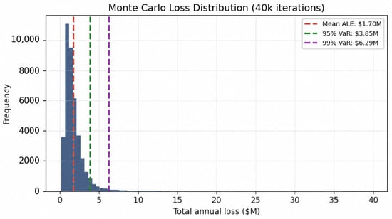
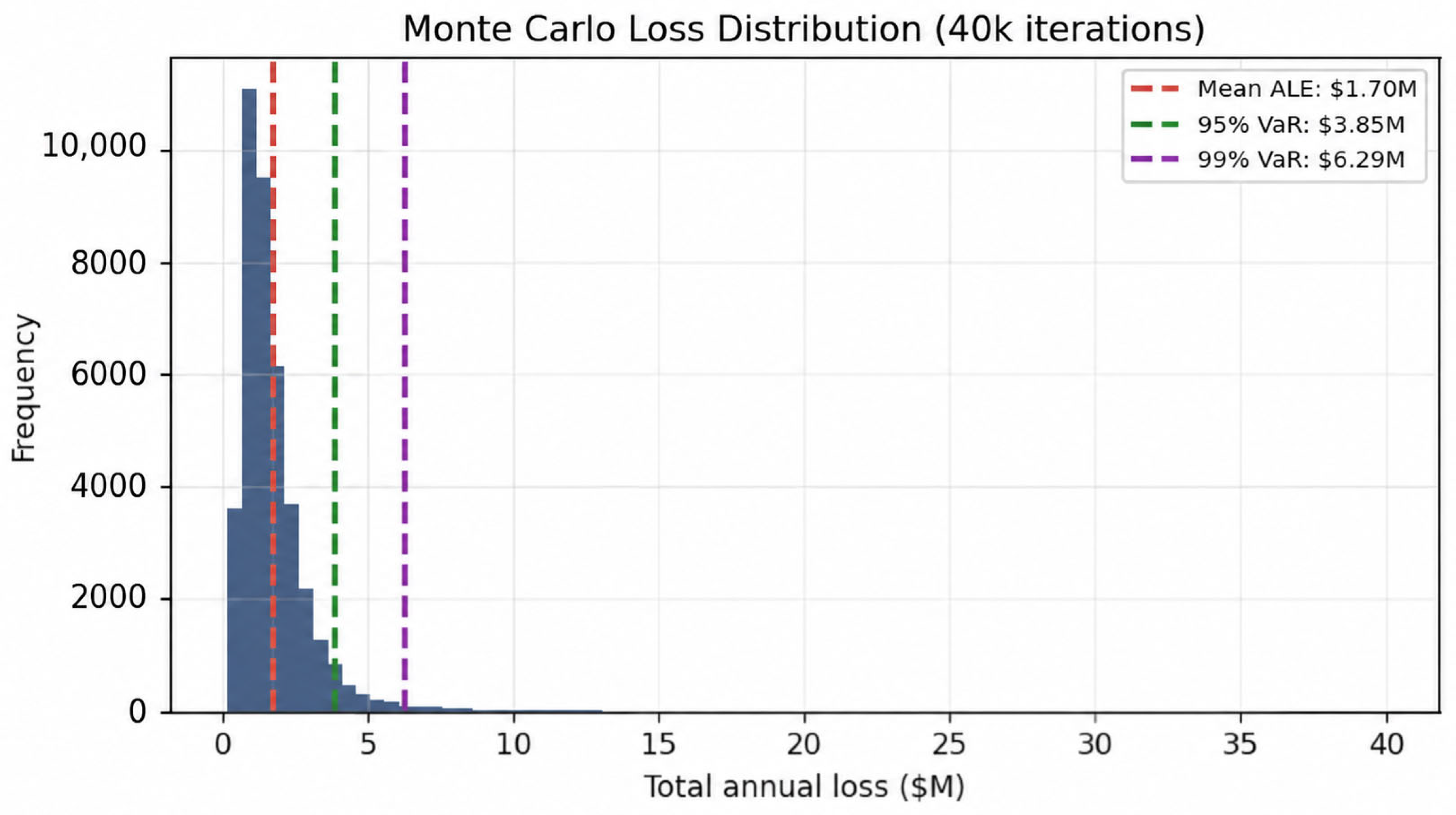
The numerical values in this section are illustrative outputs of the reproducible simulation scenario. They demonstrate the evaluation workflow rather than universal SOC benchmarks. The simulation parameters, workbook structure, and generated figures are intended to support local recalibration with organization-specific incident counts, loss estimates, alert arrival rates, analyst service rates, detector scores, and evidence-retention requirements. Figure 3 shows the distribution of simulated annualized losses.
Figure 3.
Monte Carlo annualized loss distribution for the illustrative AI-SOC scenario. The red, green, and purple dashed vertical lines indicate the mean ALE, 95% VaR, and 99% VaR, respectively.
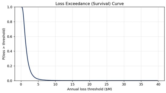
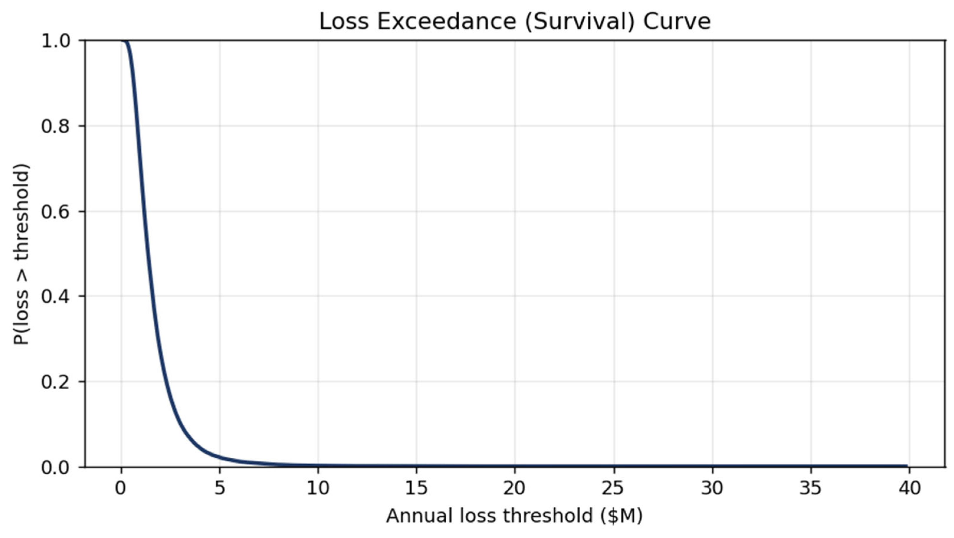
The Monte Carlo simulation produces a mean annualized loss expectancy of USD 1.70 M. The median is USD 1.39 M, the 95% Value-at-Risk is USD 3.85 M, the 99% Value-at-Risk is USD 6.29 M, and the corresponding conditional tail expectations (Tail-VaR) are USD 5.45 M and USD 8.61 M. The gap between a median of USD 1.39 M and a 99% tail of USD 6.29 M is the quantity of interest: a SOC budgeting to the typical year would under-provision against the tail by more than a factor of four. The largest single simulated year reaches USD 39.83 M. Because the modeled portfolio carries a combined event intensity of 22 events per year, essentially no simulated year is loss-free. The corresponding exceedance behavior is shown later in Figure 9. VaR is defined here as the empirical quantile of the simulated annual loss distribution, and Tail-VaR as the mean loss conditional on exceeding that quantile. This result shows why a SOC should not rely only on average expected loss. Rare severe incidents, such as ransomware, identity compromise, or critical infrastructure disruption, may dominate tail risk even when routine alerts dominate everyday workload.
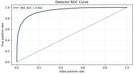
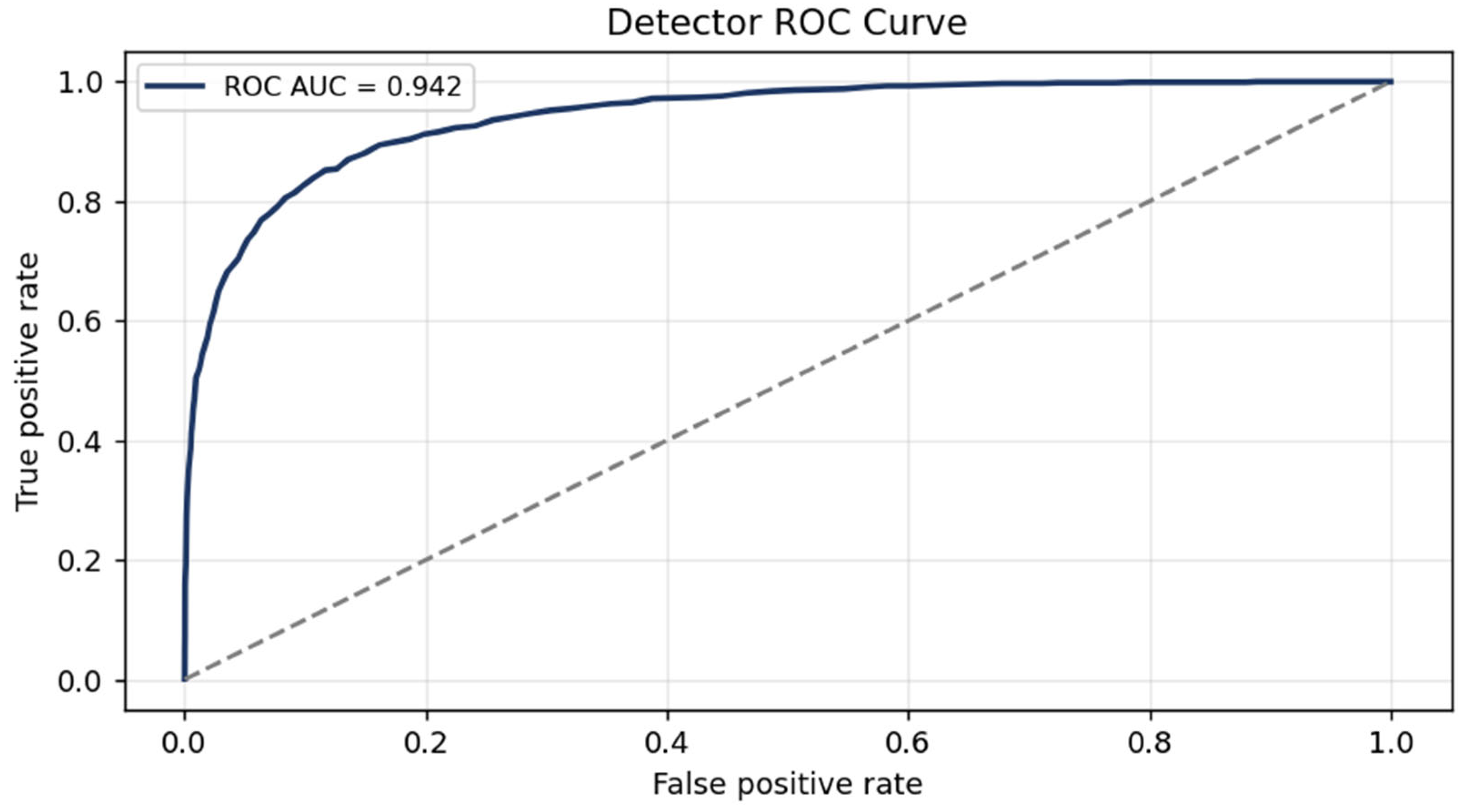
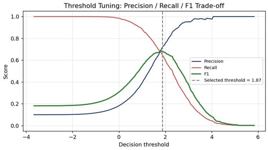
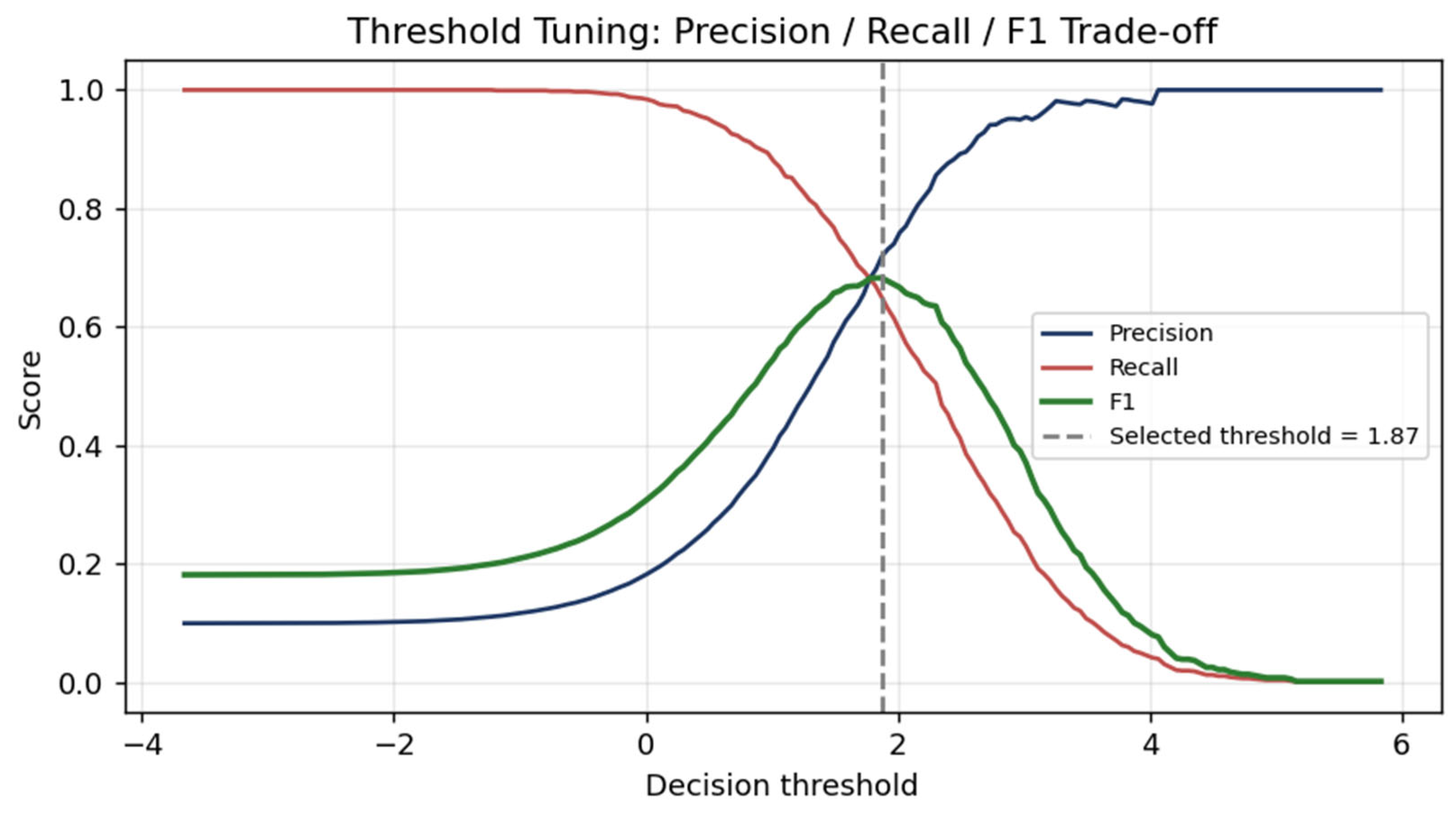
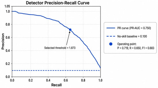
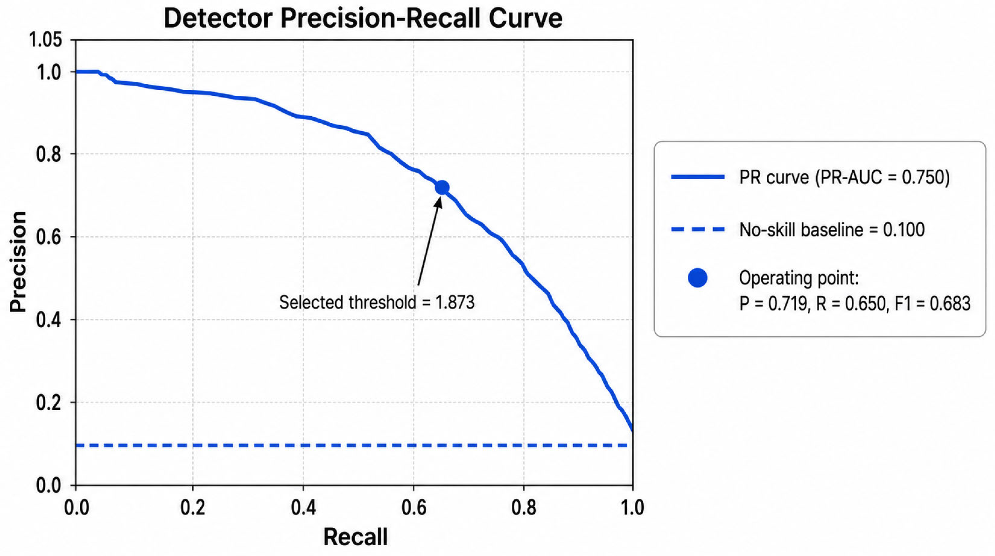
Detector evaluation shows strong rank-ordering in the illustrative dataset (ROC-AUC = 0.942, Figure 4). The operating point selected by maximizing F1 lies at a decision threshold of 1.873 (Figure 5), where precision = 0.719, recall = 0.650, and F1 = 0.683. At that point, the confusion matrix contains 650 true positives, 254 false positives, 350 false negatives, and 8746 true negatives. Because the simulated alert stream is imbalanced (10.0% positives, 1:9), ROC-AUC overstates operational usefulness relative to the precision-recall view reported in Figure 6, where PR-AUC = 0.750 against a no-skill baseline of 0.100.
Figure 4.
ROC curve for the simulated detector. The dashed diagonal line indicates the no-skill reference line.
Figure 5.
Threshold tuning for precision, recall, and F1-score. The dashed vertical line indicates the selected decision threshold.
Figure 6.
Detector precision-recall curve for the simulated alert stream. The marker indicates the selected operating point; the dashed horizontal line shows the no-skill baseline given by the positive-class prevalence; and the annotation reports the selected threshold.
The gap between an ROC-AUC of 0.942 and an F1 of 0.683 is precisely the effect the methodology anticipates: strong separability does not by itself protect analysts from false-positive load. The operational reading is blunter still. At the F1-maximizing threshold, the detector misses 350 of 1000 genuine threats while still sending 254 false positives to analysts, which is why the article treats threshold choice as a governance decision rather than a metric to be maximized. The main message is therefore operational rather than purely statistical. A threshold that maximizes F1 may still be unsafe if it floods analysts, while a threshold that reduces false positives may be unacceptable for high-criticality assets. Threshold selection should therefore be a management and forensic readiness decision as well as a model-performance decision.
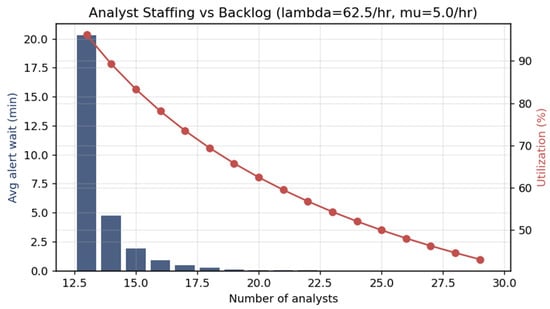
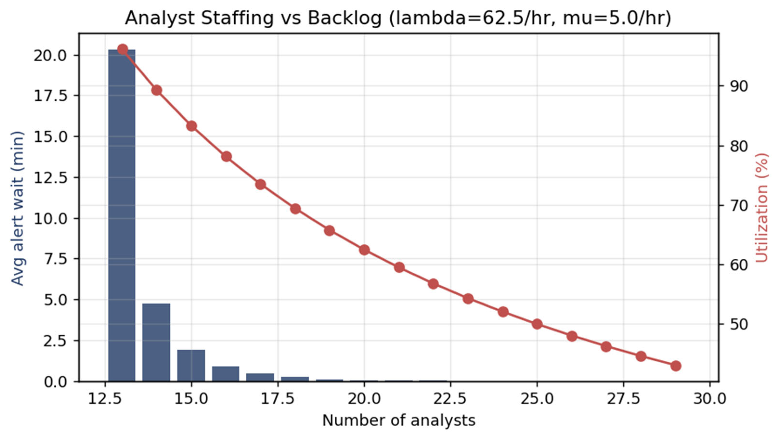
The queueing model explains why workload reduction matters. SOC utilization should not be managed at maximum capacity. As utilization approaches saturation, alert waiting time increases non-linearly. AI can help by deduplicating alerts, enriching evidence before analysts open cases, and ranking incidents by risk. However, if AI lowers detection thresholds without reducing false positives, it can make workload risk worse. Detector thresholds and queueing capacity must therefore be tuned together, as illustrated in Figure 7 by the resulting analyst staffing and backlog behavior. In the illustrative scenario, these combined effects correspond to an approximately 38% reduction in manual triage workload and a reduction in MTTR from about 44 to 26 min. Table 5 documents how both figures are obtained. Workload is defined as the offered load presented to Tier-1 triage, measured either as alerts requiring manual handling per hour (62.5 to 38.75) or equivalently as offered analyst-hours per hour (12.50 to 7.75 erlangs); both definitions give the same 38% reduction. MTTR is decomposed as queue waiting time plus triage handling time plus downstream response time, so that queue waiting time is never conflated with end-to-end MTTR. Consistent with the rest of this section, these are demonstration outputs of the reproducible simulation rather than universal benchmarks.
Figure 7.
Analyst staffing and backlog behavior under queueing assumptions.
The 38% workload reduction and the MTTR change are therefore not independent claims. Both follow from the same two inputs, the reduction in manual triage volume and the resulting fall in utilization, and the non-linearity of the Erlang-C waiting term is what converts a 38% volume reduction into a 42% MTTR reduction. Almost all of the MTTR gain comes from the queue term, which collapses from 20.3 to 1.9 min, while the handling and response components are held constant across both arms precisely so that the queueing effect is not confounded with an assumed improvement in analyst speed.
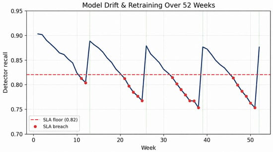
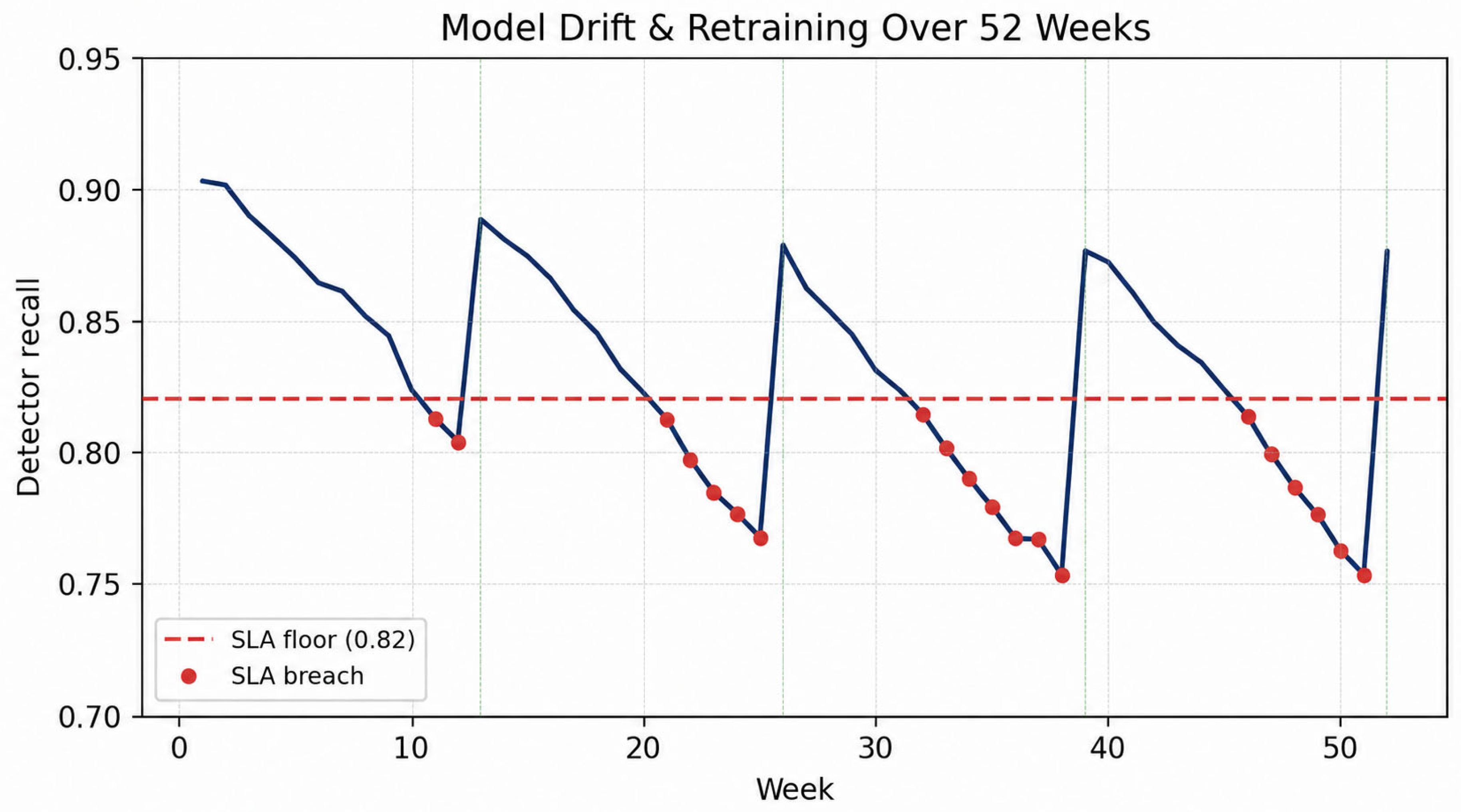
The drift trajectory in Figure 8 is generated with an initial recall of 0.920, a stochastic weekly decay averaging 0.010, and retraining at weeks 13, 26, 39, and 52 that recovers 75% of the performance lost since the start of the period. Recall falls to a minimum of 0.753 and 20 of 52 weeks lie below the 0.82 floor. Because recovery is partial rather than complete, the trajectory does not return to its initial value after each retraining event and the SOC spends a substantial minority of the year in breach; this is a deliberate modeling choice, since a model that fully recovered on every retraining cycle would understate the governance burden of drift. The retraining cadence and recovery fraction are chosen governance parameters and are stated explicitly in Table 4 rather than left to be inferred from the chart. The drift trajectory shows that AI performance is time-dependent. A detector validated once may fall below recall requirements when attacker behavior, infrastructure, user activity, or alert distributions change. Recall service-level breaches should be treated as governance events rather than only technical model errors. They should trigger review of thresholds, training data quality, analyst feedback, detection coverage, and automation scope before response actions are expanded.
Figure 8.
Model-drift trajectory with retraining events and recall service-level breaches. The blue line shows detector recall, the red dashed line shows the recall SLA floor, red markers indicate SLA breaches, and pale vertical lines indicate retraining events.
Returning to the loss model, because the modeled portfolio carries a combined event intensity of 22 events per year, essentially no simulated year is loss-free, and the exceedance curve in Figure 9 therefore begins at unity rather than at a lower intercept.
Figure 9.
Annual loss exceedance curve from the Monte Carlo simulation. The curve shows the probability that total annual loss exceeds each threshold and illustrates the long-tail exposure of the simulated AI-SOC risk scenario.
Recall is therefore treated as the minimum drift trigger, not the only drift trigger. In an operational deployment, retraining or rollback should also be considered when feature distributions, score distributions, asset mix, alert-source composition, or analyst override patterns shift materially. Practical triggers include a population-stability-index warning for high-value features, a Kolmogorov–Smirnov or Jensen–Shannon divergence warning for score distributions, a sudden rise in low-confidence LLM summaries, or a sustained increase in analyst overrides. These additional indicators are not used to generate the illustrative recall curve, but they are included in the governance rule so that drift monitoring is not reduced to a single recall threshold.
5. Discussion
5.1. Operational and Forensic Interpretation
The framework supports three operational decisions. The first is where to set the detection threshold. A risk-sensitive SOC may choose different thresholds for different asset classes. A low-confidence signal on a non-critical workstation may remain in routine review, while the same signal on a domain controller, production identity provider, or evidence repository may be escalated. This is why the priority score includes CTI relevance, asset criticality, and forensic readiness rather than treating all alerts equally.
The second decision is whether to invest in analysts, automation, or model improvement. If the queueing model shows saturation, redistributing analysts or improving enrichment may reduce risk faster than tuning the model. If false negatives dominate residual exposure, detection engineering and retraining may be more valuable than additional SOAR playbooks. If evidence gaps dominate forensic readiness risk, log integrity, retention, timestamp quality, and immutable storage may be more urgent than faster containment.
The third decision is how to govern AI over time. A model that performs well during initial validation should still be monitored for calibration, drift, and changing error patterns. A playbook that is safe during a tabletop exercise should still be tested for rollback and evidence impact. An LLM assistant that gives useful summaries should still be evaluated for unsupported claims, source confusion, and prompt-injection exposure. AI in the SOC is therefore an operational control that requires release management, continuous monitoring, and audit.
It is worth returning to the six research streams identified in Section 2, because the results speak to the specific gap named for each. For alert fatigue and SOC work, the queueing results give the missing quantitative form: workload is not merely a human factor but a stability property, and the baseline configuration at 96.2% utilization is shown in Section 5.3 to be one 5% perturbation away from unbounded backlog. For ML detection and prioritization, the gap was that model metrics are rarely mapped to residual loss or queue stability; the threshold-queue coupling reported in Section 5.3 supplies exactly that mapping and shows that a nine-point recall improvement can saturate the queue. For CTI and vulnerability context, the framework uses asset criticality as a threshold modifier rather than a post-triage annotation, which is why the composite score admits different operating points for different asset classes.
For SOAR automation, the gap was that automation can act before evidence is preserved; the deployment states in Table 3 make evidence snapshot a gating condition rather than a recommended practice, and response automation risk is treated as a veto rather than a weighted term. For LLM assistants, the gap was hallucination and injection through retrieved text; these enter the composite score through the AI-specific risk term and through the grounding requirements in Section 3.3. For digital forensics and forensic readiness, the gap was that evidence quality is weakened by AI summaries and automated containment; forensic readiness risk is the one term in Equation (1) that can force rollback on its own. In the illustrative configuration, the binding constraints proved to be threat exposure and the detection gap rather than forensic readiness, but that is a property of this scenario and not a general finding.
5.2. Risk-Control Matrix and Forensic Readiness Controls
Table 6 shows that AI-enabled SOC systems introduce both technical and forensic risks. False-negative prioritization can hide real incidents. False-positive overload can weaken analyst attention. LLM hallucination can insert unsupported claims into incident records. Unsafe SOAR actions can disrupt business services or modify evidence. Evidence contamination and weak provenance are especially important for the digital-forensics context because they affect later reconstruction and auditability.
Table 6.
Example risk-control matrix for AI-enabled SOC deployment and forensic readiness.
To make the LLM-related controls measurable rather than purely conceptual, the framework now treats each LLM-assisted triage output as an auditable object. The output must contain: (i) cited source artifacts, (ii) an uncertainty statement expressed as evidence coverage rather than model confidence alone, (iii) a contradiction or unsupported-claim flag, and (iv) an indication of whether any retrieved text contained instruction-like content. LLM text may support prioritization and reporting only when grounding coverage is sufficient; it cannot by itself trigger containment or other irreversible SOAR action. The numerical decision rules in Table 7 are proposed release criteria rather than empirically derived thresholds. They are set deliberately conservatively for an initial deployment, on the principle that an assistant whose claims cannot be traced to artifacts should not influence escalation, and they are expected to be recalibrated locally once a SOC has measured its own grounding and attribution rates. The single exception is the prompt-injection rule, which is set at zero tolerance because a successful injection compromises the instruction hierarchy itself rather than degrading output quality by a measurable margin.
Table 7.
Measurable LLM-control indicators for a controlled validation protocol.
Forensic readiness is also made measurable. Table 8 lists indicators intended for case-level audit, which can be calculated from ticket records, immutable log storage, evidence manifests, and SOAR action logs. The numerical values below are illustrative demonstration targets for the workflow rather than live SOC measurements; they show how the proposed evidence-preserving workflow would be compared with a baseline AI/SOAR workflow during local validation.
Table 8.
Forensic readiness indicators for baseline-versus-proposed workflow validation.
Because evidence completeness is the input to the forensic readiness term of Equation (1), the two illustrative columns can be carried through the composite score to show what the workflow change would mean for a deployment decision rather than only for an audit metric. Baseline completeness of 0.62 gives F = 0.380 and proposed completeness of 0.88 gives F = 0.120. Holding the other three components at their Section 3.2 values, the composite score falls from 0.402 to 0.350 under the balanced weight vector, which is an improvement but not one large enough to change the deployment state. Section 5.3 shows that the workflow change does move the state under three of the five weight profiles examined: the detection-heavy, forensic-heavy and equal-weight vectors all shift the SOC from assisted triage into analyst-approved containment, with the forensic-heavy vector producing the largest movement, from 0.395 to 0.291. The honest reading is therefore conditional: adopting the evidence-preserving workflow expands permitted automation in most but not all of the weightings considered, and for a SOC on the balanced or loss-heavy vectors its benefit in this illustrative configuration is a lower residual risk score rather than an unlocked automation tier. Both figures are demonstration targets, not measured outcomes, and the comparison should be repeated with audited case data before it is used to justify a change in automation scope.
5.3. Sensitivity Analysis and Calibration
A useful extension of the evaluation is sensitivity analysis. The SOC should not ask only whether the model performs well under one baseline. It should ask which assumptions change the result most strongly. In many environments, the most sensitive variables are incident severity, false-negative cost, analyst service rate, alert arrival rate, decay rate of model recall, and evidence-completeness requirements.
Sensitivity is reported quantitatively for the parameters that drive the headline outputs, using one-at-a-time perturbations of plus or minus 5% around the illustrative configuration. Table 9 gives the resulting MTTR range. The dominant finding is not the size of any individual swing but the asymmetry between the two configurations: the baseline SOC, running at 96.2% utilization, is driven into queue saturation by a 5% adverse move in arrival rate, service rate, or analyst count, so its MTTR is unbounded in three of four directions. The AI-assisted configuration at 77.5% utilization responds smoothly, with a worst-case swing of 3.0 min. For the loss model, mean annualized loss is exactly linear in each scenario frequency and in each control-effectiveness complement; a 10% change in either produces a 10% change in that class’s contribution to ALE. The tail quantiles do not follow the mean: as Table 10 shows, they respond super-linearly to the severity dispersion parameter and sub-linearly to frequency, so the ranking of assumptions by influence differs depending on whether the SOC is managing expected loss or tail exposure.
Table 9.
One-at-a-time sensitivity of MTTR to the principal queueing assumptions (plus or minus 5% perturbation).
Table 10.
Illustrative Monte Carlo loss sensitivity under one-at-a-time parameter perturbations.
The threshold-queue coupling can be quantified on the same basis, and it sharpens the point made in Section 2 about detector metrics being reported without queue consequences. Lowering the decision threshold from 1.873 to 1.635 raises recall from 0.650 to 0.721, an apparent detection improvement of seven percentage points, but raises the alert rate presented to analysts from 62.5 to 79.9 per hour, which drives utilization to 1.23 at the baseline staffing of 13 and saturates the queue entirely. Lowering it further, to 1.396, raises recall to 0.791 and utilization to 1.58. Conversely, raising the threshold to 2.112 cuts the alert rate to 48.8 per hour, brings utilization down to 0.751, and reduces MTTR to 24.9 min, but at the cost of recall falling to 0.557. A threshold change that improves recall by seven percentage points can therefore make the SOC strictly worse, which is the interaction the composite score in Equation (1) is designed to expose and which no single-stream evaluation would surface.
The sensitivity of the loss estimates themselves is reported in Table 10, which gives one-at-a-time illustrative perturbations of the main Monte Carlo assumptions. Each row is a separate 40,000-iteration run of the loss model under the fixed seed recorded in the companion workbook, so the perturbed values are simulated rather than obtained by rescaling the baseline outputs. The values are not presented as external benchmarks; they show how the simulation workbook should be used to test whether a deployment decision is stable when frequency, severity and control-effectiveness assumptions vary.
Two features of Table 10 matter more than the individual magnitudes. First, frequency and severity do not act on the distribution in the same way. Multiplying every loss by a constant rescales the mean and every quantile by that same constant, so the severity-scale rows move by exactly ten per cent throughout; changing how often events occur moves the mean by ten per cent but moves VaR95 by 6.8% and VaR99 by only 5.8%, because the tail is dominated by the severity of individual large events rather than by their count. A SOC that reduces incident frequency by a tenth should therefore not expect its 99% tail to fall by a tenth. Second, dispersion moves the tail while leaving the mean almost untouched: a 10% increase in the coefficient of variation raises VaR99 by 4.6% and the mean by 0.1%. This is the quantitative form of the argument that a SOC should not manage to average expected loss, and it identifies severity dispersion as the assumption most deserving of local calibration effort when tail exposure is the concern.
Because Equation (1) is a governance aggregation, the weight vector must also be tested. Table 11 shows that the illustrative score remains below rollback and shadow-mode thresholds under several plausible weight configurations, but it can move between assisted triage and analyst-approved containment when the score is close to a decision boundary. This is why the paper treats the weight vector as an auditable governance input rather than as an estimated model parameter.
Table 11.
Weight-configuration sensitivity of the composite deployment score.
The sensitivity that matters here is not the spread of the score, which is modest, but its position relative to a band boundary. Under the baseline workflow, every weight profile leaves the SOC in assisted triage; under the proposed evidence-preserving workflow, three of the five move it into analyst-approved containment. The balanced vector is the marginal case, producing 0.350 against a boundary at 0.350, and the loss-heavy vector does not move the state at all. Two conclusions follow. The weight vector is a decision input of the same standing as the measurements and should be recorded in the audit trail alongside the resulting score. And because a score can sit arbitrarily close to a boundary, any result within roughly 0.05 of a band edge should trigger explicit governance review rather than automatic promotion or demotion. Alongside these quantitative perturbations, Table 12 records the qualitative calibration signals that should be tracked during local validation.
Table 12.
Qualitative calibration signals for the AI-SOC risk and forensic readiness model (companion to the quantitative sensitivity results in Table 9).
Calibration should begin with data the SOC already owns. Incident-ticket counts can estimate annual rates of occurrence. Post-incident cost reports can estimate severity distributions. SIEM exports can provide alert arrival rates by hour, source, and severity. Ticket timestamps can estimate analyst service rates. Historical model scores or rule-triggered alerts can support threshold curves. Forensic calibration requires log-retention checks, timestamp-quality checks, artifact-completeness checks, and audit-trail coverage.
5.4. Component Analysis and Ablation Logic
This section sets out the ablation logic of the framework: it explains why the framework combines several components rather than relying on a single model. It is a structured statement of expected contribution, not a controlled ablation experiment, since no component was removed from a running system and re-measured. Table 13 summarizes the expected effect of removing or adding components. The entries are expected effects derived from the framework’s design rather than measured differences and are labeled as such. A quantitative ablation, in which each component is removed from the pipeline and the composite score recomputed, is left to the live-SOC validation identified in Section 7.
Table 13.
Expected component contributions (ablation logic, not measured ablation results) for AI-SOC deployment.
5.5. Threats to Validity
Internal validity is limited by simulation assumptions. The results depend on scenario frequencies, severity distributions, detector scores, alert arrival rates, service rates, and drift assumptions. The one-at-a-time sensitivity analysis reported in Section 5.3 bounds the effect of the principal assumptions on the reported outputs, but it does not establish external validity and does not replace local calibration; the component analysis in Section 5.4 is qualitative and is not a controlled ablation experiment. External validity is limited because SOCs differ by sector, maturity, staffing, telemetry, legal obligations, and attacker interest. Construct validity is limited because metrics such as AUC, F1, or MTTR do not fully capture analyst trust, evidence quality, or reconstruction reliability. Data validity is limited by incomplete labels, inconsistent closure notes, and changing detection rules. LLM validity is limited because retrieval grounding reduces hallucination but does not eliminate source confusion or prompt injection. These threats support the article’s main argument: AI-SOC deployment should proceed through measured stages with stop conditions, audit trails, and human approval gates.
The absence of validation on operational SOC data is the strongest external-validity limitation of the study. The detector experiment uses synthetic scores rather than a public intrusion-detection or SOC dataset; the LLM controls are specified as measurable release criteria rather than tested against a live assistant; and the forensic readiness indicators are an illustrative audit rubric rather than measured outcomes from a deployed SOAR environment. Consequently, the numerical values should be interpreted as a reproducible demonstration of the decision method, not as evidence that the method improves outcomes in any specific SOC. Public-dataset detector validation, controlled LLM prompt-injection experiments, and live or retrospective DFIR case audits are required before the framework can support sector-level claims.
6. Practical Recommendations
First, deploy AI in shadow mode before it changes routing or response. Shadow mode provides evidence about model quality, calibration, missing data, retrieval weaknesses, analyst trust, and evidence coverage.
Second, automate enrichment before containment. Related-alert search, asset lookup, CTI enrichment, ticket creation, and draft summaries are safer early targets than endpoint isolation or blocking.
Third, preserve evidence before automated response. When feasible and proportionate, the SOC should snapshot relevant logs, endpoint metadata, process details, user activity, network indicators, and ticket context before containment actions are executed. This ordering is a default, not an absolute rule. Where delay would materially increase harm, for example active ransomware encryption, ongoing exfiltration, or lateral movement toward a domain controller, immediate containment properly takes precedence over preservation. In those cases, the framework requires that the exception be recorded in the audit trail with the acting identity, the time, the justification for overriding the preservation step, and whatever partial evidence could be captured, so that the gap in the evidentiary record is itself documented rather than silent.
Fourth, treat thresholds as management decisions. The best F1 threshold is not automatically the best SOC threshold. Thresholds should reflect asset criticality, threat context, analyst capacity, business impact, and evidence-preservation requirements.
Fifth, make evidence provenance visible. Analysts should be able to see why an alert was ranked, which CTI sources were used, which artifacts supported an LLM summary, and which SOAR actions were taken.
Sixth, monitor drift, feedback quality, and forensic readiness. Retraining is useful only when labels are reliable, and the new model is validated before deployment. Evidence-completeness checks and chain-of-custody logs should be monitored alongside accuracy metrics.
Seventh, report AI-SOC performance through risk and forensic metrics. Dashboards should include expected loss, Value-at-Risk, queue waiting time, analyst utilization, drift breaches, override rates, unsafe automation attempts, missing-evidence rates, and provenance-check failures.
7. Conclusions
This article reframed AI-enabled SOC deployment as a risk-analysis and forensic readiness problem. Instead of focusing only on the architecture of AI components, it proposed a framework that connects threat exposure, detection capability, analyst workload, model drift, LLM governance, SOAR automation, evidence provenance, and incident reconstruction.
The proposed framework combines Monte Carlo annualized loss simulation, detector threshold analysis, analyst queueing, drift/retraining modeling, and forensic readiness controls. In the illustrative evaluation, the framework produced a mean annualized loss expectancy of USD 1.70 M, a 95% Value-at-Risk of USD 3.85 M, a 99% Value-at-Risk of USD 6.29 M, a detector ROC-AUC of 0.942 and PR-AUC of 0.750, precision 0.719, recall 0.650 and F1 0.683 at the selected threshold of 1.873, a triage workload reduction of about 38%, and an MTTR reduction from about 44 to 26 min. These values are not universal claims. They demonstrate how a SOC can connect AI performance to operational risk, financial exposure, and evidence-preserving incident response.
The main contribution is not a claim that AI always reduces SOC risk. The contribution is a practical method for measuring when AI reduces risk, when it transfers risk, and when forensic readiness requires human approval, evidence preservation, or automation rollback. Future work should validate the framework on live SOC data, test it under adversarial conditions, evaluate analyst trust and decision quality, and develop standard reporting templates for AI-SOC risk and forensic readiness dashboards.
In particular, the next validation step should use a public intrusion-detection dataset for detector benchmarking, a controlled benign-versus-malicious retrieval corpus for LLM grounding and prompt-injection testing, and retrospective SOC or DFIR cases for measuring evidence completeness, provenance coverage, timestamp integrity and chain-of-custody completeness against a baseline workflow.
Supplementary Materials
The companion materials for this article are archived on Zenodo under the title “Companion to the AI-SOC Risk Model workbook and simulation toolkit”. The version corresponding to this article is publicly available at https://zenodo.org/records/22012440 (accessed on 19 August 2026). This version DOI should be used when citing the materials or verifying the values reported here, because it resolves to the exact deposit from which these results were generated and will continue to do so if the toolkit is later updated. The deposit comprises AI_SOC_Risk_Model_v2.zip, which contains the complete package, together with README.md, CHANGELOG.md, and reported_values.csv provided separately for direct inspection. Every figure and every numerical value in this article is produced by a single command, python run_article_outputs.py, which draws on the model definitions in soc_sim.py and the risk, sensitivity, and deployment-state extensions in soc_risk.py. That command regenerates Figure 3, Figure 4, Figure 5, Figure 6, Figure 7, Figure 8 and Figure 9 and writes reported_values.csv, an explicit list of every number quoted in this article together with the section or table in which it appears; any value in the manuscript that does not appear in that file should be treated as an error. Figure 1 and Figure 2 are conceptual diagrams and are not simulation outputs. The accompanying Excel workbook, AI_SOC_Risk_Model.xlsx, implements Equation (1) and reproduces the composite risk scores reported in Section 3.2 and Section 5.2. Random seeds are fixed in the source: 42 for the loss model, 7 for the detector, and 3 for the drift trajectory, so that the reported values regenerate exactly. The materials were produced with Python 3.12, NumPy 2.4, pandas 3.0, and Matplotlib 3.10, with exact pinned versions in requirements.txt. The README documents the execution order and the expected console output. All data are synthetic and illustrative; no operational SOC telemetry, incident records, or customer data are included or used.
Author Contributions
Conceptualization, O.T. and D.P.-T.; methodology, O.T., D.P.-T. and A.D.; software and simulation design, O.T. and A.D.; validation, D.P.-T., A.D., Z.H. and I.B.; formal analysis, O.T. and D.P.-T.; investigation, O.T., D.P.-T., A.D., Z.H. and I.B.; writing—original draft preparation, O.T.; writing—review and editing, O.T., D.P.-T., A.D., Z.H. and I.B.; visualization, O.T.; supervision, O.T. and D.P.-T.; project administration, O.T. All authors have read and agreed to the published version of the manuscript.
Funding
The idea for this article was inspired by the AI-Driven Cybersecurity: Opportunities and Challenges project, funded by the Swedish Institute, 00285/2025, and by the Future Industry Program at Halmstad University.
Institutional Review Board Statement
Not applicable.
Informed Consent Statement
Not applicable.
Data Availability Statement
The data and code presented in this study are openly available on Zenodo at https://doi.org/10.5281/zenodo.22012440. The deposit contains the simulation code, generated datasets and figures, the companion Excel risk model, README.md, CHANGELOG.md, and reported_values.csv, which lists every numerical value quoted in this article together with the section or table in which it appears. All data are synthetic and illustrative; no operational SOC telemetry, incident records, or customer data were included or used. The default parameters are demonstration values rather than benchmarks and should be recalibrated before operational use.
Acknowledgments
During the preparation of this manuscript, the authors used GPT-5 for grammar and spelling checks and to assist with the generation of schematic figures. The authors reviewed and edited all content as needed and take full responsibility for the publication content.
Conflicts of Interest
The authors declare no conflicts of interest. The funders had no role in the design of the study; in the collection, analyses, or interpretation of data; in the writing of the manuscript; or in the decision to publish the results.
Abbreviations
The following abbreviations are used in this manuscript:
| AI | Artificial intelligence |
| ALE | Annualized loss expectancy |
| CTI | Cyber threat intelligence |
| CVSS | Common Vulnerability Scoring System |
| DFIR | Digital forensics and incident response |
| LLM | Large language model |
| MTTR | Mean time to respond |
| PR-AUC | Area under the precision-recall curve |
| ROC-AUC | Area under the receiver operating characteristic curve |
| SIEM | Security information and event management |
| SLA | Service-level agreement |
| SOAR | Security orchestration, automation, and response |
| SOC | Security Operations Center |
| Tail-VaR | Tail Value-at-Risk (conditional tail expectation) |
| VaR | Value-at-Risk |
References
- Tariq, S.; Chhetri, M.B.; Nepal, S.; Paris, C. Alert fatigue in security operations centres: Research challenges and opportunities. ACM Comput. Surv. 2025, 57, 224. [Google Scholar] [CrossRef] [Scilit]
- Nelson, A.; Rekhi, S.; Souppaya, M.; Scarfone, K. Incident Response Recommendations and Considerations for Cybersecurity Risk Management: A CSF 2.0 Community Profile; NIST Special Publication 800-61 Revision 3; National Institute of Standards and Technology: Gaithersburg, MD, USA, 2025. [Google Scholar] [CrossRef] [Scilit]
- Kent, K.; Chevalier, S.; Grance, T.; Dang, H. Guide to Integrating Forensic Techniques into Incident Response; NIST Special Publication 800-86; National Institute of Standards and Technology: Gaithersburg, MD, USA, 2006. [Google Scholar] [CrossRef] [Scilit]
- ISO/IEC 27037:2012; Information Technology—Security Techniques—Guidelines for Identification, Collection, Acquisition and Preservation of Digital Evidence. International Organization for Standardization: Geneva, Switzerland, 2012.
- Casey, E. Digital Evidence and Computer Crime: Forensic Science, Computers and the Internet, 3rd ed.; Academic Press: Waltham, MA, USA, 2011. [Google Scholar]
- Garfinkel, S.L. Digital forensics research: The next 10 years. Digit. Investig. 2010, 7, S64–S73. [Google Scholar] [CrossRef] [Scilit]
- Apruzzese, G.; Laskov, P.; Montes de Oca, E.; Mallouli, W.; Rapa, L.B.; Grammatopoulos, A.V.; Di Franco, F. The role of machine learning in cybersecurity. Digit. Threats Res. Pract. 2023, 4, 8. [Google Scholar] [CrossRef] [Scilit]
- Ban, T.; Takahashi, T.; Ndichu, S.; Inoue, D. Breaking alert fatigue: AI-assisted SIEM framework for effective incident response. Appl. Sci. 2023, 13, 6610. [Google Scholar] [CrossRef] [Scilit]
- Gelman, B.; Taoufiq, S.; Vörös, T.; Berlin, K. That escalated quickly: An ML framework for alert prioritization. arXiv 2023, arXiv:2302.06648. [Google Scholar] [CrossRef] [Scilit]
- Sun, N.; Zhang, J.; Ding, M.; Xu, W.; Mo, X.; Tai, Y.; Jiang, J. Cyber threat intelligence mining for proactive cybersecurity defense: A survey and new perspectives. IEEE Commun. Surv. Tutor. 2023, 25, 1748–1774. [Google Scholar] [CrossRef] [Scilit]
- MITRE. MITRE ATT&CK: Design and Philosophy. Available online: https://attack.mitre.org/ (accessed on 17 July 2026).
- FIRST. Common Vulnerability Scoring System Version 4.0 Specification Document. Available online: https://www.first.org/cvss/ (accessed on 17 July 2026).
- Kinyua, J.; Awuah, L. AI/ML in security orchestration, automation and response: Future research directions. Intell. Autom. Soft Comput. 2021, 28, 527–545. [Google Scholar] [CrossRef] [Scilit]
- Norem, S.; Rice, A.E.; Erwin, S.; Bridges, R.A.; Oesch, S.; Weber, B. A mathematical framework for evaluation of SOAR tools with limited survey data. arXiv 2021, arXiv:2112.00100. [Google Scholar] [CrossRef] [Scilit]
- Ismail; Kurnia, R.; Brata, Z.A.; Nelistiani, G.A.; Heo, S.; Kim, H.; Kim, H. Toward robust security orchestration and automated response in security operations centers with a hyper-automation approach using agentic artificial intelligence. Information 2025, 16, 365. [Google Scholar] [CrossRef] [Scilit]
- Habibzadeh, A.; Feyzi, F.; Atani, R.E. Large language models for security operations centers: A comprehensive survey. arXiv 2025, arXiv:2509.10858. [Google Scholar] [CrossRef] [Scilit]
- Srinivas, S.; Kirk, B.; Zendejas, J.; Espino, M.; Boskovich, M.; Bari, A.; Dajani, K.; Alzahrani, N. AI-augmented SOC: A survey of LLMs and agents for security automation. J. Cybersecur. Priv. 2025, 5, 95. [Google Scholar] [CrossRef] [Scilit]
- Singh, R.; Tariq, S.; Jalalvand, F.; Chhetri, M.B.; Nepal, S.; Paris, C.; Lochner, M. LLMs in the SOC: An empirical study of human-AI collaboration in security operations centres. arXiv 2025, arXiv:2508.18947. [Google Scholar] [CrossRef] [Scilit]
- Saju, M.H.; Azim, A. Toward autonomous SOC operations: End-to-end LLM framework for threat detection, query generation, and resolution in security operations. arXiv 2026, arXiv:2604.27321. [Google Scholar] [CrossRef] [Scilit]
- Papernot, N.; McDaniel, P.; Sinha, A.; Wellman, M. SoK: Security and privacy in machine learning. In Proceedings of the IEEE European Symposium on Security and Privacy, London, UK, 24–26 April 2018; pp. 399–414. [Google Scholar] [CrossRef] [Scilit]
- Brundage, M.; Avin, S.; Clark, J.; Toner, H.; Eckersley, P.; Garfinkel, B.; Dafoe, A.; Scharre, P.; Zeitzoff, T.; Filar, B.; et al. The malicious use of artificial intelligence: Forecasting, prevention, and mitigation. arXiv 2018, arXiv:1802.07228. [Google Scholar] [CrossRef] [Scilit]
- OWASP Foundation. OWASP Top 10 for Large Language Model Applications. Available online: https://owasp.org/www-project-top-10-for-large-language-model-applications/ (accessed on 17 July 2026).
- National Institute of Standards and Technology. Artificial Intelligence Risk Management Framework (AI RMF 1.0); NIST AI 100-1; National Institute of Standards and Technology: Gaithersburg, MD, USA, 2023. [Google Scholar] [CrossRef] [Scilit]
- ISO/IEC 27005:2022; Information Security, Cybersecurity and Privacy Protection—Guidance on Managing Information Security Risks. International Organization for Standardization: Geneva, Switzerland, 2022.
- Freund, J.; Jones, J. Measuring and Managing Information Risk: A FAIR Approach; Butterworth-Heinemann: Waltham, MA, USA, 2014. [Google Scholar]
- ISO/IEC 27041:2015; Information Technology—Security Techniques—Guidance on Assuring Suitability and Adequacy of Incident Investigative Method. International Organization for Standardization: Geneva, Switzerland, 2015.
- ISO/IEC 27043:2015; Information Technology—Security Techniques—Incident Investigation Principles and Processes. International Organization for Standardization: Geneva, Switzerland, 2015.
- Kent, K.; Souppaya, M. Guide to Computer Security Log Management; NIST Special Publication 800-92; National Institute of Standards and Technology: Gaithersburg, MD, USA, 2006. [Google Scholar] [CrossRef] [Scilit]
- Dempsey, K.; Chawla, N.; Johnson, L.; Johnston, R.; Jones, A.; Orebaugh, A.; Scholl, M.; Stine, K. Information Security Continuous Monitoring for Federal Information Systems and Organizations; NIST Special Publication 800-137; National Institute of Standards and Technology: Gaithersburg, MD, USA, 2011. [Google Scholar] [CrossRef] [Scilit]
- Carrier, B.; Spafford, E.H. An event-based digital forensic investigation framework. In Proceedings of the Digital Forensics Research Workshop, Baltimore, MD, USA, 11–13 August 2004. [Google Scholar]
- Beebe, N.L.; Clark, J.G. A hierarchical, objectives-based framework for the digital investigations process. Digit. Investig. 2005, 2, 147–167. [Google Scholar] [CrossRef] [Scilit]
- Quick, D.; Choo, K.K.R. Impacts of increasing volume of digital forensic data: A survey and future research challenges. Digit. Investig. 2014, 11, 273–294. [Google Scholar] [CrossRef] [Scilit]
- Ruan, K.; Carthy, J.; Kechadi, T.; Crosbie, M. Cloud forensics: An overview. In Proceedings of the IFIP International Conference on Digital Forensics, Orlando, FL, USA, 31 January–2 February 2011; pp. 35–46. [Google Scholar]
- Lillis, D.; Becker, B.; O’Sullivan, T.; Scanlon, M. Current challenges and future research areas for digital forensic investigation. arXiv 2016, arXiv:1604.03850. [Google Scholar]

Disclaimer/Publisher’s Note: The statements, opinions and data contained in all publications are solely those of the individual author(s) and contributor(s) and not of MDPI and/or the editor(s). MDPI and/or the editor(s) disclaim responsibility for any injury to people or property resulting from any ideas, methods, instructions or products referred to in the content. |
© 2026 by the authors. Licensee MDPI, Basel, Switzerland. This article is an open access article distributed under the terms and conditions of the Creative Commons Attribution (CC BY) license.