Adiabatically Manipulated Systems Interacting with Spin Baths beyond the Rotating Wave Approximation

Abstract

The Stimulated Raman Adiabatic Passage (STIRAP) on a three-state system interacting with a spin bath is considered, focusing on the efficiency of the population transfer. Our analysis is based on the perturbation treatment of the interaction term evaluated beyond the Rotating Wave Approximation, thus focusing on the limit of weak system–bath coupling. The analytical expression of the correction to the efficiency and the consequent numerical analysis show that, in most of the cases, the effects of the environment are negligible, confirming the robustness of the population transfer.

1. Introduction

A quantum system ruled by a slowly varying Hamiltonian undergoes a dynamics known as adiabatic following of the eigenstates, based on the adiabatic theorem, according to which the populations of the instantaneous eigenstates of the Hamiltonian do not change [1,2] (details are given in Appendix A). This physical behavior is the key ingredient of many protocols aimed at controlling a quantum system [3,4,5,6,7]. Stimulated Raman Adiabatic Passage (STIRAP) [8,9,10,11,12] represents an essential and known example of an adiabatic process. The STIRAP technique was introduced to realize a complete population transfer from one state to another one by exploiting a Raman scheme involving suitable pulses with time-dependent amplitudes which couple each of the two previously mentioned states with an auxiliary one. The pulses have to be set in such a way that they should ensure the validity of the adiabatic approximation. Moreover, their specific time-dependence must be such that an eigenstate of the Hamiltonian coincides with the initial state of the system at the beginning of the process and with the target state at the end of the application of the pulses. Therefore, differently to what one might think at first glance, the total population transfer from the initial state to the target state is not due to radiative two-photon processes but is plainly due to an adiabatic following of an Hamiltonian eigenstate. This is particularly evident when the so called counter-intuitive sequence is considered, where the pulse which couples the auxiliary state and the target one precedes the pulse which couples the initial state to the auxiliary one. Indeed, in such a case it is not reasonable to interpret the whole process as a (possibly virtual) photon absorption concomitant to the initial auxiliary state transition followed by a (possibly virtual) photon emission concomitant to the auxiliary target state transition. Moreover, it is worth observing that, not only does the counter-intuitive sequence work well, but it usually works better than the so called intuitive sequence where the coupling between the auxiliary state and the initial one precedes the other coupling. A detailed analysis of the counter-intuitive sequence is given in Section 2.2.

The STIRAP technique is still extensively investigated [13,14,15,16,17,18] and has been exploited in different physical contexts ranging from cold gases [19,20,21] to condensed matter [22,23,24,25,26,27,28], plasmonic systems [29,30], superconducting devices [31,32,33], trapped ions [34,35] and optomechanical systems [36]. Recently, in order to improve the original technique by shortening the population transfer process, modifications to the original scheme including shortcuts to adiabaticity have been proposed [37,38,39,40,41,42]. However, in this case, a more complicated apparatus is required, which constitutes a disadvantage with respect to the original scheme. Indeed, the implementation of shortcuts requires the activation of additional interactions which somehow compensate for any deviation from the adiabatic following of the eigenstates of the Hamiltonian, even in cases where the Hamiltonian does not change slowly. In this way, the original time-dependent Hamiltonian of the system, $H\left(t\right)$, does not rule the dynamics anymore, since new terms, $\delta H\left(t\right)$, are also considered, and the total Hamiltonian, $H\left(t\right)+\delta H\left(t\right)$, induces a unitary evolution which coincides with an adiabatic following of the eigenstates of $H\left(t\right)$ only. The structure of $\delta H\left(t\right)$ is generally complicated and the relevant pulses need to be very precise.

As a general feature, a quantum system is subjected to the effects of noise either rising from the interaction with external systems, such as, for example, the constituents of the environment, or related to imperfections in the apparatus. Therefore, on the one hand, the fidelity of the population transfer with respect to uncertainty or fluctuations in the amplitudes and phases of the pulses has been analyzed [43,44]. On the other hand, the interaction with the quantized electromagnetic field has also been considered, for example, by exploiting effective non-Hermitian Hamiltonians, which is limited to cases where the states involved in the STIRAP scheme decay towards states not involved in the procedure [45]. Beyond such a specific scenario, a more general approach based on the theory of open quantum systems is required [46,47]. Along this line, master equations have been proposed to study STIRAP-manipulated systems [48,49,50,51]. Moreover, under suitable assumptions fitting the Davies–Spohn theory for open quantum systems ruled by time-dependent Hamiltonians [52], time-dependent master equations in the Lindblad form can be obtained from a microscopic model of the interactions between the atomic system and the quantized field [53,54].

Since in many cases the system to be manipulated is close to other atomic systems and interacts with them, it might be the case that the interaction with the electromagnetic field is not the main source of quantum noise or, at least, not the only significant source. Nitrogen vacancies in diamonds [24,27,28] or rare-earth doped crystals [22,23] are two typical examples of such a scenario. The manipulation of spin defects in magnetic materials through adiabatic following-based techniques has recently been studied in the presence of their interaction with the surrounding spins [55]. Moreover, very recently, the effect of STIRAP processes on a system interacting with a spin bath has been theoretically analyzed under the assumptions that allow for the Rotating Wave Approximation (RWA) in the interaction between the three-state system and the spins in the environment [56]. This study has been developed through an evaluation of the unitary dynamics, despite the fact that master equations can also be derived for the spin environments [57,58,59].

In this paper, we extend the previous study in ref. [56]; we still exploit the unitary evolution of the universe but overcome the RWA in the system–environment interaction, which makes the physical model more realistic. In fact, while the RWA implies the conservation of the total number of excitations (a feature which has been extensively used in the previous analysis), it somehow excludes a variety of possible transitions. On the contrary, in this study, we take into account all the terms of the system–bath interaction, thus introducing processes which can be responsible for a reduction in the efficiency of population transfer. The paper is structured as follows. In Section 2, we describe the physical system and the relevant Hamiltonian model, and also provide a brief sketch of the STIRAP technique in the ideal case and beyond, also introducing the theoretical analysis based on the perturbation approach, specifically for the truncation of the Dyson series after two changes to picture. In Section 3, we give the explicit form of the correction to the efficiency of the population transfer according to our theory and then we show predictions based on numerical calculations. Finally, in Section 4, we present an extensive discussion on the results. Two Appendixes complete the presentation: in the Appendix A, the adiabatic approximation is recalled while in the Appendix B, we provide details about the matrix elements involved in the perturbation treatment.

2. Physical Model and Methods

2.1. Hamiltonian Model

The physical system we are focusing on consists of a three-state system subjected to two coherent fields and interacting with the surrounding environment, consisting of a spin bath. The three-state system has two ground states, $\left|g_1\right.⟩$ and $\left|g_2\right.⟩$, and an excited state, $\left|e\right.⟩$, and its free dynamics are governed by the Hamiltonian $H_A$ as given just below. The action of the STIRAP pulses coupling each of the two ground states with the excited one (see Figure 1) is described by $H_S$. In addition, the free spin-bath (an ensemble of two-state systems) is described by $H_B$ while the system–bath interaction is described by $H_{AB}$, which associates spin flips with atomic transitions between the excited state and each of the two ground states. Therefore, the total Hamiltonian is given by ($\hslash =1$):

$$H=H_A+H_S+H_B+H_{AB},$$

(1)

with:

$$\begin{array}{ccc}\hfill H_A& =& \nu \left|e\right.⟩\left.⟨e\right|\hfill \end{array}$$

(2)

$$\begin{array}{ccc}\hfill H_S& =& \sum _{m=1}^2{\mathrm{\Omega }}_m\left(t\right)cos\left({\nu }^{\prime }t\right)(\left|g_m\right.⟩\left.⟨e\right|+\left|e\right.⟩\left.⟨g_m\right|),\hfill \end{array}$$

(3)

$$H_B=\sum _{k=1}^L\frac{\omega }{2}{\sigma }_z^{\left(k\right)},$$

(4)

$$\begin{array}{ccc}\hfill H_{AB}& =& \sum _{m=1}^2\left(\left|g_m\right.⟩\left.⟨e\right|+\left|e\right.⟩\left.⟨g_m\right|\right)\otimes \sum _{k=1}^L{\eta }_k^{\left(m\right)}{\sigma }_x^{\left(k\right)},\hfill \end{array}$$

(5)

where $\nu$ is the energy gap between the free excited states and the two grounds and ${\nu }^{\prime }$ is the frequency of the two pulses, whereas the ${\mathrm{\Omega }}_m$’s describe the profiles of the pulses; the natural frequency of the spins of the bath is $\omega$, while the quantity ${\eta }_k^{\left(m\right)}$ is the spin–atom coupling constant related to the k-th spin and to the atomic transitions $\left|e\right.⟩\leftrightarrow \left|g_m\right.⟩$. Finally ${\sigma }_{\alpha }^{\left(k\right)}$ are the Pauli operators associated to the k-th spin.

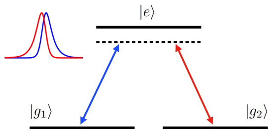
Figure 1. STIRAP scheme: two lower states $\left|g_1\right.⟩$ and $\left|g_2\right.⟩$ are coupled to an upper state $\left|e\right.⟩$ through suitable pulses. The dashed line represents a ‘virtual level’ of energy ${\nu }^{\prime }$. The inset shows the typical shape of the pulses.

Introducing the Hermitian operator, $G_1={\nu }^{\prime }\left|e\right.⟩\left.⟨e\right|+H_B$, and the relevant unitary operator $U_1$, such that $\mathrm{i}{\dot{U}}_1=G_1{U}_1$, in the new picture given by $|\tilde{\psi }\left(t\right)⟩=U_1^{†}\left(t\right)\left|\psi \left(t\right)\right.⟩$ and $\tilde{A}\left(t\right)=U_1^{†}\left(t\right)A\left(t\right)U_1\left(t\right)$ one finds that the generator of the time evolution is:

$$\tilde{H}\left(t\right)-G_1=H_A^{\prime }+{\tilde{H}}_S^{\left(0\right)}\left(t\right)+{\tilde{H}}_S^{\left(\omega \right)}\left(t\right)+{\tilde{H}}_{AB}\left(t\right),$$

(6)

with

$$\begin{array}{c}\hfill H_A^{\prime }=(\nu -{\nu }^{\prime })\left|e\right.⟩\left.⟨e\right|,\end{array}$$

(7)

$$\begin{array}{ccc}\hfill {\tilde{H}}_S^{\left(0\right)}\left(t\right)& =& \sum _{m=1}^2{\mathrm{\Omega }}_m\left(t\right)(\left|g_m\right.⟩\left.⟨e\right|+\left|e\right.⟩\left.⟨g_m\right|),\hfill \end{array}$$

(8)

$$\begin{array}{ccc}\hfill {\tilde{H}}_S^{\left(\omega \right)}\left(t\right)& =& \sum _{m=1}^2{\mathrm{\Omega }}_m\left(t\right)\left|g_m\right.⟩\left.⟨e\right|{\mathrm{e}}^{-\mathrm{i}2{\nu }^{\prime }t}+\mathrm{h}.\mathrm{c}.,\hfill \end{array}$$

(9)

$$\begin{array}{ccc}\hfill {\tilde{H}}_{AB}\left(t\right)& =& \sum _{m=1}^2(\left|g_m\right.⟩\left.⟨e\right|{\mathrm{e}}^{-\mathrm{i}{\nu }^{\prime }t}+\left|e\right.⟩\left.⟨g_m\right|{\mathrm{e}}^{\mathrm{i}{\nu }^{\prime }t})\otimes \sum _k{\eta }_k^{\left(m\right)}({\sigma }_{-}^{\left(k\right)}{\mathrm{e}}^{-\mathrm{i}\omega t}+{\sigma }_{+}^{\left(k\right)}{\mathrm{e}}^{\mathrm{i}\omega t}),\hfill \end{array}$$

(10)

with ⊗ denoting the tensor product, “h.c.” standing for the “Hermitian conjugate” term, $\Delta =\nu -{\nu }^{\prime }$ being the detuning between the atomic frequency and the field frequency. It is worth mentioning that, in view of the further treatments, we have split the transformed pulse Hamiltonian ${\tilde{H}}_S$ into two contributions, ${\tilde{H}}_S={\tilde{H}}_S^{\left(0\right)}+{\tilde{H}}_S^{\left(\omega \right)}$, where the first corresponds to the so called rotating terms (characterized by the absence of fast oscillations) while the second is related to the counter-rotating terms (rapidly oscillating). For our treatment of the system–bath interaction terms in ${\tilde{H}}_{AB}\left(t\right)$, this separation of rotating and counter-rotating terms is not necessary.

2.2. Ideal STIRAP

Let us first sum up the basic form of the ideal STIRAP, which corresponds to the absence of interaction with the environment (referring to our model, this condition is accomplished assuming ${\eta }_k^{\left(m\right)}=0$, $\forall m,k$). Moreover, assuming high atomic and field frequencies, one is legitimated to neglect the counter-rotating terms in the STIRAP Hamiltonian, so that the system can be assumed to be approximately ruled only by $H_A^{\prime }+{\tilde{H}}_S^{\left(0\right)}$ in this new picture usually, which is referred to as the rotating frame. The operator

$$\begin{array}{c}\hfill H_A^{\prime }+{\tilde{H}}_S^{\left(0\right)}\left(t\right)=\Delta \left|e\right.⟩\left.⟨e\right|+\sum _{m=1}^2{\mathrm{\Omega }}_m\left(t\right)(\left|g_m\right.⟩\left.⟨e\right|+\left|e\right.⟩\left.⟨g_m\right|),\end{array}$$

(11)

can be diagonalized at every instant of time, and its instantaneous eigenstates are:

$$\begin{array}{ccc}\hfill \left|+\left(t\right)\right.⟩& =& sin\phi \left(t\right)sin\theta \left(t\right)\left|g_1\right.⟩+cos\phi \left(t\right)\left|e\right.⟩+sin\phi \left(t\right)cos\theta \left(t\right)\left|g_2\right.⟩,\hfill \end{array}$$

(12)

$$\begin{array}{ccc}\hfill \left|0\left(t\right)\right.⟩& =& cos\theta \left(t\right)\left|g_1\right.⟩-sin\theta \left(t\right)\left|g_2\right.⟩,\hfill \end{array}$$

(13)

$$\begin{array}{ccc}\hfill \left|-\left(t\right)\right.⟩& =& cos\phi \left(t\right)sin\theta \left(t\right)\left|g_1\right.⟩-sin\phi \left(t\right)\left|e\right.⟩+cos\phi \left(t\right)cos\theta \left(t\right)\left|g_2\right.⟩,\hfill \end{array}$$

(14)

where

$$\begin{array}{cc}\hfill tan\theta \left(t\right)& =\frac{{\mathrm{\Omega }}_1\left(t\right)}{{\mathrm{\Omega }}_2\left(t\right)},\hfill \end{array}$$

(15)

$$\begin{array}{cc}\hfill tan2\phi \left(t\right)& =\frac{2{\mathrm{\Omega }}_L\left(t\right)}{\Delta },\hfill \end{array}$$

(16)

$$\begin{array}{cc}\hfill {\mathrm{\Omega }}_L\left(t\right)& =\sqrt{{\mathrm{\Omega }}_1^2\left(t\right)+{\mathrm{\Omega }}_2^2\left(t\right)}.\hfill \end{array}$$

(17)

Such eigenstates correspond to the following eigenvalues:

$$\begin{array}{c}\hfill E_0=0,E_{\pm }=\frac{1}{2}\left[\Delta \pm \sqrt{{\Delta }^2+4{\mathrm{\Omega }}_L^2\left(t\right)}\right]\end{array}$$

(18)

The standard STIRAP process aimed at transferring population from the state $\left|g_1\right.⟩$ to $\left|g_2\right.⟩$ is realized through a so-called counterintuitive sequence, where the pulse ${\mathrm{\Omega }}_2$ precedes ${\mathrm{\Omega }}_1$. Accordingly, at the initial time $\theta =0$ and $\phi =0$, so that $\left|+\right.⟩=\left|e\right.⟩$, $\left|0\right.⟩=\left|g_1\right.⟩$ and $\left|-\right.⟩=\left|g_2\right.⟩$, while in the final time $\theta =\pi /2$ and $\phi =0$, so that $\left|+\right.⟩=\left|e\right.⟩$, $\left|0\right.⟩=-\left|g_2\right.⟩$ and $\left|-\right.⟩=\left|g_1\right.⟩$. When the pulse profiles are slowly varying functions, the hypotheses of the adiabatic theorem are satisfied and the population of each eigenstate is preserved during the evolution. Consequently, in particular, the population of the state $\left|g_1\right.⟩$, initially coinciding with $\left|0\right.⟩$, is totally transferred to the state $\left|g_2\right.⟩$, which equals $\left|0\right.⟩$ in the final time.

2.3. Time Evolution and Efficiency

In order to better evaluate the effects of the remaining terms of the Hamiltonian, we perform a new change of picture, applying the transformation $\left|\overline{\psi }\right.⟩=U_2^{†}\left|\tilde{\psi }\right.⟩$ with $U_2$ such that $\mathrm{i}{\dot{U}}_2=(H_A^{\prime }+{\tilde{H}}_S^{\left(0\right)}\left(t\right))U_2$.

The operator $U_2$ is well approximated by the unitary evolution describing the adiabatic following of the instantaneous eigenstates of the Hamiltonian $H_A^{\prime }+{\tilde{H}}_S^{\left(0\right)}\left(t\right)$, given by $U_2(t,t_0)\approx {\sum }_m{\mathrm{e}}^{-\mathrm{i}{\alpha }_m(t,t_0)}\left|{\varphi }_m\left(t\right)\right.⟩\left.⟨{\varphi }_m\left(t_0\right)\right|$, with $\left|{\varphi }_m\left(t\right)\right.⟩$ being the instantaneous eigenstates of $H_A^{\prime }+{\tilde{H}}_S^{\left(0\right)}\left(t\right)$, and ${\alpha }_m(t,t_0)={\int }_{t_0}^t{E}_m\left(w\right)\mathrm{d}w+$ $\mathrm{i}{\int }_{t_0}^t\left({\partial }_w\left.⟨{\varphi }_m\left(w\right)\right|\right)\left|{\varphi }_m\left(w\right)\right.⟩\mathrm{d}w$ being the relevant phase factors. It is worth mentioning that all the geometric phases are zero, which comes from the feature that $\left({\partial }_w\left.⟨{\varphi }_m\left(w\right)\right|\right)\left|{\varphi }_m\left(w\right)\right.⟩$, with ${\partial }_w\equiv \partial /\partial w$, is always an imaginary number, while the coefficients of the eigenstates are all real, which implies that all such terms are zero. Applying the transformation, one obtains:

$$\overline{H}\left(t\right)-{\overline{G}}_2\left(t\right)={\overline{H}}_S^{\left(\omega \right)}\left(t\right)+{\overline{H}}_{AB}\left(t\right),$$

(19)

with

$$\begin{array}{ccc}\hfill {\overline{H}}_S^{\left(\omega \right)}\left(t\right)& =& \sum _{m=1}^2{\mathrm{\Omega }}_m\left(t\right)\left|{\mathring{g}}_m\left(t\right)\right.⟩\left.⟨\mathring{e}\left(t\right)\right|{\mathrm{e}}^{-\mathrm{i}2{\nu }^{\prime }t}+h.c.,\hfill \end{array}$$

(20)

$$\begin{array}{ccc}\hfill {\overline{H}}_{AB}\left(t\right)& =& \sum _{m=1}^2(\left|{\mathring{g}}_m\left(t\right)\right.⟩\left.⟨\mathring{e}\left(t\right)\right|{\mathrm{e}}^{-\mathrm{i}{\nu }^{\prime }t}+\left|\mathring{e}\left(t\right)\right.⟩\left.⟨{\mathring{g}}_m\left(t\right)\right|{\mathrm{e}}^{\mathrm{i}{\nu }^{\prime }t})\hfill \\ & \otimes & \sum _k{\eta }_k^{\left(m\right)}({\sigma }_{-}^{\left(k\right)}{\mathrm{e}}^{-\mathrm{i}\omega t}+{\sigma }_{+}^{\left(k\right)}{\mathrm{e}}^{\mathrm{i}\omega t}),\hfill \end{array}$$

(21)

with $\left|{\mathring{g}}_m\left(t\right)\right.⟩=U_2^{†}(t,t_0)\left|g_m\right.⟩$ and $\left|\mathring{e}\left(t\right)\right.⟩=U_2^{†}(t,t_0)\left|e\right.⟩$.

In the new picture, the generator of the time evolution is the following:

$$\begin{array}{c}\hfill {\overline{H}}_G={\overline{H}}_S^{\left(\omega \right)}\left(t\right)+{\overline{H}}_{AB}\left(t\right),\end{array}$$

(22)

and the relevant approximated dynamics can be evaluated, to the second order, by truncation of the iterated formal solution:

$$\begin{array}{c}\hfill T(t,t_0)\approx 11-\mathrm{i}{\int }_{t_0}^t{\overline{H}}_G\left(w\right)\mathrm{d}w-{\int }_{t_0}^t\mathrm{d}w{\int }_{t_0}^w\mathrm{d}{w}^{\prime }{\overline{H}}_G\left(w\right){\overline{H}}_G\left(w^{\prime }\right)\equiv T_2(t,t_0),\end{array}$$

(23)

which is essentially the truncation of the Dyson series (expressed without the chronological ordering operator) to the second order.

Moreover, since we have moved to this new picture by removing the adiabatic evolution operator responsible for a perfect population transfer from $\left|g_1\right.⟩$ to $\left|g_2\right.⟩$, remaining in the state $\left|g_1\right.⟩$ is equivalent to undergoing a perfect transition from $\left|g_1\right.⟩$ to $\left|g_2\right.⟩$ in the Schrödinger picture. Therefore, in the new picture the efficiency of the population transfer process through STIRAP pulses is given by the survival probability of the initial state of the three-state system:

$$\begin{array}{c}\hfill P\left(t\right)=\mathrm{tr}[T(t,t_0)\left|\psi \left(0\right)\right.⟩\left.⟨\psi \left(0\right)\right|{\rho }_B\left(0\right)T^{†}\left(t\right)\left|\psi \left(0\right)\right.⟩\left.⟨\psi \left(0\right)\right|\otimes 11_B],\end{array}$$

(24)

where ${\rho }_B\left(0\right)$ is the density operator describing the initial configuration of the bath, $11_B$ is the identity operator of the bath and $T(t,t_0)$ is possibly replaced by $T_2(t,t_0)$ and “tr” stands for the trace operation. In the case considered here, $\left|\psi \left(0\right)\right.⟩=\left|g_1\right.⟩$. In order to better understand Equation (24), consider that the complete time evolution of the initial state $\left|g_1\right.⟩\left.⟨g_1\right|\otimes {\rho }_B\left(0\right)$ in the Schrödinger picture is given by: ${\rho }_{AB}\left(t\right)={\mathcal{U}}_1(t,t_0){\mathcal{U}}_2(t,t_0)T(t,t_0)\left|g_1\right.⟩\left.⟨g_1\right|\otimes {\rho }_B\left(0\right)T^{†}(t,t_0){\mathcal{U}}_2^{†}(t,t_0){\mathcal{U}}_1^{†}(t,t_0)$. Now, since the target state is $\left|g_2\right.⟩$, irrespective of the state of the bath, we need to evaluate $P\left(t\right)=\mathrm{tr}[{\rho }_{AB}\left(t\right)$$\left|g_2\right.⟩\left.⟨g_2\right|\otimes 11_B]$, which, after performing two cyclic permutations inside the trace functional leads to the following expression: $\mathrm{tr}[T(t,t_0)\left|g_1\right.⟩\left.⟨g_1\right|{\rho }_B\left(0\right)T^{†}(t,t_0){\mathcal{U}}_2^{†}(t,t_0){\mathcal{U}}_1^{†}(t,t_0)\left|g_2\right.⟩\left.⟨g_2\right|\otimes 11_B{\mathcal{U}}_2(t,t_0)$${\mathcal{U}}_1(t,t_0)]$, which is equivalent to Equation (24) once it is considered that ${\mathcal{U}}_2(t,t_0)\left|g_1\right.⟩=\left|g_2\right.⟩$, and conversely, ${\mathcal{U}}_2^{†}(t,t_0)\left|g_2\right.⟩=\left|g_1\right.⟩$, so that ${\mathcal{U}}_2^{†}(t,t_0){\mathcal{U}}_1^{†}(t,t_0)\left|g_2\right.⟩\left.⟨g_2\right|\otimes 11_B{\mathcal{U}}_1(t,t_0){\mathcal{U}}_2(t,t_0)=$$\left|g_1\right.⟩\left.⟨g_1\right|\otimes 11_B$.

3. Results

We now focus on the zero-temperature bath, which means assuming that the spin bath is initially in its ground state: $\left|\{\downarrow \}\right.⟩={\otimes }_k{\left|\downarrow \right.⟩}_k$. Therefore, the complete initial state is $\left|g_1\right.⟩\left|\{\downarrow \}\right.⟩$. Since we are considering the approximation $T(t,t_0)\approx T_2(t,t_0)$ according to Equation (23), the only transitions considered in our calculations are those involving zero, one or two spin flips in the bath. This implies the following form for the efficiency:

$$\begin{array}{ccc}\hfill P\left(t\right)& \approx & |\left.⟨\{\downarrow \}\right|\left.⟨g_1\right|T_2(t,t_0)\left|g_1\right.⟩\left|\{\downarrow \}\right.⟩{|}^2\hfill \\ \hfill & +& {\mathrm{\Sigma }}_l{\left|\left.⟨{\{\downarrow \}\uparrow }_l\{\downarrow \}\right|\left.⟨g_1\right|T_2(t,t_0)\left|g_1\right.⟩\left|\{\downarrow \}\right.⟩\right|}^2\hfill \\ & +& {\mathrm{\Sigma }}_{j\ne l}{\left|\left.⟨{\{\downarrow \}\uparrow }_j{\{\downarrow \}\uparrow }_l\{\downarrow \}\right|\left.⟨g_1\right|T_2(t,t_0)\left|g_1\right.⟩\left|\{\downarrow \}\right.⟩\right|}^2,\hfill \end{array}$$

(25)

where $\left|{\{\downarrow \}\uparrow }_l\{\downarrow \}\right.⟩$ is the bath state with all spins in the $\left|\downarrow \right.⟩$ state, except for the l-th spin, which is the $\left|\uparrow \right.⟩$ state, while $\left|{\{\downarrow \}\uparrow }_j{\{\downarrow \}\uparrow }_l\{\downarrow \}\right.⟩$ has only the l-th and j-th spins in the $\left|\uparrow \right.⟩$ state, all the others being in the state $\left|\downarrow \right.⟩$. The overlaps involving only one spin flip turn out to be zero (see Appendix B for details). The overlaps involving two spin flips involve only second-order terms and, once their squared modulus is evaluated, such terms give rise to fourth-order contributions. To make the calculation consistent with the truncation of the Dyson series to the second order, only terms up to the second order are to be kept in the probability, which gives the following expression:

$$\begin{array}{c}\hfill P\left(t\right)\approx 1-2\Re \left[{\mathcal{J}}_{\left\{{\eta }_k^{\left(m\right)}\right\}}\left(t\right)\right],\end{array}$$

(26)

where ℜ denotes the real part, and its argument is the following integral:

$$\begin{array}{ccc}\hfill {\mathcal{J}}_{\left\{{\eta }_k^{\left(m\right)}\right\}}\left(t\right)& =& {\int }_{t_0}^t\mathrm{d}w{\int }_{t_0}^w\mathrm{d}{w}^{\prime }[{\mathrm{e}}^{-\mathrm{i}{\int }_w^{w^{\prime }}{E}_{+}\left(s\right)\mathrm{d}s}cos\phi \left(w\right)cos\phi \left(w^{\prime }\right)\hfill \\ \hfill & +& {\mathrm{e}}^{-\mathrm{i}{\int }_w^{w^{\prime }}{E}_{-}\left(s\right)\mathrm{d}s}sin\phi \left(w\right)sin\phi \left(w^{\prime }\right)]{\mathrm{e}}^{\mathrm{i}({\nu }^{\prime }+\omega )(w^{\prime }-w)}\hfill \\ & \times & \sum _k\left[{\eta }_k^{\left(1\right)}cos\theta \left(w\right)-{\eta }_k^{\left(2\right)}sin\theta \left(w\right)\right]\left[{\eta }_k^{\left(1\right)}cos\theta \left(w^{\prime }\right)-{\eta }_k^{\left(2\right)}sin\theta \left(w^{\prime }\right)\right].\hfill \end{array}$$

(27)

We now assume that the quantities ${\eta }_k^{\left(m\right)}$, first defined after Equation (5) without any constraint, are related in such a way that the ratios ${\eta }_k^{\left(m\right)}/{\eta }_1^{\left(m\right)}$ do not depend on m, so that one can introduce ${\lambda }_k\equiv {\eta }_k^{\left(m\right)}/{\eta }_1^{\left(m\right)}$, define the following quantities:

$$\begin{array}{c}\hfill \eta \equiv {\eta }_1^{\left(1\right)},r_{\eta }\equiv {\eta }_1^{\left(2\right)}/{\eta }_1^{\left(1\right)},\mathrm{\Lambda }\equiv \sum _k{\lambda }_k^2,\end{array}$$

(28)

and recast the probability in the following form:

$$\begin{array}{c}\hfill P\left(t\right)\approx 1-2{\eta }^2\mathrm{\Lambda }\Re \left[\mathcal{J}\left(t\right)\right],\end{array}$$

(29)

with

$$\begin{array}{ccc}\hfill \mathcal{J}\left(t\right)& =& {\int }_{t_0}^t\mathrm{d}w{\int }_{t_0}^w\mathrm{d}{w}^{\prime }\left[{\mathrm{e}}^{-\mathrm{i}{\int }_w^{w^{\prime }}{E}_{+}\left(s\right)\mathrm{d}s}cos\phi \left(w\right)cos\phi \left(w\right)+{\mathrm{e}}^{-\mathrm{i}{\int }_w^{w^{\prime }}{E}_{-}\left(s\right)\mathrm{d}s}sin\phi \left(w\right)sin\phi \left(w^{\prime }\right)\right]\hfill \\ & \times & {\mathrm{e}}^{\mathrm{i}({\nu }^{\prime }+\omega )(w^{\prime }-w)}\left[cos\theta \left(w\right)-r_{\eta }sin\theta \left(w\right)\right]\left[cos\theta \left(w^{\prime }\right)-r_{\eta }sin\theta \left(w^{\prime }\right)\right].\hfill \end{array}$$

(30)

On the basis of Equation (29), the survival probability of the initial state in the interaction picture, which corresponds to the efficiency of the population transfer in the Schrödinger picture, turns out to differ from unity by a term proportional to the real part of the the integral $\mathcal{J}\left(t\right)$ (having the dimensions of the square of time), on which we focus in what follows. Every specific correction should take into account the specific value of the square of the quantity $\eta \sqrt{\mathrm{\Lambda }}$ (having the dimension of a frequency), which somehow is a cumulative measure of the coupling strength between the three-level system and the whole environment. It is also interesting to observe that, in the RWA, the counterpart of $\mathcal{J}\left(t\right)$ would be zero. This can be straightforwardly proven by recalculating the relevant matrix elements. Moreover, it is already clearly visible from the expression of $\mathcal{J}\left(t\right)$, where all the terms contain rapidly oscillating factors coming from the fact that all the contributions come out as matrix elements of the counter-rotating terms.

It is worth mentioning that the assumption ${\eta }_k^{\left(m\right)}/{\eta }_1^{\left(m\right)}$, independent from the index m, is not as restrictive as one could think, since the coupling strengths are supposed to be proportional to a function of the spin distance from the central three-state system, and this proportionality function is supposed to be the same independently of the specific transitions involved, whether $\left|e\right.⟩\leftrightarrow \left|g_1\right.⟩$ or $\left|e\right.⟩\leftrightarrow \left|g_2\right.⟩$. Concerning the shape of the pulses, they are usually taken as Gaussian, with the peaks occurring at different times. In particular, we assume two pulses centered at $\pm \tau$ and with a width $\tau /\sqrt{2}$:

$$\begin{array}{c}\hfill {\mathrm{\Omega }}_1={\mathrm{\Omega }}_0{\mathrm{e}}^{-{(t/\tau +1)}^2},\end{array}$$

(31)

$$\begin{array}{c}\hfill {\mathrm{\Omega }}_1={\mathrm{\Omega }}_0{\mathrm{e}}^{-{(t/\tau -1)}^2}.\end{array}$$

(32)

The process is supposed to start at time $t_0=-T$ (with $T>\tau$) and finish at $t=T$. In Figure 2 and Figure 3 the numerically calculated quantity $2\Re \left\{\mathcal{J}\right(T\left)\right\}$ is reported as a function of different parameters, which allows us to evaluate the efficiency of the population transfer in several regimes: the smaller the quantity $2\Re \left\{\mathcal{J}\right(T\left)\right\}$, the more efficient the population transfer, according to Equation (29). In all the plots we have assumed that the parameters of the pulses satisfy the following conditions, which guarantee an optimal transfer in the ideal case: ${\mathrm{\Omega }}_0\tau =10$, $T/\tau =5$, $\nu \tau =10$.

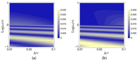
Figure 2. The quantity $2\Re \left\{\mathcal{J}\right(T\left)\right\}$ (in units of ${\tau }^2$) as a function of $\omega$ (in units of $\nu$ and logarithmic scale) and $\Delta$ (in units of $\nu$) in the case $r_{\eta }=1$ (a) and $r_{\eta }=-1$ (b). The other parameters are: ${\mathrm{\Omega }}_0\tau =10$, $T/\tau =5$, $\nu \tau =10$. See text for details.

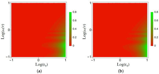
Figure 3. The quantity $2\Re \left\{\mathcal{J}\right(T\left)\right\}$ (in units of ${\tau }^2$) as a function of $\omega$ (in units of $\nu$ and logarithmic scale) and $r_{\eta }$ (in logarithmic scale) for $\Delta =0.01\nu$ (a) and $\Delta =0.05\nu$ (b). The other parameters are: ${\mathrm{\Omega }}_0\tau =10$, $T/\tau =5$, $\nu \tau =10$. See text for details.

In Figure 2, $2\Re \left\{\mathcal{J}\right(T\left)\right\}$ is shown as a function of $\omega$ and $\Delta$ for two values of the ratio $r_{\eta }$, in particular, for $r_{\eta }=1$ (Figure 2a) and $r_{\eta }=-1$ (Figure 2b). In both plots it is clearly visible that the value of $2\Re \left\{\mathcal{J}\right(T\left)\right\}$ is always small, never exceeding the value $0.03$, and that, for high values of the frequency $\omega$, the corrections become smaller and smaller. For any fixed value of $\Delta$, one can see that, when varying the value of $\omega$, the quantity $2\Re \left\{\mathcal{J}\right(T\left)\right\}$ exhibits an oscillatory behavior, which a posteriori can be related to the presence of the phase factor $exp\left[(\omega +{\nu }^{\prime })(w^{\prime }-w)\right]$ in the integrand. Actually, in spite of the presence of other functions, the mentioned phase factor is indeed the main rapidly changing factor, whereas trigonometric functions of $\varphi$ and $\theta$ are smoothly changing and the phase factor associated with the integral of $E_{+}$ changes rapidly only in the region between the two peaks. Thus, both the presence of oscillations and the vanishing of $\mathcal{J}\left(T\right)$ for higher values of $\nu$ are traceable back to the oscillatory character of the counter-rotating terms. By comparing Figure 2a and Figure 2b, it emerges that, whether the value of the ratio parameter $r_{\eta }$ is 1 or $-1$, the behavior is quite similar, though significant differences are present, particularly in the region corresponding to small values of $\Delta$.

In Figure 3, $2\Re \left\{\mathcal{J}\right(T\left)\right\}$ is shown as a function of $\omega$ and $r_{\eta }$ for two values of the detuning $\Delta$, in particular, for $\Delta /\nu =0.01$ (Figure 3a) and $\Delta /\nu =0.05$ (Figure 3b). One can see that the values of the quantity in a particular parameter region are much higher than in Figure 2, reaching the value of $0.8$. These high values can be justified by the fact that increasing the value of $r_{\eta }$ implies increasing the amplitude of the coupling term between the three-state system and the environment. In particular, a high value of $r_{\eta }$ means dealing with a high value of ${\eta }_1^{\left(2\right)}$ (and consequently all ${\eta }_k^{\left(2\right)}$), which in turn implies a higher value of $\mathcal{J}\left(T\right)$.

In order to fix the ideas about the meaning of our results, let us consider the case where $\eta \sqrt{\mathrm{\Lambda }}\tau =1$ means $\eta \sqrt{\mathrm{\Lambda }}/{\mathrm{\Omega }}_0\ll 1$, thus the perturbation treatment is kept valid. In such a case, in the greener region of Figure 3, the correction would be about $0.8$, implying a quite low efficiency, of about $0.2$. On the contrary, in the most problematic region of Figure 2, consisting of the yellow parts corresponding to values close to $0.03$, the efficiency would be about $0.97$.

4. Discussion

In this paper, we have considered the effects of the interaction with a spin bath on the efficiency of a population transfer realized through a STIRAP process. Our present study is an evolution of the earlier studyreported in ref. [56], where the system–bath interaction has been considered in the RWA. Here, in order to improve the analysis, we have also considered the effects of the counter-rotating terms. Nevertheless, since the model analyzed is not exactly solvable and its numerical treatment would be challenging, we have faced the problem through a perturbation approach. In particular, second order corrections have been calculated by evaluating the Dyson series truncated to the second order contributions. The complete deviation of the efficiency of the population transfer from unity, according to Equation (29), turns out to be proportional to the square of $\eta \sqrt{\mathrm{\Lambda }}$, which plays the role of a perturbation parameter. It is important to note that $\eta \sqrt{\mathrm{\Lambda }}=\sqrt{{\sum }_k{\left({\eta }_k^{\left(1\right)}\right)}^2}$ and $r_{\eta }\eta \sqrt{\mathrm{\Lambda }}=\sqrt{{\sum }_k{\left({\eta }_k^{\left(2\right)}\right)}^2}$, which correspond to the effective strengths of the couplings with the environment involving $\left|g_1\right.⟩\leftrightarrow \left|e\right.⟩$ transitions and $\left|g_2\right.⟩\leftrightarrow \left|e\right.⟩$ transitions, respectively. Beyond this fact, according to Equation (29), the correction to the efficiency of population transfer is proportional to the real part of the integral $\mathcal{J}\left(T\right)$ defined in Equation (30).

Remarkably, in a second order perturbation treatment under the RWA, the correction to the efficiency would be zero, thus predicting a perfect population transfer. On the contrary, beyond such an approximation, deviations come up. As a matter of fact, our analysis shows that, in the second perturbation treatment, the counter-rotating terms in the interaction are the only ones really contributing to the corrections. Indeed, in the integrand of $\mathcal{J}\left(T\right)$ only contributions proportional to the phase factor $exp\left[(\omega +{\nu }^{\prime })(w^{\prime }-w)\right]$ appear to be traceable back the rapidly oscillating terms in the interaction (namely, the counter-rotating terms), while no term proportional to a phase factor associated with a lower frequency $\omega -{\nu }^{\prime }$ (the rotating terms) is present. This implies that, in a model involving RWA, the correction is zero, which is perfectly in agreement with the results of ref. [56] where the efficiency always exhibits a plateau in the weak coupling limit and up to the weak–intermediate coupling regime.

The numerical evaluation of the integral $\mathcal{J}\left(T\right)$ reported in Figure 2 and Figure 3 shows that, in the range of the parameters analyzed the effects of the environment are mainly negligible, except for specific regions where the ratio $r_{\eta }$ assumes high values, since this implies that the coupling constants ${\eta }_k^{\left(2\right)}$ are significant. Further numerical results (not reported in this paper because they would essentially provide uniform functions corresponding to zero values) show in a clear way that higher and higher values of $\nu$ imply smaller and smaller corrections, due to the fact that counter-rotating terms become more and more rapidly oscillating and thus ineffective. Summing up, negligibility of the effects of the environment is obtained for high values of $\omega$ (according to the plates shown in the paper) or high values of $\nu$ (according to other simulations), provided $r_{\eta }$ is not exceptionally large. Naturally, the values of $\eta \sqrt{\mathrm{\Lambda }}$ are to be kept small enough to maintain the validity of our analysis based on perturbation theory.

It is worth concluding with two more comments concerning a comparison with the results reported in ref. [56]. First, since our second-order perturbation treatment is valid only in the weak coupling regime, we cannot obtain corrections in the strong coupling regime where a generalized quantum Zeno effect were predicted to occur. Second, the shape of the pulses considered here is properly Gaussian, while in ref. [56], different expressions have been considered. Nevertheless, in spite of the more complicated analytical expression, the pulses in ref. [56] are essentially Gaussian too, in the sense that they only slightly differ form the Gaussian counterparts, which makes the two situations comparable.

References

- Messiah, A. Quantum Mechanics; Dover Publications, Inc.: Mineola, NY, USA, 1999; Available online: https://archive.org/details/quantummechanics0000mess/ (accessed on 2 February 2024).
- Griffiths, D.J.; Schroeter, D.F. Introduction to Quantum Mechanics; Cambridge University Press: New York, NY, USA, 2018. [Google Scholar] [CrossRef]
- Albash, T.; Lidar, D.A. Adiabatic quantum computation. Rev. Mod. Phys. 2018, 90, 015002. [Google Scholar] [CrossRef]
- Santos, A.C.; Sarandy, M.S. Sufficient conditions for adiabaticity in open quantum systems. Phys. Rev. A 2020, 102, 052215. [Google Scholar] [CrossRef]
- Il’in, N.; Aristova, A.; Lychkovskiy, O. Adiabatic theorem for closed quantum systems initialized at finite temperature. Phys. Rev. A 2021, 104, L030202. [Google Scholar] [CrossRef]
- Pyshkin, P.V.; Luo, D.W.; Wu, L.A. Self-protected adiabatic quantum computation. Phys. Rev. A 2022, 106, 012420. [Google Scholar] [CrossRef]
- Coello Pérez, E.A.; Bonitati, J.; Lee, D.; Quaglioni, S.; Wendt, K.A. Quantum state preparation by adiabatic evolution with custom gates. Phys. Rev. A 2022, 105, 032403. [Google Scholar] [CrossRef]
- Vitanov, N.V.; Fleischhauer, M.; Shore, B.W.; Bergmann, K. Coherent manipulation of atoms molecules by sequential laser pulses. Adv. At. Mol. Opt. Phys. 2001, 46, 55–190. [Google Scholar] [CrossRef]
- Vitanov, N.V.; Halfmann, T.; Shore, B.W.; Bergmann, K. Laser-induced population transfer by adiabatic passage. Ann. Rev. Phys. Chem. 2001, 52, 763–809. [Google Scholar] [CrossRef] [PubMed]
- Bergmann, K.; Theuer, H.; Shore, B.W. Coherent population transfer among quantum states of atoms and molecules. Rev. Mod. Phys. 1998, 70, 1003–1025. [Google Scholar] [CrossRef]
- Král, P.; Thanopulos, I.; Shapiro, M. Colloquium: Coherently controlled adiabatic passage. Rev. Mod. Phys. 2007, 79, 53–77. [Google Scholar] [CrossRef]
- Bergmann, K.; Nägerl, H.-C.; Panda, C.; Gabrielse, G.; Miloglyadov, E.; Quack, M.; Seyfang, G.; Wichmann, G.; Ospelkaus, S.; Kuhn, A.; et al. Roadmap on STIRAP applications. J. Phys. B At. Mol. Opt. Phys. 2019, 52, 202001. [Google Scholar] [CrossRef]
- Blekos, K.; Stefanatos, D.; Paspalakis, E. Performance of superadiabatic stimulated Raman adiabatic passage in the presence of dissipation and Ornstein-Uhlenbeck dephasing. Phys. Rev. A 2020, 102, 023715. [Google Scholar] [CrossRef]
- Ahmadinouri, F.; Hosseini, M.; Sarreshtedari, F. Stimulated Raman adiabatic passage: Effects of system parameters on population transfer. Chem. Phys. 2020, 539, 110960. [Google Scholar] [CrossRef]
- Cinins, A.; Bruvelis, M.; Bezuglov, N.N. Study of the adiabatic passage in tripod atomic systems in terms of the Riemannian geometry of the Bloch sphere. J. Phys. B At. Mol. Opt. Phys. 2022, 55, 234003. [Google Scholar] [CrossRef]
- Dogra, S.; Paraoanu, G.S. Perfect stimulated Raman adiabatic passage with imperfect finite-time pulses. J. Phys. B At. Mol. Opt. Phys. 2022, 55, 174001. [Google Scholar] [CrossRef]
- Liu, K.; Sugny, D.; Chen, X.; Guérin, S. Optimal pulse design for dissipative-stimulated Raman exact passage. Entropy 2023, 25, 790. [Google Scholar] [CrossRef] [PubMed]
- Genov, G.T.; Rochester, S.; Auzinsh, M.; Jelezko, F.; Budker, D. Robust two-state swap by stimulated Raman adiabatic passage. J. Phys. B At. Mol. Opt. Phys. 2023, 56, 054001. [Google Scholar] [CrossRef]
- Ni, K.-K.; Ospelkaus, S.; de Miranda, M.H.G.; Peér, A.; Neyenhuis, B.; Zirbel, J.J.; Kotochigova, S.; Julienne, P.S.; Jin, D.S.; Ye, J. A high phase-space-density gas of polar molecules. Science 2008, 322, 231–235. [Google Scholar] [CrossRef]
- Danzl, J.G.; Haller, E.; Gustavsson, M.; Mark, M.J.; Hart, R.; Bouloufa, N.; Dulieu, O.; Ritsch, H.; Nägerl, H.-C. Quantum Gas of deeply bound ground state molecules. Science 2008, 321, 1062–1066. [Google Scholar] [CrossRef] [PubMed]
- Danzl, J.G.; Mark, M.J.; Haller, E.; Gustavsson, M.; Hart, R.; Aldegunde, J.; Hutson, J.M.; Nägerl, H.-C. An ultracold high-density sample of rovibronic ground-state molecules in an optical lattice. Nat. Phys. 2010, 6, 265–270. [Google Scholar] [CrossRef]
- Klein, J.; Beil, F.; Halfmann, T. Robust Population transfer by stimulated Raman adiabatic passage in a Pr3+:Y2SiO5 Crystal. Phys. Rev. Lett. 2007, 99, 113003. [Google Scholar] [CrossRef] [PubMed]
- Alexander, A.L.; Lauro, R.; Louchet, A.; Chanelière, T.; Le Gouët, J.L. Stimulated Raman adiabatic passage in Tm3+:YAG. Phys. Rev. B 2008, 78, 144407. [Google Scholar] [CrossRef]
- Golter, D.A.; Wang, H. Optically driven Rabi oscillations and adiabatic passage of single electron spins in diamond. Phys. Rev. Lett. 2014, 112, 116403. [Google Scholar] [CrossRef]
- Yale, C.G.; Heremans, F.J.; Zhou, B.B.; Auer, A.; Burkard, G.; Awschalom, D.D. Optical manipulation of the Berry phase in a solid-state spin qubit. Nat. Photon. 2016, 10, 184–189. [Google Scholar] [CrossRef]
- Wolfowicz, G.; Heremans, F.J.; Anderson, C.P.; Kanai, S.; Seo, H.; Gali, A.; Galli, G.; Awschalom, D.D. Quantum guidelines for solid-state spin defects. Nat. Rev. Mater. 2021, 6, 906925. [Google Scholar] [CrossRef]
- Zhou, B.; Baksic, A.; Ribeiro, H.; Yale, C.G.; Heremans, F.J.; Jerger, P.C.; Auer, A.; Burkard, G.; Clerk, A.A.; Awschalom, D.D. Accelerated quantum control using superadiabatic dynamics in a solid-state lambda system. Nat. Phys. 2017, 13, 330–334. [Google Scholar] [CrossRef]
- Baksic, A.; Ribeiro, H.; Clerk, A.A. Speeding up adiabatic quantum state transfer by using dressed states. Phys. Rev. Lett. 2016, 116, 230503. [Google Scholar] [CrossRef]
- Varguet, H.; Rousseaux, B.; Dzsotjan, D.; Jauslin, H.R.; Guérin, S.; Colas des Francs, G. Dressed states of a quantum emitter strongly coupled to a metal nanoparticle. Opt. Lett. 2016, 41, 4480–4483. [Google Scholar] [CrossRef]
- Castellini, A.; Jauslin, H.R.; Rousseaux, B.; Dzsotjan, D.; Colas des Francs, G.; Messina, A.; Guérin, S. Quantum plasmonics with multi-emitters: Application to stimulated Raman adiabatic passage. Eur. Phys. J. D 2018, 72, 223. [Google Scholar] [CrossRef]
- Kubo, Y. Turn to the dark side. Nat. Phys. 2016, 12, 21–22. [Google Scholar] [CrossRef]
- Xu, H.K.; Song, C.; Liu, W.Y.; Xue, G.M.; Su, F.F.; Deng, H.; Tian, Y.; Zheng, D.N.; Han, S.; Zhong, Y.P.; et al. Coherent population transfer between uncoupled or weakly coupled states in ladder-type superconducting qutrits. Nat. Commun. 2016, 7, 11018. [Google Scholar] [CrossRef] [PubMed]
- Kumar, K.S.; Vepsäläinen, A.; Danilin, S.; Paraoanu, G.S. Stimulated Raman adiabatic passage in a three-level superconducting circuit. Nat. Commun. 2016, 7, 10628. [Google Scholar] [CrossRef] [PubMed]
- Soresen, J.L.; Moller, D.; Iversen, T.; Thomsen, J.B.; Jensen, F.; Staanum, P.; Voigt, D.; Drewsen, M. Efficient coherent internal state transfer in trapped ions using stimulated Raman adiabatic passage. New J. Phys. 2006, 8, 261. [Google Scholar] [CrossRef]
- Higgins, G.; Pokorny, F.; Zhang, C.; Bodart, Q.; Hennrich, M. Coherent control of a single trapped Rydberg ion. Phys. Rev. Lett. 2017, 119, 220501. [Google Scholar] [CrossRef]
- Fedoseev, V.; Luna, F.; Hedgepeth, I.; Löffler, W.; Bouwmeester, D. Stimulated Raman adiabatic passage in optomechanics. Phys. Rev. Lett. 2021, 126, 113601. [Google Scholar] [CrossRef]
- Guéry-Odelin, D.; Ruschhaupt, A.; Kiely, A.; Torrontegui, E.; Martínez-Garaot, S.; Muga, J.G. Shortcuts to adiabaticity: Concepts, methods, and applications. Rev. Mod. Phys. 2019, 91, 045001. [Google Scholar] [CrossRef]
- Vitanov, N.V. High-fidelity multistate stimulated Raman adiabatic passage assisted by shortcut fields. Phys. Rev. A 2020, 102, 023515. [Google Scholar] [CrossRef]
- Evangelakos, V.; Paspalakis, E.; Stefanatos, D. Optimal STIRAP shortcuts using the spin-to-spring mapping. Phys. Rev. A 2023, 107, 052606. [Google Scholar] [CrossRef]
- Stefanatos, D.; Paspalakis, E. Optimal shortcuts of stimulated Raman adiabatic passage in the presence of dissipation. Philos. Trans. R. Soc. Math. Phys. Eng. Sci. 2022, 380, 20210283. [Google Scholar] [CrossRef] [PubMed]
- Messikh, C.; Messikh, A. Robust stimulated Raman shortcuts to adiabatic passage with deep learning. EPL (Europhys. Lett.) 2022, 140, 48003. [Google Scholar] [CrossRef]
- Stefanatos, D.; Blekos, K.; Paspalakis, E. Robustness of STIRAP shortcuts under Ornstein-Uhlenbeck noise in the energy levels. Appl. Sci. 2020, 10, 1580. [Google Scholar] [CrossRef]
- Genov, G.T.; Vitanov, N.V. Dynamical suppression of unwanted transitions in multistate quantum systems. Phys. Rev. Lett. 2013, 110, 133002. [Google Scholar] [CrossRef] [PubMed]
- Yatsenko, L.P.; Shore, B.W.; Bergmann, K. Detrimental consequences of small rapid laser fluctuations on stimulated Raman adiabatic passage. Phys. Rev. A 2014, 89, 013831. [Google Scholar] [CrossRef]
- Vitanov, N.V.; Stenholm, S. Population transfer via a decaying state. Phys. Rev. A 1997, 56, 1463–1471. [Google Scholar] [CrossRef]
- Breuer, H.-P.; Petruccione, F. The Theory of Open Quantum Systems; Oxford University Press: Oxford, UK, 2002. [Google Scholar] [CrossRef]
- Gardiner, C.W.; Zoller, P. Quantum Noise: A Handbook of Markovian and Non-Markovian Quantum Stochastic Methods with Applications to Quantum Optics; Springer: Berlin/Heidelberg, Germany, 2004. [Google Scholar]
- Ivanov, P.A.; Vitanov, N.V.; Bergmann, K. Spontaneous emission in stimulated Raman adiabatic passage. Phys. Rev. A 2005, 72, 053412. [Google Scholar] [CrossRef]
- Akram, M.J.; Saif, F. Adiabatic population transfer based on a double stimulated Raman adiabatic passage. J. Russ. Laser Res. 2014, 35, 547–554. [Google Scholar] [CrossRef]
- Sukharev, M.; Malinovskaya, S.A. Stimulated Raman adiabatic passage as a route to achieving optical control in plasmonics. Phys. Rev. A 2012, 86, 043406. [Google Scholar] [CrossRef]
- Mathisen, T.; Larson, J. Liouvillian of the open STIRAP problem. Entropy 2018, 20, 20. [Google Scholar] [CrossRef]
- Davies, E.B.; Spohn, H. Open quantum systems with time-dependent Hamiltonians and their linear response. J. Stat. Phys. 1978, 19, 511–523. [Google Scholar] [CrossRef]
- Scala, M.; Militello, B.; Messina, A.; Vitanov, N.V. Stimulated Raman adiabatic passage in an open quantum system: Master equation approach. Phys. Rev. A 2010, 81, 053847. [Google Scholar] [CrossRef]
- Scala, M.; Militello, B.; Messina, A.; Vitanov, N.V. Stimulated Raman adiabatic passage in a Λ system in the presence of quantum noise. Phys. Rev. A 2011, 83, 012101. [Google Scholar] [CrossRef]
- Onizhuk, M.; Miao, K.C.; Blanton, J.P.; Ma, H.; Anderson, C.P.; Bourassa, A.; Awschalom, D.D.; Galli, G. Probing the Coherence of Solid-State Qubits at Avoided Crossings. Phys. Rev. X Quantum 2021, 2, 010311. [Google Scholar] [CrossRef]
- Militello, B.; Napoli, A. Adiabatic manipulation of a system interacting with a spin bath. Entropy 2023, 15, 2028. [Google Scholar] [CrossRef]
- Fischer, J.; Breuer, H.-P. Correlated projection operator approach to non-Markovian dynamics in spin baths. Phys. Rev. A 2007, 76, 052119. [Google Scholar] [CrossRef]
- Ferraro, E.; Breuer, H.-P.; Napoli, A.; Jivulescu, M.A.; Messina, A. Non-Markovian dynamics of a single electron spin coupled to a nuclear spin bath. Phys. Rev. B 2008, 78, 064309. [Google Scholar] [CrossRef]
- Bhattacharya, S.; Misra, A.; Mukhopadhyay, C.; Pati, A.K. Exact master equation for a spin interacting with a spin bath: Non-Markovianity and negative entropy production rate. Phys. Rev. A 2017, 95, 012122. [Google Scholar] [CrossRef]
Disclaimer/Publisher’s Note: The statements, opinions and data contained in all publications are solely those of the individual author(s) and contributor(s) and not of MDPI and/or the editor(s). MDPI and/or the editor(s) disclaim responsibility for any injury to people or property resulting from any ideas, methods, instructions or products referred to in the content. |
© 2024 by the authors. Licensee MDPI, Basel, Switzerland. This article is an open access article distributed under the terms and conditions of the Creative Commons Attribution (CC BY) license (https://creativecommons.org/licenses/by/4.0/).