Casimir Forces in CFT with Defects and Boundaries

Abstract

We investigate the quantum forces occurring between the defects and/or boundaries of a conformal field theory (CFT). We propose to model imperfect defects and boundaries as localized relevant double-trace operators that deform the CFT. Our focus is on pointlike and codimension-one planar defects. In the case of two parallel membranes, we point out that the CFT 2-point function tends to get confined and develops a tower of resonances with a constant decay rate when the operator dimension approaches the free field dimension. Using a functional formalism, we compute the quantum forces induced by the CFT between a variety of configurations of pointlike defects, infinite plates and membranes. Consistency arguments imply that these quantum forces are attractive at any distance. Forces of the Casimir–Polder type appear in the UV (ultraviolet), while forces of the Casimir type appear in the IR (infrared), in which case the CFT gets repelled from the defects. Most of the forces behave as a non-integer power of the separation, controlled by the dimension of the double-trace deformation. In the Casimir regime of the membrane–membrane configuration, the quantum pressure behaves universally as $1/{\ell }^d$; however, information about the double-trace nature of the defects still remains encoded in the strength of the pressure.

1. Introduction

Quantum field theory (QFT) predicts that macroscopic bodies can experience forces of a purely quantum nature [1,2]. Such quantum forces are usually computed within the framework of weakly coupled QFT; see, e.g., Refs. [3,4,5,6,7,8] for modern reviews. In this paper, we propose to explore the quantum forces that arise in a particular class of QFTs for which calculations are possible, even with strong coupling: conformal field theories (CFTs).

Conformal field theories are ubiquitous in the real world. Many thermodynamic and quantum critical points exhibit conformal invariance. For example, the liquid–vapor critical points, the superfluid transition in liquid helium, and Heisenberg magnets are all described by the same family of scalar 3D (3-dimensional) CFTs; see, e.g., Refs. [9,10]. CFTs are also ubiquitous in the space of quantum field theories: most renormalisation group (RG) flows end on a CFT, either in the infrared (IR) or the ultraviolet (UV). Reversing the logic, one can also think of generic weakly coupled QFTs as CFTs deformed by operators that are either relevant or irrelevant.

The CFTs that appear in the real world are not ideal. Critical systems obtained in the laboratory certainly have boundaries. Moreover, real-world CFTs can contain impurities of various codimensions. A subfield of CFT studies focuses on extracting data from CFTs with boundaries and defects using inputs from symmetry, unitarity and causality; see, e.g., Refs. [11,12,13,14,15] for some seminal papers, Refs. [16,17,18,19,20,21,22,23,24,25,26,27] for recent progresses, and Refs. [28,29] for recent reviews. The present study does not pursue this approach. Our focus is rather a set of observable phenomena that we compute via QFT methods adapted to the CFT context.

Boundaries and defects in the real world are not ideal either. Physical defects cannot, in general, be thought as ideal truncations of the spatial support of a field theory with fluctuations of any wavelength. A more realistic description of defects should feature some notion of smoothness. The modeling of such imperfect defects and boundaries is somewhat familiar from weakly coupled QFT. There, a defect is sometimes modeled by a bilinear operator, whose spatial support represents the defect [30,31,32]. Within such a model, the defect ideally repels the field only asymptotically in the IR. More generally, for arbitrary wavelengths, the quantum field propagates to some extent inside the defect [33,34]. One of the points of this paper is to model imperfect defects in CFTs in an analogous manner. This is performed in Section 3.

The second aim of this paper is the computation of observable quantities: the quantum forces induced by the CFT between pairs of defects and/or boundaries. We assume that spacetime dimension is equal to or larger than three; see, e.g., Refs. [35,36,37,38,39] for Casimir-type computations in 2d CFT. We mainly focus on quantum fluctuations in spacetime; however, our approach can analogously apply to thermal fluctuations in Euclidean space since quantum and statistical field theories are related via Wick rotation. In the thermodynamic context, the fluctuating field describes an order parameter of a continuous phase transition. One commonly uses the term critical Casimir forces [10] to refer to forces appearing near criticality, where the system becomes a CFT. The quantities computed in the thermal case are, however, slightly different from the ones in QFT. In QFT, one computes a force or potential between non-relativistic bodies, while in the thermal case, one typically computes the free energy at criticality.

Our results on quantum forces are presented in Section 5, where we also discuss monotonicity and the connection to critical Casimir forces. In the process, we analyze the properties of 2-point correlators confined between membranes in Section 4. Section 2 contains the necessary introductory material, and Section 6 contains a summary of our results.

2. Basics

2.1. CFT Rudiments

A conformal field theory is a field theory that is invariant under the conformal group $SO(d,2)$—or $SO(d+1,1)$ in Euclidean space. The symmetries of the conformal group are so strong that they fully constrain both the 2-point and 3-point correlation functions of any operator. Still due to symmetries, operators and states are in one-to-one correspondence, and the operator product expansion (OPE) has a finite radius of convergence. The OPE, combined with crossing symmetry, provides nontrivial constraints on 4-point correlators, which is the theme of the “Conformal Bootstrap” program; see [40,41,42,43,44,45] for modernreviews on CFTs. In this paper, we only need the most basic features of CFTs, and no prior CFT knowledge is needed.

The symmetries of the conformal group impose that so-called primary operators ${\mathcal{O}}_i$ have 2-point positon correlators of the form

$$\langle {\mathcal{O}}_i\left(x_1\right){\mathcal{O}}_j\left(x_2\right)\rangle =\frac{a_i{\delta }_{ij}}{x_{12}^{2{\Delta }_i},}$$

(1)

with $x_{12}^2={(x_1-x_2)}^{\mu }{(x_1-x_2)}_{\mu }$. ${\Delta }_i$ is the scaling dimension of ${\mathcal{O}}_i$ under the dilatation operator, ${\delta }_{ij}$ is the Kronecker delta, the brackets $\langle \cdots \rangle$ denote the quantum averaging, the Latin latter indexes labelling the primary operators, and the Greek letter indexes taking 0 (temporal), $1,\dots ,d-1$ (space) values.

The overall constant $a_i$ is not fixed by symmetries. In this paper, we adopt the normalization $a_i\equiv 1$. CFT unitarity implies that an operator is a free field if and only if $\Delta =(d-2)/2$, where d denotes the dimension of space-time. For a canonically normalized 4D free field, we have $a_i\to 1/\left(4{\pi }^2\right)$. We convert to this normalization when comparing with the 4D free field results throughout this paper.

The formal CFT operators $O_i$ can be understood as traces of combinations of matrices, such as the irreducible representations of an internal $SU\left(N\right)$ group. This is why operators of the form ${\left[\mathcal{O}\left(x\right)\right]}^n$ are commonly called n-uple trace operators. In this paper, a central role is played by the double-trace operators ${\left[\mathcal{O}\left(x\right)\right]}^2$. An operator is said to be relevant, marginal and irrelevant if $\Delta <d$, $\Delta =d$, and $\Delta >d$, respectively.

We further assume that the CFT has a large enough number of degrees of freedom, i.e., large N such that ’t Hooft’s large-N expansion applies. This assumption renders many calculations possible; here, we only need to work at the leading order of the large N expansion. (Moreover, we only focus on 2-point correlators. At large enough N, the 2-point correlators that we compute amount to those of a scalar generalized free field (GFF), i.e., a free scalar with dimension $\Delta >(d-2)/2$ [46]. An actual GFF would appear by taking $N\to \infty$, in which case all the higher-point correlators of a GFF are trivially expressed as a function of the 2-point GFF correlator via Wick’s theorem; see, e.g., Ref. [47]. In this paper, we do not need to take infinite N, which is known to be an ill-defined limit in CFT and beyond; see, e.g., Refs. [48,49]. We assume large enough but finite N, and all our results are given up to $O(1/N^2)$ corrections.) In this regime, the scaling dimension of the double-trace operator is only ${\Delta }_{{\mathcal{O}}^2}=2\Delta +O(1/N^2)$.

CFTs in the real world live in finite volumes with boundaries. Furthermore, they may contain impurities. This has triggered a formal program of studies constraining CFTs with boundaries and defects—the boundary conformal bootstrap; see [46,47,48,49] for general references. In this paper, we do not use bootstrap techniques. It might be fruitful to apply bootstrap techniques to the class of defects and boundaries that we introduce further below; this is left for future work.

2.1.1. Momentum Space

We compute the CFT 2-point function of a scalar primary $\mathcal{O}$ in momentum space $\left(p^M\right)$. The Fourier transform convention is $\mathcal{O}\left(x\right)=\int \frac{d^{d}p}{{\left(2\pi \right)}^d}\mathcal{O}\left(p\right)e^{-ip·x}.$ We introduce the reduced correlator

$$\langle \mathcal{O}\left(p_1\right)\mathcal{O}\left(p_2\right)\rangle ={\left(2\pi \right)}^d{\delta }^{\left(d\right)}(p_1+p_2)《\mathcal{O}\left(p_1\right)\mathcal{O}\left(p_2\right)》,$$

(2)

where ${\delta }^{\left(d\right)}(·)$ is the d-dimensional Dirac delta function and the brackets 《⋯》 denotes the reduced correlator where the momentum conservation has been used.

One has $\langle \mathcal{O}\left(x_1\right)\mathcal{O}\left(x_2\right)\rangle =\int \frac{d^{d}p}{{\left(2\pi \right)}^d}{e}^{-ip·x_{12}}《\mathcal{O}\left(p\right)\mathcal{O}(-p)》$ and obtain

$$《\mathcal{O}\left(p\right)\mathcal{O}(-p)》=-i\frac{{\pi }^{d/2}\Gamma (d/2-\Delta )}{\Gamma (\Delta )}{\left(\frac{4}{-p^2}\right)}^{d/2-\Delta },$$

(3)

where $\Gamma$ represents the gamma function.

A convenient way to compute the Fourier transform is via the Schwinger parametrization; see Appendix A.

2.1.2. Momentum–Position Space

Since we are interested in codimension-one defects, it is also useful to single out one of the spatial dimensions corresponding to the orthogonal direction to the defects, $x^M=(y^{\mu },z)$. We compute the CFT correlator in mixed position–momentum space $(p^{\mu },z)$. For this, we introduce the reduced mixed-space correlator

$$\langle \mathcal{O}(p_1,z_1)\mathcal{O}(p_2,z_2)\rangle ={\left(2\pi \right)}^{d-1}{\delta }^{(d-1)}(p_1+p_2)《\mathcal{O}(p_1,z_1)\mathcal{O}(p_2,z_2)》.$$

(4)

We have $\langle \mathcal{O}\left(x_1\right)\mathcal{O}\left(x_2\right)\rangle =\int \frac{d^{d-1}p}{{\left(2\pi \right)}^d}《\mathcal{O}(p,z_1)\mathcal{O}(-p,z_2)》e^{-ip·y_{12}}$ and obtain

$$《\mathcal{O}(p,z_1)\mathcal{O}(-p,z_2)》=-i\frac{2{\pi }^{\frac{d-1}{2}}}{\Gamma (\Delta )}{\left(\frac{4z_{12}^2}{-p^2}\right)}^{\frac{d-1-2\Delta }{4}}{K}_{\frac{d-1}{2}-\Delta }\left(\sqrt{-p^2{z}_{12}^2}\right),$$

(5)

that, again, as in Section 2.1.2, can be obtained using the Schwinger parametrization; see Appendix A. $K_{\alpha }$ is the modified Bessel function of the second kind of order $\alpha$. A useful integral representation is

$$K_{\alpha }\left(z\right)=\frac{1}{2}{\left(\frac{2}{z}\right)}^{\alpha }{\int }_0^{\infty }\frac{dt}{t}{t}^{\alpha }{e}^{-t-\frac{z^2}{4t}}.$$

(6)

We further introduce

$$《\mathcal{O}(p,z_1)\mathcal{O}(-p,z_2)》\equiv iG(p;z_1,z_2).$$

(7)

With this definition, $G(p;z_1,z_2)$ is real for spacelike momenta $(p^2<0)$ or if one Wick-rotates p to Euclidean space.

2.2. Casimir Forces in the Functional Formalism

In this paper, our interest lies in computing Casimir and Casimir-type forces between the defects and/or boundaries of a CFT. To this end, we use a variational approach introduced long ago in, for example, Ref. [50], and recently exploited/developed in Ref. [34]. In Ref. [51] a similar approach was used; see also [52] for related developments.

In this formalism, one considers the generating functional of the correlators of the system (i.e., the free energy in Euclidean space) in the presence of a static source $J\left(\mathit{x}\right)$,

$$E\left[J\right]=iTlogZ\left[J\right],Z\left[J\right]=\int \mathcal{D}\Phi e^{iS[\Phi ,J]},$$

(8)

where $\Phi$ refers collectively to the set of quantum fields.

The quantity $E\left[J\right]$ can be referred to as the vacuum energy evaluated in the presence of the source J. In the present study, the source is ultimately identified with the defects and/or boundaries of the system.

A variation of the source produces a variation in the vacuum energy. This variation in energy is identified as a quantum version of the notion of the work. We write this quantum work as

$$W_{\lambda }=-{\partial }_{\lambda }E\left[J_{\lambda }\right],$$

(9)

where $\lambda$ is a deformation parameter, and ${\partial }_{\lambda }\equiv \partial /\partial \lambda$. In cases where the deformation of the source is simple enough, the quantum work can be factored out as displacement times force. The force that emerges from $W_{\lambda }$ encodes all the effects of the quantum fluctuations. This is how we compute quantum forces in this note.

The functional formalism sketched above applies, by definition, to any field theory (either weakly or strongly coupled), and admits any kind of deformation. While the principle of the approach is conceptually straightforward, the precise formulation is slightly technical due to the finding that one needs to parametrize a generic deformation of the source. Assuming for simplicity that the density is constant in $\lambda$ and $\mathit{x}$, i.e., that the source is incompressible and homogeneous, the source is written as $J_{\lambda }\left(\mathit{x}\right)\equiv n{\mathbf{1}}_J\left(\mathit{x}\right)\equiv n\Theta \left[l_{\lambda }\left(\mathit{x}\right)\right]$ with the support function $l_{\lambda }\left(\mathit{x}\right)>0$ on the support of J, $l_{\lambda }\left(\mathit{x}\right)=0$ at its boundary and is negative otherwise. (The general case including compressible, heterogenous sources is presented in Ref. [34].) The deformation of $J_{\lambda }$ is described by a vector field $\mathbf{L}$ referred to as the deformation flow such that

$$l_{\lambda +d\lambda }\left(\mathit{x}\right)=l_{\lambda }(\mathit{x}-\mathbf{L}\left(\mathit{x}\right)d\lambda ).$$

(10)

Introducing ${\partial }_{\lambda }$, one obtains the definition of the quantum work as a variation in $\lambda$, written in Equation (9).

If the fields couple bilinearly to the source,

$$S[\Phi ,J]=\int d{x}^d\left(\mathcal{L}[\Phi \left(x\right)]-\frac{\xi }{2}{\Phi }^2\left(x\right)J\left(\mathit{x}\right)\right),$$

(11)

then the quantum work is found to be [34]

$$W_{\lambda }=-\frac{\xi }{2}\int d^{d-1}\mathit{x}{〈\Phi \left(x\right)\Phi \left(x\right)〉}_J{\partial }_{\lambda }{J}_{\lambda }\left(\mathit{x}\right).$$

(12)

Here, ${〈\Phi \left(x\right)\Phi \left(x\right)〉}_J$ is the 2-point correlator of $\Phi$ evaluated in the presence of the J source and taken at the coincident point. Equation (12) is the general formula we use in this paper. When the deformation is simple enough, the quantum work can be written as $W_{\lambda }=\mathbf{L}·\mathit{F}$, where $\mathit{F}$ is identified as the quantum force.

A crucial feature highlighted by the quantum work formalism is that the matter in the source must be conserved [34]. Otherwise, nonphysical divergences would appear in the quantum work, while it must be finite by definition. At constant density, i.e., for an incompressible homogeneous source, the statement of matter conservation becomes that the deformation flow must be divergence-less, $\partial ·L\left(\mathit{x}\right)=0$, where ∂ denote the …. This is a firm condition that constrains the admissible deformations of J. An example of the arbitrary deformation of an arbitrary source is shown in Figure 1.

3. Double-Trace Deformations as Defects and Boundaries

3.1. Modeling Imperfect Defects and Boundaries

In weakly coupled QFTs, it is common to model an imperfect boundary using a mass term localized in space, $J\left(\mathit{x}\right)=m^2{\mathbf{1}}_J\left(\mathit{x}\right)$ where ${\mathbf{1}}_J$ is the function whose value is unity on the support of J. This mass term dresses the $\varphi$ propagator, forming a Born series $G_{\varphi }(x_1,x_2)-i\int d^{d}x{G}_{\varphi }(x_1,x)J\left(\mathit{x}\right)G_{\varphi }(x,x_2)+\dots$ (the Born series can be derived by integrating out the $\varphi$ field in the partition function of the theory). In the $m^2\to \infty$ limit, the $\varphi$ field is repelled from the support of J, and thus acquires a Dirichlet boundary condition on $\partial J$. This can be shown at the level of the equation of motion [34], or by inspecting the dressing of the propagator as shown further below.

The mass term is, in any d, a relevant operator. Accordingly, the $m^2\to \infty$ limit can be understood as the limit of low momentum, i.e., the infrared regime of the RG flow. With this viewpoint, one deduces that the field is repelled from J at a long distance while it propagates to some extent inside J at a short distance. This provides a straightforward picture of an imperfect defect/boundary in weakly coupled QFT. We now define a model that reproduces such a behavior in CFT.

The natural CFT analogue of a mass term is the CFT double-trace deformation. A double-trace deformation can be just thought as a term added to the CFT action,

$$S_{\mathrm{deformed}}^{\mathrm{CFT}}=S^{\mathrm{CFT}}-\frac{\xi }{2}\int d{x}^d{\mathcal{O}}^2\left(x\right)J\left(\mathit{x}\right),$$

(13)

where $\xi$ is coupling constant.

The deformation breaks the conformal symmetry unless ${\Delta }_{{\mathcal{O}}^2}=d$ exactly. Still, in the large-N limit, we can compute the correlator of the deformed 2-point CFT by dressing the correlator in the absence of defect.

Following the features of weakly coupled QFT, we require that the ${\mathcal{O}}^2$ be relevant. At the leading order in the large-N limit, this implies that the dimension of $\mathcal{O}$ must satisfy

$$\frac{d-2}{2}\le \Delta <\frac{d}{2}.$$

(14)

In this Section, we further motivate this bound.

Let us first review the effect of a double-trace operator occupying the whole space. In that case, $J=1$. The CFT 2-point correlator is strightforwardly expressed in momentum space (at the leading order in the large-N limit, the leading effect in the dressing comes from insertions of the $-i\xi$ vertex; the contributions built from higher-point correlators are automatically N-suppressed and thus negligible):

$${\langle \mathcal{O}\mathcal{O}\rangle }_J=\frac{1}{{\langle \mathcal{O}\mathcal{O}\rangle }^{-1}+i\xi }.$$

(15)

Like in the weakly coupled case, this can be derived from the partition function, which produces a Born series representing the 2-point CFT correlator dressed by insertions of $-iJ$. If the $\mathcal{O}$ operator satisfies Equation (14), the dressed correlator takes the form

$${\langle \mathcal{O}\mathcal{O}\rangle }_J=-\frac{i}{\xi }+\frac{1}{{\xi }^2}{\langle \mathcal{O}\mathcal{O}\rangle }^{-1}+O\left({\xi }^{-3}\right),$$

(16)

in the IR. The first term is a mere contact term. The second term features the inverse 2-point correlator, that turns out to be proportional to the 2-point correlator of an operator $\tilde{\mathcal{O}}$ with dimension $\tilde{\Delta }=d-\Delta$ with $d/2<\tilde{\Delta }<d/2+1$. One says that the deformations induce a RG flow from a UV CFT with an operator of dimension $\Delta$ to an IR CFT with an operator of dimension $d-\Delta$. See [53] and the references therein, and the seminal papers [54,55].

Let us now model imperfect defects and boundaries in CFT via a localized relevant double-trace deformation. Like in the weakly coupled case, the 2-point correlator can be expressed as a Born series. To express it rigorously in position space, we introduce the convolution product ★ as $f★g(x_1,x_2)=\int d^{d}xf(x_1,x)g(x,x_2)$ and introduce the inverse

$$A★A^{-1}\left(x\right)={\delta }^d\left(x\right).$$

(17)

We also introduce $\Sigma (x,x^{\prime })=-iJ\left(x\right){\delta }^d(x-x^{\prime })$. Using this notation, we can write the propagator entirely using convolutions. The exact resummed Born series is expressed as

$$\begin{array}{cc}\hfill {\langle \mathcal{O}\left(x_1\right)\mathcal{O}\left(x_2\right)\rangle }_J& ={\sum }_{r=0}^{\infty }\langle \mathcal{O}\mathcal{O}\rangle {\left[★\xi \Sigma ★\langle \mathcal{O}\mathcal{O}\rangle \right]}^r\left(x_{12}\right)\end{array}$$

(18)

$$\begin{array}{cc}& ={\left[{\langle \mathcal{O}\mathcal{O}\rangle }^{-1}-\xi \Sigma \right]}^{-1}\left(x_{12}\right).\end{array}$$

(19)

If ${\mathcal{O}}^2$ is relevant, then in the infrared, the $\xi$ term must dominate at any point of the J support. We thus obtain that, for any $x_1$ or $x_2$ in J,

$${\langle \mathcal{O}\left(x_1\right)\mathcal{O}\left(x_2\right)\rangle }_J=\frac{1}{\xi }{\delta }^d\left(x_{12}\right)+\frac{1}{{\xi }^2}{\langle \mathcal{O}\left(x_1\right)\mathcal{O}\left(x_2\right)\rangle }^{-1}+O\left({\xi }^{-3}\right).$$

(20)

One can see that the deformed CFT 2-point correlator tends not to propagate inside J in the infrared regime. Asymptotically in the IR, when $\xi \to \infty$, we obtain that ${\langle \mathcal{O}\left(x_1\right)\mathcal{O}\left(x_2\right)\rangle }_J\to 0$ anywhere on J and its boundary. Therefore, the 2-point correlator satisfies a Dirichlet condition on the boundary of J in the IR. Such a behavior appropriately models an imperfect defect/boundary for a CFT.

3.2. The Double-Trace Membrane

A simple extended double-trace defect is the one whose support is a codimension-one plane. We refer to it as a membrane. The support of the membrane is defined (from now on, we include the coupling constants $\xi$ in J) as follows:

$$J\left(\mathit{x}\right)=\xi \delta (z-z_0).$$

(21)

To compute the dressed propagator, one uses the position–momentum space 2-point correlator Equation (5). Dressing the propagator with a membrane necessarily involves evaluating $《\mathcal{O}(p,z_1)\mathcal{O}(-p,z_2)》$ at $z_{12}=0$. Let us investigate its behavior for relatively small $z_{12}$ at fixed p. In this limit, the Bessel function has quite a small argument expansion. We find

$$《\mathcal{O}(p,z_1)\mathcal{O}{(-p,z_2)》}_d=\left(《\mathcal{O}\left(p\right)\mathcal{O}{(-p)》}_{d-1}+\frac{c}{z_{12}^{2\Delta -d+1}}\right)\left[1+O\left({\left(p{z}_{12}\right)}^2\right)\right],$$

(22)

with

$$c=-i\frac{\Gamma (\Delta +\frac{1-d}{2})}{\Gamma (\Delta )}.$$

(23)

The two terms shown in Equation (22) are the leading non-analytical and analytical ones. These two terms correspond respectively to the regions of relatively small and large $p_z$ momenta covered by the corresponding Fourier integral. The $《\mathcal{O}\left(p\right)\mathcal{O}{(-p)》}_{d-1}$ correlator, which is independent of $z_{12}$, corresponds exactly to the 2-point correlator of an operator of dimension $\Delta$ in $d-1$ dimensions. One could equivalently obtain it by averaging over $z_{12}$ in the original position space correlator.

The $c/z_{12}^{2\Delta -d+1}$ term corresponds to a relatively large $p_z$ momentum. One could equivalently obtain it by averaging the transverse coordinates in the original position space correlator. One can see that this term diverges when $z_{12}\to 0$ if $\Delta >(d-1)/2$. This divergence might need to be treated via renormalization of the defect. This would deserve a separate treatment that is beyond the scope of this note. Therefore, in the presence of a membrane, we restrict $\Delta$ as

$$\frac{d-2}{2}\le \Delta <\frac{d-1}{2}.$$

(24)

We denote the 2-point function in the presence of the defect J as

$$《\mathcal{O}(p,z_1)\mathcal{O}{(-p,z_2)》}_J\equiv i{G}_J(p;z_1,z_2).$$

(25)

In the case of the membrane (21), we obtain

$$G_J(p;z_1,z_2)=G(p;z_1,z_2)+G(p;z_1,z_0)\frac{\xi }{1-\xi G_0\left(p\right)}G(p;z_0,z_2).$$

(26)

where $G_0\left(p\right)=G(p;z_0,z_0)=《\mathcal{O}\left(p\right)\mathcal{O}{(-p)》}_{d-1}$ corresponds to the 2-point function in $(d-1)$ space defined in Equation (22). Explicitly,

$$G_0\left(p\right)=-\frac{{\pi }^{\frac{d-1}{2}}\Gamma (\frac{d-1}{2}-\Delta )}{\Gamma (\Delta )}{\left(\frac{4}{-p^2}\right)}^{\frac{d-1}{2}-\Delta }.$$

(27)

If the double-trace operator is relevant, $G_0\left(p\right)$ grows when p decreases. In the limit for which $\xi G_0\left(p\right)\gg 1$, we have, therefore,

$$G_J(p;z_1,z_2)\underset{\mathrm{small}p}{\to }G(p;z_1,z_2)-G(p;z_1,z_0)G_0^{-1}\left(p\right)G(p;z_0,z_2),$$

(28)

which satisfies the Dirichlet boundary condition on the membrane.

The membrane defect can serve as an approximation for a plate-shaped defect of finite width. The approximation appears in the IR regime when the plate width is smaller than all other distance scales of the problem such that, by dimensional analysis, the correlator must see the plate approximately as a membrane.

3.3. AdS/CFT Motivation

Another motivation for implementing relevant double-trace deformations as defects and boundaries comes from the AdS/CFT correspondence; see [47,56,57,58] for some anti-de Sitter AdS/CFT reviews.

Let us consider the $(d+1)$-dimensional Poincaré patch with a boundary at $y=y_0$, $d{s}^2=L^2(d{x}^{\mu }d{x}_{\mu }+d{y}^2)/y^2$, $y\ge y_0$. Consider a scalar field in the bulk of AdS with mass $m_{\Phi }^2=\Delta (\Delta -d)L^2$. For any $\Delta >(d-2)/2$, the brane-to-brane propagator of $\Phi$ behaves as the one of a d-dimensional free field $\varphi$ mixing with the 2-point function of a CFT operator of dimension $\Delta$ via an operator $\varphi \mathcal{O}$. The same is true for higher-point correlators. This is sometimes referred to as the ${\Delta }_{+}$ branch of the correspondence.

When $\Delta <d/2$, a second possibility appears: the brane-to-brane correlators can be directly identified as the CFT correlators of an operator with dimension $d-\Delta$; see [59,60] and, for example, Refs. [53,61,62] for more recent studies. We refer to this identification as the ${\Delta }_{-}$ branch of the correspondence. Here, we write the general statement of the ${\Delta }_{-}$ branch as

$$\int \mathcal{D}{\phi }_{\mathrm{CFT}}{e}^{i{S}_{\mathrm{CFT}}+i{S}_0[\mathcal{O},J]}\equiv \int \mathcal{D}{\Phi }_0{e}^{i{S}_0[{\Phi }_0,J]}{\int }_{{\Phi }_0}\mathcal{D}\Phi e^{i{S}_{\mathrm{AdS}}[\Phi ]},$$

(29)

where ${\Phi }_0$ denotes the value of the fields on the boundary, here ${\Phi }_0{=\Phi |}_{z=z_0}$. (The $S_0$ action can contain a linear source term $S_0[X,\overline{J}]=\int d^{d}xX\overline{J}$, that can be used to define the correlators on both sides upon functional derivative in $\overline{J}$.)

In our model of defect CFT, the general double-trace deformation (13) corresponds to setting the $S_0$ action to

$$S_0[X,J]\equiv -\frac{\xi }{2}\int d^{d}x{X}^{2}J.$$

(30)

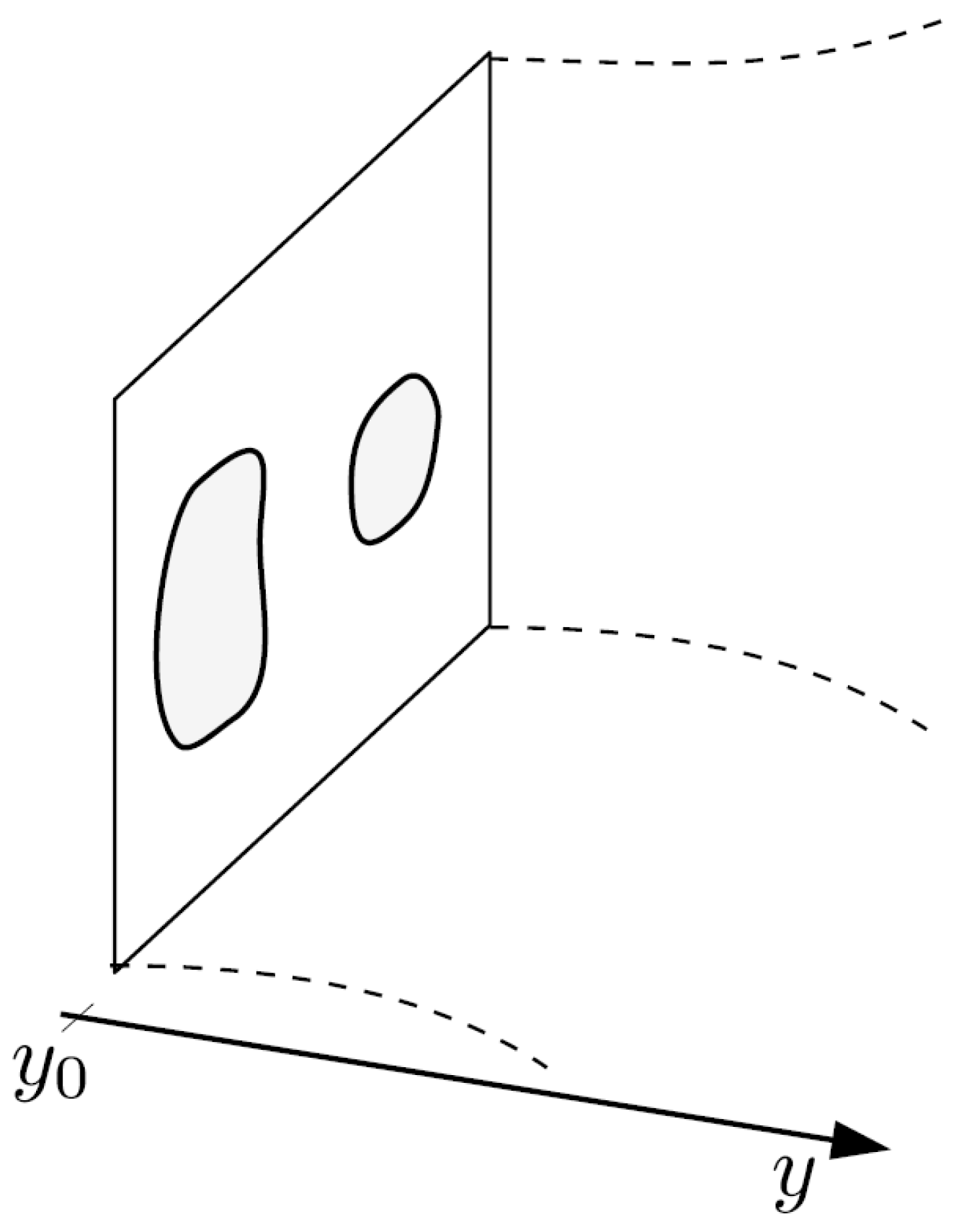
Using Equation (29), one sees that this corresponds to a boundary-localized mass term for $\Phi$ on the AdS side. Therefore, the double-trace deformation on the CFT side is encoded as a deformation of the boundary condition of $\Phi$ on the AdS side. The double-trace defect of the CFT is realized as a boundary mass term with a support that is localized along the boundary volume. In brief, the defect is on the boundary (Figure 2).

The domain for which the ${\Delta }_{-}$ correspondence applies is precisely the range given in Equation (14). Thus, our model of defect CFT can always be realized holographically from the AdS viewpoint: the double-trace deformation defined via AdS is automatically relevant.

At the level of the vacuum energies, we have the identification

$$E_{\mathrm{CFT}}\left[J\right]=E_{\mathrm{AdS}}\left[J\right]$$

(31)

with

$$E_{\mathrm{AdS}}\left[J\right]=iTlog{Z}_{\mathrm{AdS}}\left[J\right],Z_{\mathrm{AdS}}\left[J\right]=\int \mathcal{D}{\Phi }_0{e}^{i{\int }_{\partial }{d}^{d}x\frac{\xi }{2}J\left(\mathit{x}\right){\Phi }_0^2}{\int }_{{\Phi }_0}\mathcal{D}\Phi e^{i{S}_{\mathrm{AdS}}[\Phi ]}.$$

(32)

When the correspondence (31) holds, applying the functional formalism of Section 2.2 to $E_{\mathrm{CFT}}$ means on the AdS side that we deform the support of the boundary-localized mass term. In other words, the boundary condition for the bulk fields gets deformed. The phenomenon of the 2-point correlator being repelled from the defect in the IR is understood on the AdS side as the bulk field being repelled from the boundary due to the mass term. For $\xi \to \infty$, the AdS propagator vanishes on the boundary of the defect localized on the AdS boundary.

We do not use further the AdS picture in the following.

4. A CFT between Two Membranes

We explore further the properties of the 2-point CFT correlators in the presence of two double-trace membranes. The full defect is given by

$$J\left(\mathit{x}\right)=J_a\left(\mathit{x}\right)+J_b\left(\mathit{x}\right)=\frac{{\xi }_a}{2}\delta (z-z_a)+\frac{{\xi }_b}{2}\delta (z-z_b).$$

(33)

We define $|z_b-z_a|=L$. A convenient way to obtain the 2-point function is by dressing it successively with the two membranes $J_a$ and $J_b$. We obtain

$$G_a(p;z_1,z_2)=G(p;z_1,z_2)+G(p;z_1,z_a)\frac{{\xi }_a}{1-{\xi }_{a}G(p;z_a,z_a)}{G}_0(p;z_a,z_2),$$

(34)

$$\begin{array}{ccc}\hfill & & G_{a,b}(p;z_1,z_2)=G_a(p;z_1,z_2)+G_a(p;z_1,z_b)\frac{{\xi }_b}{1-{\xi }_b{G}_a(p;z_b,z_b)}{G}_a(p;z_b,z_2)\hfill \\ & & =G_{12}+\frac{{\xi }_b{G}_{1b}\left({\xi }_a{G}_{ab}{G}_{a2}+(1-{\xi }_a{G}_0)G_{b2}\right)+{\xi }_a{G}_{1a}({\xi }_b{G}_{ab}{G}_{b2}+(1-{\xi }_b{G}_0)G_{a2})}{({\xi }_a{G}_0-1)({\xi }_b{G}_0-1)-{\xi }_a{\xi }_b{G}_{ab}^2}.\hfill \end{array}$$

(35)

In the second line of Equation (35), we introduce the notation $G(p;z_i,z_j)\equiv G_{ij}$.

4.1. Dirichlet Limit

To understand the behavior of this 2-point function, we take the ${\xi }_{a,b}\to \infty$. At finite ${\xi }_{a,b}$, this corresponds to the asymptotic limit associated to the infrared regime. In this limit, the CFT gets literally confined inside the $[0,L]$ interval. The 2-point correlator becomes

$$G_{\mathrm{D}}(p;z_1,z_2)=G_{12}+\frac{G_{1b}{G}_{ab}{G}_{a2}-G_{1b}{G}_0{G}_{b2}+G_{1a}{G}_{ab}{G}_{b2}-G_{1a}{G}_0{G}_{a2}}{G_0^2-G_{ab}^2}.$$

(36)

4.2. Poles

We stay in the Dirichlet limit for simplicity. Due to the denominator in Equation (36), it turns out that $G_D$ features a series of poles in the complex plane of p determined by the condition

$$G(p;z_a,z_b)=\pm G_0\left(p\right).$$

(37)

Explicitly, the poles in p are determined by solving

$$\frac{1}{\Gamma \left(\alpha \right)}{\left(\sqrt{-p^2}L\right)}^{\alpha }{K}_{\alpha }\left(\sqrt{-p^2}L\right)=\pm 1,\alpha =\frac{d-1}{2}-\Delta ,$$

(38)

with $-\frac{1}{2}<\alpha <\frac{1}{2}$. We denote the complex values of p solving Equation (38) by $m_n^{\pm }$. There is no massless pole ($p=0$) nor light pole ($p\ll 1/L$) thanks to the asymptotic behavior at relatively small p is $G_{ab}\to G_0$ (see Equation (22)), in which case Equation (37) is either trivial or impossible to satisfy.

4.3. Residues

The residues associated to the $p=m_n^{\pm }$ poles take quite a simple factorized form, $(G_{a1}\mp G_{b1})(G_{a2}\mp G_{b2})$,

$$G(p;z_1,z_2)\stackrel{p\sim m_n^{\pm }}{\approx }-\frac{1}{2}\frac{f_n^{\pm }\left(z_1\right)f_n^{\pm }\left(z_2\right)}{G_{ab}\mp G_0},f_n\left(z\right)\equiv G(m_n^{\pm },z,z_a)\mp G(m_n^{\pm },z,z_b).$$

(39)

This factorized form is reminiscent of weakly coupled QFT on an interval, which develops a sequence of discrete modes. In the weakly coupled case, the poles lie on the real line up to the corrections due to the interactions. Equation (39) then corresponds to the Kállen–Lehmann representation of the propagator confined in the $[0,L]$ interval. Here, we see that the factorized structure remains true even if the poles lie anywhere in the complex plane.

4.4. Free Limit

In the case of the free field in $d=4$, we have $\Delta =1$. The 2-point correlator becomes

$$i{G}^{\mathrm{free}}(p;z_1,z_2)=-i4{\pi }^{2}a\frac{e^{-\sqrt{-p^2}|z_1-z_2|}}{2\sqrt{-p^2}},$$

(40)

where, for a canonically normalized field, $a=1/\left(4{\pi }^2\right)$. In this case, the poles determined by Equation (38) are real, with $m_n^{\mathrm{free}}=n\pi /L$, $n\in {\mathbb{N}}^{★}$. The propagator dressed by the two membranes takes the form

$$i{G}^{\mathrm{free}}(p;z_1,z_2)=i\frac{sinh\left(\sqrt{-p^2}(z_a-z_{<})\right)sinh\left(\sqrt{-p^2}(z_{>}-z_b)\right)}{\sqrt{-p^2}sinh\left(\sqrt{-p^2}(z_b-z_a)\right)},$$

(41)

where we assume $z_a<z_b$ and define $z_{<(>)}=min(max)(z,z^{\prime })$. This matches the result obtained by solving the free field equation of motion on the interval with Dirichlet boundary conditions on the membranes (see, for example, the Appendix of Ref. [63]).

4.5. Resonances

Slightly away from the free field case, for $\Delta -(d-2)/2\ll 1$, it turns out that the set of poles of the CFT behaves as a tower of narrow resonances at values $p=m_n\equiv m_n^{\mathrm{free}}-i{\Gamma }_n/2$ with ${\Gamma }_n\ll m_n^{\mathrm{free}}$. Expanding the relation (38), we find that the resonances feature a common decay rate ${\Gamma }_n$:

$${\Gamma }_n\approx \left(\Delta -\frac{d-2}{2}\right)\pi /L.$$

(42)

Details of the computation are given in Appendix A.

One obtains, thus, a notion of unstable particle states directly from a CFT. Since the CFT has internal degrees of freedom, one may think of these resonances as collective excitations. The fact that the resonances decay reflects the fact that, for $\Delta >(d-2)/2$, the theory is interacting. However, the decay width is independent of the underlying physics of the CFT; it is controlled by the dimension of the double-trace operator that causes the CFT confinement on the interval.

5. CFT Casimir Forces between Defects and Boundaries

We compute the quantum forces induced by the CFT between localized double-trace operators with pointlike and planar supports. The planar geometry includes the case of a flat boundary (for example, $z>0$) of a membrane and also the case of a plate of any width. We consider two disjoint defects, described by

$$S=S_{\mathrm{CFT}}-\frac{1}{2}\int d^{d}x{\mathcal{O}}^2\left(x\right)J\left(\mathit{x}\right),J\left(\mathit{x}\right)={\xi }_a{J}_a\left(\mathit{x}\right)+{\xi }_b{J}_b\left(\mathit{x}\right).$$

(43)

The ${\xi }_{a,b}$ parameters have mass dimension: $\left[{\xi }_{a,b}\right]=d-\left[J_{a,b}\right]-2\Delta$.

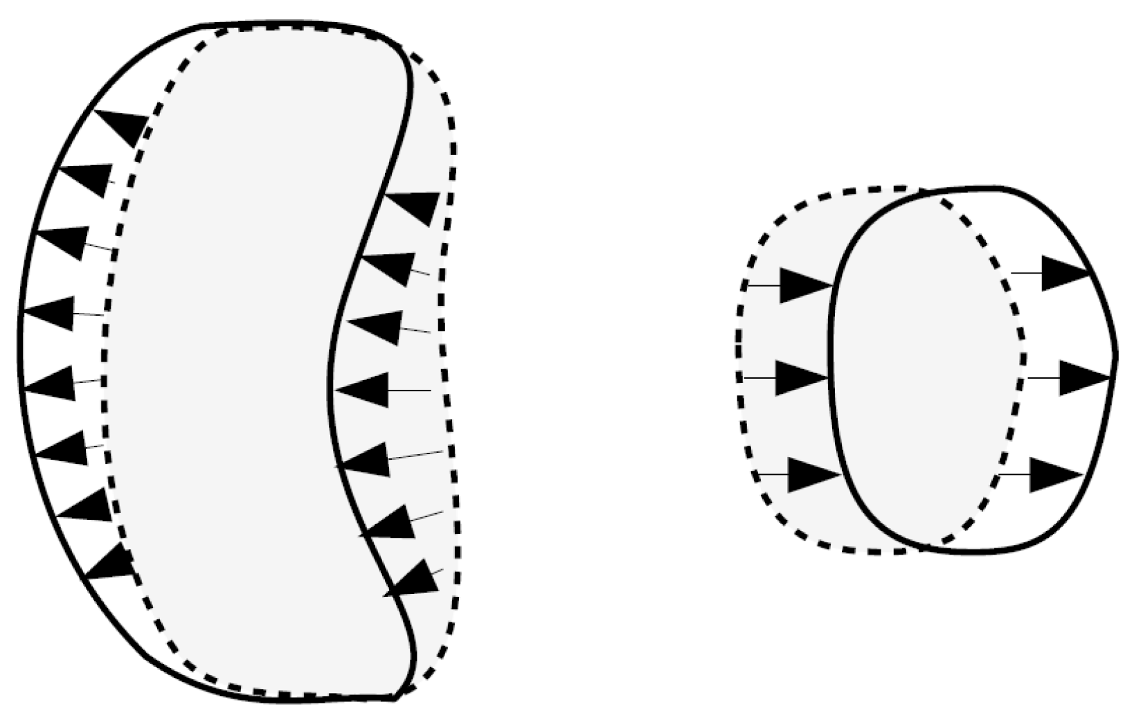
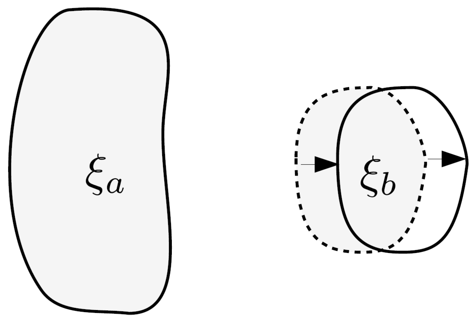
We consider a rigid deformation of J such that $J_b$ gets shifted along a constant $\mathbf{L}$ while $J_a$ remains identical,

$$J_{a,\lambda +d\lambda }\left(\mathit{x}\right)=J_{a,\lambda }\left(\mathit{x}\right),J_{b,\lambda +d\lambda }\left(\mathit{x}\right)=J_{b,\lambda }(\mathit{x}-\mathbf{L}d\lambda ),$$

(44)

exemplified as shown in Figure 3.

The quantum work is then expressed as

$$W=-\frac{{\xi }_b}{2}\int d^{d-1}\mathit{x}{\langle \mathcal{O}\left(x\right)\mathcal{O}\left(x\right)\rangle }_J{\partial }_{\lambda }{J}_{b,\lambda }\left(\mathit{x}\right).$$

(45)

Equation (45) is the formula we apply throughout this Section.

The CFT propagator in the presence of J can always be written in the form of a Born series as described in Equation (19). Evaluating the expression in a closed form for, for example, a plate is more challenging. Here, we limit ourselves to computing analytical results for the force between $J_a$ and $J_b$ in two limiting cases: the asymptotic Casimir–Polder and Casimir regimes.

5.1. CFT Casimir–Polder Forces

In the UV regime, i.e., in the limit of short separation, the effect of the J insertion in the Born series tends to be quite small. In this limit, the first terms of the series dominate. It turns out that the leading contribution to the quantum work is [34]

$$\begin{array}{ccc}\hfill W& =& -i\frac{{\xi }_a{\xi }_b}{2}\int d^{d-1}\mathit{x}{d}^d{x}^{\prime }\langle \mathcal{O}\left(x^{\prime }\right)\mathcal{O}\left(x\right)\rangle J_a\left(\mathit{x}\right)\langle \mathcal{O}\left(x\right)\mathcal{O}\left(x^{\prime }\right)\rangle \mathbf{L}·\partial J_b\left({\mathit{x}}^{\prime }\right)+O\left({\xi }^3\right).\hfill \end{array}$$

(46)

Upon integration by part, we recognize the structure of a potential $W=-\mathbf{L}·\partial V_{ab}$ with

$$V_{ab}=-i\frac{{\xi }_a{\xi }_b}{2}\int d^{d-1}\mathit{x}{d}^{d-1}{\mathit{x}}^{\prime }{J}_a\left(\mathit{x}\right)J_b\left({\mathit{x}}^{\prime }\right)\int dt{\langle \mathcal{O}(0,\mathit{x})\mathcal{O}(t,{\mathit{x}}^{\prime })\rangle }^2.$$

(47)

The $V_{ab}$ potential has a Casimir–Polder-like structure; it is a loop made of two CFT correlators that connects the two defects. Hence, we refer to this limit as the Casimir–Polder limit.

5.1.1. Point–Point Geometry

We first consider two defects that are pointlike,

$$J_a\left(\mathit{x}\right)={\delta }^{d-1}\left(\mathit{x}\right),J_b\left(\mathit{x}\right)={\delta }^{d-1}(\mathit{x}-\mathit{r}).$$

(48)

The potential becomes

$$V\left(r\right)=-i\frac{{\xi }_a{\xi }_b}{2}\int dt{\langle \mathcal{O}\left(0\right)\mathcal{O}(t,r)\rangle }^2,$$

(49)

with $r=\left|\mathit{r}\right|$.

We compute Equation (49) by going to the full momentum space. The momentum space correlator is Equation (3). In momentum space, the potential is given by

$$V\left(p\right)=i\frac{{\xi }_a{\xi }_b}{2}\frac{{\pi }^d{\Gamma }^2(d/2-\Delta )}{{\Gamma }^2(\Delta )}\int \frac{d^{d}k}{{\left(2\pi \right)}^d}{\left(\frac{4}{-k^2}\right)}^{d/2-\Delta }{\left(\frac{4}{-{(k+p)}^2}\right)}^{d/2-\Delta },$$

(50)

where $p_0=0$. We rotate the integral to Euclidean space with Euclidean momentum $q^M$ satisfying $q^2=-k^2$, and go to spherical coordinates,

$$V\left(p\right)=-\frac{{\xi }_a{\xi }_b}{2}\frac{{\pi }^d{\Gamma }^2(d/2-\Delta )}{{\Gamma }^2(\Delta )}\int \frac{d^{d}q}{{\left(2\pi \right)}^d}{\left(\frac{4}{q^2}\right)}^{d/2-\Delta }{\left(\frac{4}{{(q+p)}^2}\right)}^{d/2-\Delta }.$$

(51)

We need to evaluate

$$\begin{array}{c}\hfill \int \frac{d^{d}q}{{\left(2\pi \right)}^d}{\left({\left(p+q\right)}^2\right)}^a{\left(q^2\right)}^b,\end{array}$$

(52)

for some $a,b$. We apply the identity

$$\begin{array}{c}\hfill {\left({\left(p+q\right)}^2\right)}^a{\left(q^2\right)}^b={\int }_0^{1}dx\frac{{(x{\left(p+q\right)}^2+(1-x)q^2)}^{a+b}}{x^{a+1}{(1-x)}^{b+1}}\frac{\Gamma (-a-b)}{\Gamma (-a)\Gamma (-b)}.\end{array}$$

(53)

The integral on the right-hand side converges for $\mathrm{Re}\left(a\right),\mathrm{Re}\left(b\right)<0$. However, provided the final result of the calculation is analytic in $a,b$, the result can be extended by analytical continuation such that restrictions on $a,b$ are ultimately lifted. Shifting the loop momentum $l\equiv q+px$, one obtains for Equation (52):

$$\begin{array}{c}\hfill {\int }_0^{1}dx\int \frac{d^{d}l}{{\left(2\pi \right)}^d}\frac{{(l^2+x(1-x)p^2)}^{a+b}}{x^{a+1}{(1-x)}^{b+1}}\frac{\Gamma (-a-b)}{\Gamma (-a)\Gamma (-b)}.\end{array}$$

(54)

We evaluate the loop integral with

$$\begin{array}{c}\hfill \int \frac{d^{d}l}{{\left(2\pi \right)}^d}{\left(l^2+\Delta \right)}^c=\frac{\Gamma \left(-c-\frac{d}{2}\right)}{\Gamma (-c)}\frac{{\Delta }^{c+d/2}}{{\left(4\pi \right)}^{d/2}}.\end{array}$$

(55)

Again, the loop integrals are performed in the domain of $(c,d)$, where the integral on the left-hand side converges. The functions on the right-hand side are analytic in c anywhere away from the integral values of c; hence, the final result will be ultimately analytically continued in c. For certain values of $\Delta$ at even d, a physical divergence appears, which requires renormalization. However, such divergences are irrelevant for our study as soon as it is ultimately only the branch cut of $V\left(p\right)$ that contributes to the spatial potential; see [64]. Hence, no divergence appears in the position space propagators when $\Delta$ is set to integer values.

Putting Equations (53) and (55) together yields for Equation (52):

$$\begin{array}{c}\hfill \frac{1}{{\left(4\pi \right)}^{\frac{d}{2}}}{\left(p^2\right)}^{a+b+\frac{d}{2}}\frac{\Gamma \left(-a-b-\frac{d}{2}\right)}{\Gamma (-a)\Gamma (-b)}{\int }_0^{1}dx{x}^{b+\frac{d}{2}-1}{(1-x)}^{a+\frac{d}{2}-1}.\end{array}$$

(56)

We identify the remaining integral as being the integral representation of the Beta function. Evaluating the integral, one obtains for Equation (52):

$$\begin{array}{c}\hfill \frac{1}{{\left(4\pi \right)}^{d/2}}{\left(p^2\right)}^{a+b+d/2}\frac{\Gamma (-a-b-d/2)}{\Gamma (-a)\Gamma (-b)}\frac{\Gamma (a+d/2)\Gamma (b+d/2)}{\Gamma (a+b+d)}.\end{array}$$

(57)

The potential in momentum space is thus

$$V\left(p\right)=-\frac{{\xi }_a{\xi }_b}{2}\frac{{\pi }^d{\Gamma }^2(d/2-\Delta )}{{\Gamma }^2(\Delta )}{4}^{d-2\Delta }\frac{1}{{\left(4\pi \right)}^{d/2}}{\left(p^2\right)}^{2\Delta -d/2}\frac{\Gamma (-2\Delta +d/2)}{\Gamma (\frac{d}{2}-\Delta )\Gamma (\frac{d}{2}-\Delta )}\frac{{\Gamma }^2(\Delta )}{\Gamma (2\Delta )}.$$

(58)

Simplifying,

$$V\left(p\right)=-\frac{{\xi }_a{\xi }_b}{2}{\left(\frac{p^2}{4}\right)}^{2\Delta -d/2}\frac{{\pi }^{d/2}\Gamma (-2\Delta +d/2)}{\Gamma (2\Delta )}.$$

(59)

We can recognize that Equation (59) is proportional to the momentum space 2-point correlator of the double-trace operator ${\mathcal{O}}^2$ with $p_0=0$. That is, due to the properties of the CFT, the loop of $\mathcal{O}$ can be understood as a tree exchange of ${\mathcal{O}}^2$. (Particle physics models involving such processes have been considered in Refs. [65,66,67].) The overall coefficient is nontrivial; however, our loop calculation is required to determine it. This phenomenon occurs only in the Casimir–Polder regime.

One may notice that the numerator diverges if $\Delta \to d/4$, which is allowed when $d\le 4$ since $\Delta \ge (d-2)2$. However, the expression for the potential in position space computed below is automatically finite even in the case $\Delta \to d/4$, This is because this is a quantity computed at separated points. Keeping a general, non-integer, dimension $\Delta$ throughout the calculation plays the same role as dimensional regularization weakly coupled QFT. Finally, we can go back to position space with a $(d-1)$ Fourier transform, $V\left(r\right)=\int \frac{d^{d-1}p}{{\left(2\pi \right)}^{d-1}}{e}^{ipr}V\left(p\right)$. We obtain the final result for the CFT Casimir–Polder potential between two pointlike double-trace deformations,

$$V\left(r\right)=-\sqrt{\pi }\frac{{\xi }_a{\xi }_b}{2}\frac{\Gamma (2\Delta -\frac{1}{2})}{\Gamma (2\Delta )}\frac{1}{r^{4\Delta -1}}.$$

(60)

As a cross check, taking $\Delta =1$ and using the $a=\frac{1}{4\pi }$ normalization for each correlator, we recover exactly the Casimir–Polder potential from the exchange of 4D free massless scalars, $V\left(r\right)=-{\xi }^2/\left(64{\pi }^3{r}^3\right)$. Notice that $\left[{\xi }_{a,b}\right]=1-2\Delta$; thus, $\left[V\right]=1$.

5.1.2. Point–Plate

We calculate the Casimir–Polder potential between a point particle and an infinite plate located at $z<0$. In terms of the support functions, this is described by

$$J_a\left(\mathit{x}\right)=\Theta (-z),J_b\left(\mathit{x}\right)={\delta }^{d-2}\left({\mathit{x}}_{\Vert }\right)\delta (z-\ell ),$$

(61)

where $\Theta (·)$ is the Heaviside function.

We assume that the deformation moves $J_b$ along the z direction, i.e., $\mathbf{L}=(\mathbf{0},1)$. The $x_{\Vert }$ are the coordinates parallel to the plate.

The CFT force between the point and the membrane can be straightforwardly obtained by integrating the point–point Casimir–Polder potential over $J_a$. This simplified approach is valid only in the Casimir–Polder limit. The ${\xi }_{a,b}$ are defined such that the parametrization (43) holds, now with the defect (61). ${\xi }_a$ is related to the pointlike source coupling by ${\xi }_a=n{\xi }_a^{\mathrm{point}}$, where n is the number density of $J_a$.

The Casimir–Polder force is given by the potential

$$V(\ell )=n{\int }_{-\infty }^{0}dz\int d^2{x}_{\Vert }\int \frac{d^{3}p}{{\left(2\pi \right)}^3}{e}^{i{p}_z(\ell -z)}{e}^{i{p}_{\Vert }.x_{\Vert }}V\left(p\right).$$

(62)

The $p_{\Vert }$ is the momentum component along the plate. The integral reduces to

$$V(\ell )=-\frac{{\pi }^{d/2}{\xi }_a{\xi }_b}{2}\frac{\Gamma (-2\Delta +d/2)}{\Gamma (2\Delta )}{\int }_{-\infty }^{0}dz\int \frac{d{p}_z}{2\pi }{e}^{i{p}_z(\ell -z)}{\left(\frac{p^2}{4}\right)}^{2\Delta -d/2}.$$

(63)

The momentum integral can be performed and gives

$$\int \frac{d{p}_z}{2\pi }{e}^{i{p}_z(\ell -z)}{\left(\frac{p^2}{4}\right)}^{2\Delta -d/2}=\frac{\Gamma (2\Delta +\frac{1-d}{2})}{\sqrt{\pi }\Gamma (\frac{d}{2}-2\Delta )}\frac{1}{{(\ell -z)}^{4\Delta +1-d}}.$$

(64)

The integral over z converges, provided $\Delta >d/4$. When computing the force further below, the divergence matters only when for a free field in $d=3$. In the convergent case, we have

$$V(\ell )=-\frac{{\pi }^{(d-1)/2}}{2(4\Delta -d)}\frac{\Gamma (2\Delta +\frac{1-d}{2})}{\Gamma (2\Delta )}\frac{{\xi }_a{\xi }_b}{{\ell }^{4\Delta -d}},$$

(65)

where $d>4$. The force is then given by $F=-\partial V/\partial \ell$, which gives

$$F(\ell )=-\frac{{\pi }^{(d-1)/2}\Gamma (2\Delta +\frac{1-d}{2})}{2\Gamma (2\Delta )}\frac{{\xi }_a{\xi }_b}{{\ell }^{4\Delta -d+1}}.$$

(66)

For a free field in $d=4$, one obtains

$$F(\ell )=-\frac{{\pi }^2}{2}\frac{{\xi }_a{\xi }_b}{\ell }.$$

(67)

This correctly reproduces the $\propto \frac{1}{\ell }$ scalar Casimir–Polder force derived in Ref. [34], $-\frac{{\xi }_a{\xi }_b}{32{\pi }^2\ell }$, once one takes into account the canonical normalization of the free fields, which introduces the factor $a^2={\left(\frac{1}{4{\pi }^2}\right)}^2$. (A factor of $\frac{1}{2}$ is missing in Equation (6.29) of Ref. [34]).

The case of the free field in $d=3$ necessitates the assumption that the plane has finite width L. We obtain

$$F(\ell )=-\frac{\pi \Gamma (2\Delta -1)}{2\Gamma (2\Delta )}{\xi }_a{\xi }_{b}log\left(1+\frac{L}{\ell }\right).$$

(68)

5.1.3. Plate–Plate CFT Casimir–Polder

We similarly compute the Casimir–Polder pressure between two infinite plates. This is described by

$$J_a\left(\mathit{x}\right)=\Theta (-z),J_b\left(\mathit{x}\right)=\Theta (z-\ell ).$$

(69)

We assume that the deformation moves $J_b$ along the z direction, i.e., $\mathbf{L}=(\mathbf{0},1)$. (In general, one should require that the plates end far away, i.e., are not formally infinite, in order for the deformation flow to be divergence-free [34]; while this is necessary in general, this detail does not affect the present Casimir–Polder calculation.)

The ${\xi }_{a,b}$ are defined such that the parametrization Equation (43) holds, now in the presence of the defect (61). ${\xi }_{a,b}$ is related to the pointlike source coupling by ${\xi }_{a,b}=n_{a,b}{\xi }_{a,b}^{\mathrm{point}}$ with $n_{a,b}$, the number density of $J_{a,b}$. Similarly to the point–plate case, we integrate the point–point potential over the two defects, with, for example,

$$F_{\mathrm{plate}-\mathrm{plate}}(\ell )=-n_b{S}_{d-2}{\int }_{\ell }^{\infty }dz{F}_{\mathrm{point}-\mathrm{plate}}\left(z\right),$$

(70)

where $S_{d-2}=\int d^{d-2}{\mathit{x}}_{\Vert }$ is the volume integral in Equation (70) in the directions parallel to the plate. As long as $\Delta >d/4$, the integral is IR convergent and gives

$$\frac{F(\ell )}{S_{d-2}}=-\frac{{\pi }^{(d-1)/2}}{2(4\Delta -d)}\frac{\Gamma (2\Delta +\frac{1-d}{2})}{\Gamma (2\Delta )}\frac{{\xi }_a{\xi }_b}{{\ell }^{4\Delta -d}}.$$

(71)

The case of a free field in $d=4$ is logarithmically divergent. This is a physical divergence that signals that we should consider finite plates instead of approximating them as infinite. It is sufficient to assume that one of the plates, here, the second plate integrated in Equation (70), has finite width L. We find

$$\frac{F(\ell )}{S_1}=-\frac{{\pi }^2}{2}{\xi }_a{\xi }_{b}ln\left(1+\frac{L}{\ell }\right).$$

(72)

The IR divergent behavior also appears in the result of Ref. [34], in the case where the free field is massless. There is no IR divergence if the free field is massive.

5.2. CFT Casimir Forces

We compute forces beyond the Casimir–Polder approximation. Our focus is on membranes. Computing analytical results for plates of finite widths is more challenging. However, in the IR regime for which the plate width is smaller than other distance scales of the problem, we expect the results to reproduce the one obtained with membranes.

Since the chosen defects feature membranes, we restrict $\Delta$ to the interval (24). The case $\Delta \ge (d-1)2$ deserves a separate analysis.

5.2.1. Point–Membrane CFT Casimir

We first compute the force between a membrane at $z=0$ and a point at distance $z=\ell$. The two defects are parametrized as

$$J_a\left(\mathit{x}\right)=\delta \left(z\right),J_b\left(\mathit{x}\right)={\delta }^{d-2}\left({\mathit{x}}_{\Vert }\right)\delta (z-\ell ).$$

(73)

The membrane is infinitely thin in contrast with the point–plate case of the previous section, where the plate had a large width. We choose that the deformation moves the pointlike defect along z, while the membrane stays in place, i.e., it is given by Equation (44), where $\mathbf{L}$ is oriented along z. The deformation of the defect is then given by

$${\partial }_{\lambda }J=-{\xi }_{b}L{\delta }^{d-2}\left({\mathit{x}}_{\Vert }\right){\partial }_z\delta (z-\ell ).$$

(74)

The quantum force is given by

$$\begin{array}{ccc}\hfill F(\ell )& =& -\frac{1}{2}\int d^{d-1}\mathit{x}{\langle \mathcal{O}\left(x\right)\mathcal{O}\left(x\right)\rangle }_J{\partial }_{\lambda }{J}_{b,\lambda }\left(\mathit{x}\right)\hfill \end{array}$$

(75)

$$\begin{array}{ccc}& =& -\frac{{\xi }_b}{2}{\partial }_z{\langle \mathcal{O}(x^{\alpha },z)\mathcal{O}(x^{\alpha },z)\rangle }_J{|}_{z\to \ell }.\hfill \end{array}$$

(76)

Here, ${\langle \mathcal{O}(x^{\alpha },z)\mathcal{O}(x^{\alpha },z)\rangle }_J$ is the CFT 2-point function dressed by the membrane at $z=0$. This correlator is computed in Equation (26). Going to the position–momentum space, one has

$$G_J(p;z,z)=G_0\left(p\right)+G^2(p;0,z)\frac{{\xi }_a}{1-{\xi }_a{G}_0\left(p\right)},$$

(77)

where $G_0\left(p\right)$ is defined in Equation (27).

The quantum force is then expressed as

$$\begin{array}{ccc}\hfill F(\ell )& =& -\frac{i{\xi }_b}{2}\int \frac{d^{d-1}p}{{\left(2\pi \right)}^{d-1}}{\partial }_z{G}_J(p;z,z){|}_{z\to \ell }\hfill \end{array}$$

(78)

$$\begin{array}{ccc}& =& -\frac{i}{2}\int \frac{d^{d-1}p}{{\left(2\pi \right)}^{d-1}}\frac{{\xi }_a{\xi }_b}{1-{\xi }_a{G}_0\left(p\right)}{\partial }_z{\left(G^2(p;0,z)\right)}_{z\to \ell },\hfill \end{array}$$

(79)

where $G_0\left(p\right)$ does not contribute since it is constant in z.

The derivative piece takes a straightforward form:

$${\partial }_z{\left(G^2(p;0,z)\right)}_{z\to \ell }=-\frac{16{\pi }^{d-1}\ell }{{\Gamma }^2(\Delta )}{\left(\frac{4{\ell }^2}{-p^2}\right)}^{\frac{d-2-2\Delta }{2}}{K}_{\frac{1-d}{2}+\Delta }\left(\sqrt{-p^2}\ell \right)K_{\frac{3-d}{2}+\Delta }\left(\sqrt{-p^2}\ell \right).$$

(80)

One may notice it is proportional to the product of two correlators with dimension $\Delta$ and $\Delta +1$.

We can identify the potential directly from the line (79), where the ${\partial }_z$ derivative is equivalent to ${\partial }_{\ell }$. We rotate to Euclidean momentum $q^M$ and use spherical coordinates. We find the general result:

$$V(\ell )=-\frac{{\pi }^{\frac{d-1}{2}}}{2^{d-3}\Gamma \left(\frac{d-1}{2}\right){\Gamma }^2(\Delta )}\int dq{q}^{d-2}\frac{{\xi }_a{\xi }_b}{1-{\xi }_b{G}_0\left(q\right)}{\left(\frac{2\ell }{q}\right)}^{d-1-2\Delta }{K}_{\frac{1-d}{2}+\Delta }^2\left(q\ell \right),$$

(81)

$$F(\ell )=-\frac{{\pi }^{\frac{d-1}{2}}\ell }{2^{d-5}\Gamma \left(\frac{d-1}{2}\right){\Gamma }^2(\Delta )}\int dq{q}^{d-2}\frac{{\xi }_a{\xi }_b}{1-{\xi }_b{G}_0\left(q\right)}{\left(\frac{2\ell }{q}\right)}^{d-2-2\Delta }{K}_{\frac{1-d}{2}+\Delta }\left(q\ell \right)K_{\frac{3-d}{2}+\Delta }\left(q\ell \right).$$

(82)

One can evaluate the loop integral in both the Casimir–Polder regime ${\xi }_a{G}_0\left(p\right)\ll 1$ and the Casimir regime ${\xi }_a{G}_0\left(p\right)\gg 1$. We write the two Bessel functions using the representation (6), and perform the loop momentum integral and then the t and $t^{\prime }$ integrals. The intermediate steps involve hypergeometric functions, but the final results are remarkably simple.

In the Casimir–Polder regime, we obtain the potential

$$V(\ell )=-\frac{{\pi }^{(d-1)/2}\Gamma (2\Delta +\frac{1-d}{2})}{2\Gamma (2\Delta )}\frac{{\xi }_a{\xi }_b}{{\ell }^{4\Delta -d+1}}.$$

(83)

It is attractive for any $\Delta$ satisfying the unitarity bound. For $d=3$ and 4 the Casimir–Polder force is

$$F_{d=3}(\ell )=-\frac{\pi {\xi }_a{\xi }_b}{{\ell }^{4\Delta -1}}\mathrm{and}$$

(84)

$$F_{d=4}(\ell )=\frac{{\pi }^{3/2}\Gamma (2\Delta -\frac{1}{2})}{\Gamma (2\Delta )}\frac{{\xi }_a{\xi }_b}{{\ell }^{4\Delta -2}},$$

(85)

respectively.

For the free field in $d=4$, including two factors of $a=\frac{1}{4{\pi }^2}$ to recover canonical normalization, we find $F(\ell )=-\frac{{\xi }_a{\xi }_b}{32{\pi }^2{\ell }^2}$. Notice that this Casimir–Polder limit corresponds to a loop between a point and an infinitely thin membrane; it differs from the point–plate geometry of Section 5.1.2, where the width of the plate is quite large.

In the Casimir regime, one obtains

$$V(\ell )=-\frac{\sqrt{\pi }d\Gamma (d-1-\Delta )}{2^d\Gamma (1+\frac{d}{2})\Gamma \left(\frac{d-1-2\Delta }{2}\right)}\frac{{\xi }_b}{{\ell }^{2\Delta }}.$$

(86)

The potential depends only on ${\xi }_b$ and is attractive for $\Delta$ in the interval of interest, $\frac{d-2}{2}\le \Delta <\frac{d-1}{2}$. For $d=3$ and 4, one obtains the forces

$$F_{d=3}(\ell )=\Delta (\Delta -1)\frac{{\xi }_b}{{\ell }^{2\Delta +1}}\mathrm{and}$$

(87)

$$F_{d=4}(\ell )=-\frac{\sqrt{\pi }\Delta \Gamma (3-\Delta )}{4\Gamma (\frac{3}{2}-\Delta )}\frac{{\xi }_b}{{\ell }^{2\Delta +1}},$$

(88)

respectively.

For the free field in $d=4$, including one factor of $a=\frac{1}{4{\pi }^2}$ to recover canonical normalization, one finds $F(\ell )=-{\xi }_b/\left(16{\pi }^2{\ell }^3\right)$. This reproduces exactly the Casimir force obtained from the plate–point configuration taken in the Dirichlet limit computed in Ref. [34]. This illustrates that, in the Casimir regime, only the boundary of the defect matters. The $V(\ell )\propto {\ell }^{-2\Delta }$ dependence in the Casimir regime is reminiscent of the feature that the ${\mathcal{O}}^2$ operator in a boundary CFT admits a vev with profile $\langle {\mathcal{O}}^2\rangle \propto z^{-2\Delta }$.

5.2.2. Membrane–Membrane CFT Casimir

We turn to the force between two membranes at $z=0$ and $z=\ell$. The two defects are parametrized as

$$J_a\left(\mathit{x}\right)=\delta \left(z\right),J_b\left(\mathit{x}\right)=\delta (z-\ell ).$$

(89)

The deformation of the defect is given by

$${\partial }_{\lambda }J=-{\xi }_{b}L{\partial }_z\delta (z-\ell ).$$

(90)

Following the same steps as in Section 5.1.1, we arrive at the quantum pressure

$$\frac{F(\ell )}{S_{d-2}}=-\frac{i{\xi }_b}{2}\int \frac{d^{d-1}p}{{\left(2\pi \right)}^{d-1}}{\partial }_z{G}_J(p;z,z){|}_{z\to \ell },$$

(91)

with $S_{d-2}=\int d^{d-2}{\mathit{x}}_{\Vert }$. The 2-point correlator in the presence of two membranes is computed in Equation (35).

Unlike in the other cases previously treated (see Equation (81)), it is not possible to identify a potential directly from Equation (91). This is due to the feature that the ${\partial }_z$ derivative cannot be traded for a derivative in ℓ as soon as the dressed 2-point correlator depends nontrivially on ℓ; see Equation (35). Rather, we first compute the force, which is the fundamental quantity, then one may optionally infer a potential from it.

Our focus is on the Casimir limit, which amounts to taking quite large ${\xi }_{a,b}$. Notice that one cannot use in Equation (91) the Dirichlet limit (36), for which ${\xi }_{a,b}=\infty$. This would lead to an indefinite $0\times \infty$ form in Equation (91). Instead, one should compute the expansion of $G_J$ for relatively large but finite ${\xi }_{a,b}$. The self-consistency of the quantum work formalism ensures that this expansion and the ${\xi }_b$ factor in Equation (91) will conspire to give a finite result for the pressure.

One finds

$${\partial }_z{G}_J(p;z,z){|}_{z\to \ell }=\frac{1}{{\xi }_b}\frac{{\partial }_z{\left(G^2(0,z)\right)}_{z\to \ell }}{G_0^2\left(p\right)-G^2(p;0,\ell )}+O\left(\frac{1}{{\xi }_a},\frac{1}{{\xi }_b^2}\right).$$

(92)

To obtain this result, we use that ${\partial }_{z}G(p;z,z^{\prime }){|}_{z^{\prime }\to z}=0$ by symmetry. This sets to zero the would-be leading term ${\xi }_{a,b}^0$. As a result, the $1/{\xi }_b$ term is the leading one.

The quantum pressure between the membranes is then

$$\frac{F(\ell )}{S_{d-2}}=\frac{{\pi }^{\frac{d-1}{2}}}{2^{d-1}\Gamma \left(\frac{d-1}{2}\right)}\int dq{q}^{d-2}\frac{{\partial }_z{\left(G^2(q;0,z)\right)}_{z\to \ell }}{G_0^2\left(q\right)-G^2(q;0,\ell )}.$$

(93)

Using the identity

$${\partial }_{z}log\left(G(q;0,z)\right){|}_{z\to \ell }=-\frac{q{K}_{\Delta -\frac{d}{2}+\frac{3}{2}}(q\ell )}{K_{\Delta -\frac{d}{2}+\frac{1}{2}}(q\ell )},$$

(94)

one finds the final form

$$\frac{F(\ell )}{S_{d-2}}=\frac{{\pi }^{\frac{d-1}{2}}}{2^{d-5-2\Delta }\Gamma \left(\frac{d-1}{2}\right)}\int dq{q}^{d-1}\frac{{(q\ell )}^{2d}{K}_{\Delta -\frac{d}{2}+\frac{3}{2}}(q\ell )K_{\Delta -\frac{d}{2}+\frac{1}{2}}(q\ell )}{2^{3+2\Delta }{(q\ell )}^{2d}{K}_{\Delta -\frac{d}{2}+\frac{1}{2}}^2(q\ell )-2^d{(q\ell )}^{2\Delta +2d+1}{\Gamma }^2\left(\frac{d-1-2\Delta }{2}\right)}.$$

(95)

As a sanity check, for a free field ($\Delta =(d-2)/2$), one recovers exactly the known Casimir pressure between two membranes in any dimension [68]. The quantum pressure between the membranes is negative on the $\frac{d-2}{2}<\Delta <\frac{d-1}{2}$ interval. It is independent on ${\xi }_{a,b}$ and scales as $F(\ell )/S_{d-2}\propto 1/{\ell }^d$ as can be seen from Equation (95).

One can see that the Casimir regime displays a sense of universality. In the Casimir regime, the pressure does not depend on the strength of the double-trace couplings ${\xi }_{a,b}$. The pressure scales as ${\ell }^{-d}$ just like for a weakly coupled CFT; this scaling is dictated by the geometry of the problem. The sign of the force is also fixed; see Section 5.3 just below. The only non-trivial data are the strength of the force. One can check via numerical integration that the strength of the force does depend on $\Delta$. Hence, in spite of the screening, information about the double-trace nature of the boundary still remains encoded in the overall coefficient of the pressure.

5.3. Monotonicity from Consistency

In all the previous results, it may seem that the ${\xi }_{a,b}$ coefficients can be arbitrary real numbers such that the ${\xi }_a{\xi }_b$ product can get both signs and thus that some of the forces may be either attractive or repulsive. Let us show that this is not the case.

From Section 5.1, it is clear that the quantum force between any two bodies in the Casimir–Polder (i.e., UV) regime has the sign of $-{\xi }_a{\xi }_b$, i.e., it is attractive (repulsive) if ${\xi }_a{\xi }_b>0$$({\xi }_a{\xi }_b<0)$. On the other hand, we have found in Section 5.2 that the force between two membranes in the Casimir (i.e., IR) regime is negative independently of ${\xi }_{a,b}$. None of these observations in themselves constrain ${\xi }_{a,b}$, but one may note that if ${\xi }_a{\xi }_b<0$, then the force would have to flip sign in the transition from Casimir–Polder to Casimir. To understand whether such a behavior is allowed, we need to consider the exact formulas that interpolate between the UV and IR regimes.

First, consider the point–membrane configuration given in Equation (79). We focus on the dressed 2-point correlator shown Equation (77). For $\frac{d-2}{2}\le \Delta <\frac{d-1}{2}$, one has $G_0\left(p\right)\in {\mathbb{R}}_{-}$ for the spacelike or Euclidean momentum. This implies that if ${\xi }_a<0$, then the dressed correlator features a pole at real negative $p^2$. This is a tachyon, whose mass is

$$m_{\mathrm{tachyon}}^2=-4{\left(-\frac{\Gamma (\Delta )}{{\pi }^{\frac{d-1}{2}}\Gamma \left(\frac{d-1-2\Delta }{2}\right){\xi }_a}\right)}^{\frac{2}{2\Delta -d+1}}.$$

(96)

The presence of the tachyon pole has a firm consequence: having ${\xi }_a<0$ would make the loop integral in Equation (79) divergent. Since the force must be finite, this possibility is ruled out. Therefore, ${\xi }_a$ must be positive.

Similar analysis can be performed in the membrane–membrane configuration. For example, the same tachyon mass Equation (96) shows up if one lets one of the ${\xi }_i$ be quite small. The tachyon pole also exists if, for example, ${\xi }_a={\xi }_b$, in which case the tachyon mass receives a ℓ-dependent correction from the $G^2(p;0,\ell )$ term. One concludes that again ${\xi }_a$ and ${\xi }_b$ must be positive.

Having ${\xi }_{a,b}>0$ implies that the force does not change sign for any value of the separation ℓ. In other words, the absence of the tachyon is tied to the potential being monotonic.

A similar reasoning involving a tachyon has been applied for a double-trace deformation occupying all spacetime in Ref. [53]. In this study, the existence of the tachyon for $\xi <0$ is understood as an obstruction to the RG flow—while for $\xi >0$, there is no obstruction. Our argument here can be seen as an analogous version of this obstruction statement for a case where the double-trace deformation is localized on a membrane. The said obstruction appears particularly when computing the quantum force.

Let us briefly mention that in the $\frac{d-1}{2}<\Delta <\frac{d}{2}$ case, the sign of the $\Gamma \left(\frac{d-1-2\Delta }{2}\right)$ factor that appears in Equation (96) becomes positive. Applying the above chain of arguments would then imply that $\xi$ should be negative in this range of $\Delta$. However, as pointed out in Section 3.2, the computations likely cannot be trusted in this domain—extra effort would be needed to appropriately treat the divergent piece in $G_0$ (see Equation (22)).

Finally, let the support of the defect, $J\left(\mathit{x}\right)$, be interpreted not just as an abstract distribution but as a physical density of matter. At the level of the Lagrangian, this is strightforwardly written covariantly by coupling ${\mathcal{O}}^2$ to the trace of the stress–energy tensor $T_{\mu }^{\mu }$, with

$$\mathcal{L}=-\frac{\xi }{2m}{\mathcal{O}}^2{T}_{\mu }^{\mu }\left(x\right),$$

(97)

with m as the mass of the matter particle. In the presence of non-relativistic static matter, we simply have $T_{\mu }^{\mu }\left(x\right)=\rho \left(\mathit{x}\right)=mn\left(\mathit{x}\right)$ with $n\left(\mathit{x}\right)$, the number density. Then, the generic ${\xi }_{a,b}$ parameters that we have been using for each defect are related to a single fundamental coupling ${\xi }_i=n_i\xi$. In that view, any of the above arguments that constrain some of the ${\xi }_a$ to be positive implies that $\xi >0$. It then follows that the ${\xi }_i$ of any defects are positive; therefore, the potential between any two defects is monotonic. In other words, under the condition that J is interpretable as a physical density, the quantum force between any two defects is attractive at any value of their separation. (The notion of J being interpretable as a physical density is also needed to ensure the finiteness of the quantum work [34].)

5.4. Critical Casimir Forces

Here, we briefly connect our results to critical Casimir forces. We just present the scalings predicted from our double trace model in the geometries considered in Section 5.1 and Section 5. For thermal fluctuations at criticality, the relevant quantity is ${\beta }_c\delta F$ with ${\beta }_c=1/T_c$, where $T_c$ is the critical temperature and $\delta F$ is the geometry-dependent term of the free energy. ${\beta }_c\delta F$ has a vanishing mass dimension.

In the Euclidean field theory, the coupling of the double trace operator to the source is $\frac{1}{2}\int d^d{x}_E\xi {\mathcal{O}}^2\left(x_E\right)J\left(x_E\right)$. The $\xi$ coupling has a scaling dimension $\left[\xi \right]=d-\left[J\right]-2\Delta$. The behavior of the forces follows by dimensional analysis.

The free energy in the short distance limit gives non-retarded van der Waals forces. In the point–point, plate–point and plate–plate geometries, one obtains

$${\beta }_c{\delta F|}_{\mathrm{pt}-\mathrm{pt}}\propto \frac{{\xi }_a{\xi }_b}{{\ell }^{4\Delta }},{\beta }_c\delta F{{|}_{\mathrm{plate}-\mathrm{pt}}\propto \frac{{\xi }_a{\xi }_b}{{\ell }^{4\Delta -d}},{\beta }_c\delta F|}_{\mathrm{plate}-\mathrm{plate}}\propto \frac{{\xi }_a{\xi }_b}{{\ell }^{4\Delta -2d}}.$$

(98)

In the long distance limit, this gives Casimir-type forces. The membrane–point and membrane–membrane results are:

$${\beta }_c\delta F{{|}_{\mathrm{memb}-\mathrm{pt}}\propto \frac{\xi }{{\ell }^{2\Delta }},S_{d-1}^{-1}{\beta }_c\delta F|}_{\mathrm{memb}-\mathrm{memb}}\propto \frac{1}{{\ell }^{d-1}}.$$

(99)

$\xi$ is the coupling to the pointlike defect. The couplings to the membranes do not appear in the Casimir limit. In the membrane–membrane case, we give the free energy per units of area of the membrane, $S_{d-1}$. The point–point and membrane–point results match the predictions made from limits of the sphere–sphere geometry in the critical Ising model [69,70,71].

6. Summary

We explore the quantum forces occurring between the defects and/or boundaries of conformal field theories. While defect CFTs are often investigated formally, our approach here is much firmer. Since such CFTs do exist in the laboratory, our focus is to predict phenomena that may, at least in principle, be experimentally observed. Our computations only require basic notions of CFT and a solid formalism to derive quantum forces in arbitrary situations.

Defects and boundaries in the real world are not ideal, in the sense that no real-world material can truncate the spatial support of a field theory fluctuating at all wavelengths. Inspired by models used in weakly coupled QFT, we propose to model the imperfect defects of CFTs as localized relevant double-trace operators. This idea is nicely supported by the ${\Delta }_{-}$ branch of the AdS/CFT correspondence, in which case the defects are identified as mass terms localized on the (regularized) boundary of the Poincaré patch.

In order to compute quantum forces, one needs to know the 2-point CFT correlators in the presence of such “double-trace” defects. Assuming relatively large N, this is described by a Born series that dresses the CFT correlator with insertions of the defect.

We first clarify that the CFT correlators get repelled from the defects in the infrared regime. Asymptotically in the IR, the CFT satisfies a Dirichlet condition on the boundary of the defect. In this limit, the interior of the defect becomes irrelevant.

The archetype of an extended defect is the codimension-one hyperplane, i.e., the membrane. In the presence of a membrane, we restrict the conformal dimension to $\frac{d-2}{2}\le \Delta <\frac{d-1}{2}$ to avoid dealing with a divergence in the membrane-to-membrane correlator. A careful analysis of the $\Delta >\frac{d-1}{2}$ case remains to be performed.

We compute the 2-point correlator in the presence of two parallel membranes and investigate some if its features. We find that the CFT between the membranes develops a sequence of poles away from the real axis, which should be understood as a set of resonances, or collective excitations, of the CFT constituents. In the near-free limit, these resonances are narrow with the decay rate depending only on the separation between the two membranes and on the dimension of the double-trace operator. It would be interesting to study further the properties of these resonances, including their interactions.

We then explore the quantum forces between pointlike and/or planar double-trace defects in the asymptotic Casimir–Polder and Casimir regimes. The Casimir–Polder regime typically appears at a short separation, i.e., in the UV, when the first term of the Born series is leading. The CFT Casimir–Polder force between a pointlike defect and another pointlike defect, a membrane, or an infinite plate, is respectively proportional to $1/{\ell }^{4\Delta -2}$, $1/{\ell }^{4\Delta -d+2}$, $1/{\ell }^{4\Delta -d+1}$. The force between two infinite plates is in $1/{\ell }^{4\Delta -d}$.

The Casimir regime appears at large enough separation, i.e., in the IR, when the Born series must be resummed. The Casimir force between a point and a membrane is $1/{\ell }^{2\Delta +1}$, while the pressure between two membranes is $1/{\ell }^d$. The membrane–membrane quantum pressure has, in a sense, a universal behavior analogous to the one induced from free fields. However, information about the double-trace nature of the boundary still remains in the overall coefficient of the force, which is $\Delta$-dependent.

In membrane configurations, we show that the sign of the double-trace operator is constrained in order for the potential to be well defined at any distance. This is tied to requiring the absence of a tachyon in the spectrum of the 2-point correlator. In turn, this constraint guarantees that the potential is monotonic. Assuming that the support of the defects can be interpreted as a physical matter distribution—an assumption that is also needed to ensure the finiteness of the quantum work—one concludes that the potential between any two defects is monotonic. Hence, the quantum forces between any two double-trace defects are attractive at any distance.

It would be interesting to determine real-world systems—either quantum or critical—for which the defects and boundaries may, at least approximately, be described by double-trace deformations. It would also be interesting to devise laboratory experiments that can test some of the phenomena predicted in this paper. The exploration of these possibilities is left for future work.

References

1. Casimir, H.B.G.; Polder, D. The influence of retardation on the London–van der Waals forces. Phys. Rev. 1948, 73, 360–372. [Google Scholar] [CrossRef]
2. Casimir, H.B.G. On the attraction between two perfectly conducting plates. Proc. Kon. Ned. Akad. Wetensch. B 1948, 51, 793–795. Available online: https://dwc.knaw.nl/DL/publications/PU00018547.pdf (accessed on 2 February 2024).
3. Milton, K.A. The Casimir effect: Recent controversies and progress. J. Phys. A Math. Gen. 2004, 37, R209–R277. [Google Scholar] [CrossRef]
4. Klimchitskaya, G.L.; Mohideen, U.; Mostepanenko, V.M. The Casimir force between real materials: Experiment and theory. Rev. Mod. Phys. 2009, 81, 1827–1885. [Google Scholar] [CrossRef]
5. Woods, L.M.; Dalvit, D.A.R.; Tkatchenko, A.; Rodriguez-Lopez, P.; Rodriguez, A.W.; Podgornik, R. Materials perspective on Casimir and van der Waals interactions. Rev. Mod. Phys. 2016, 88, 045003. [Google Scholar] [CrossRef]
6. Bimonte, G.; Emig, T.; Kardar, M.; Krüger, M. Nonequilibrium fluctuational quantum electrodynamics: Heat radiation, heat transfer, and force. Ann. Rev. Condens. Matter Phys. 2017, 8, 119–143. [Google Scholar] [CrossRef]
7. Bimonte, G.; Emig, T.; Graham, N.; Kardar, M. Something can come of nothing: Quantum fluctuations and the Casimir force. Annu. Rev. Nucl. Part. Sci. 2022, 72, 93–118. [Google Scholar] [CrossRef]
8. Bordag, M.; Klimchitskaya, G.L.; Mohideen, U.; Mostepanenko, V.M. Advances in the Casimir Effect; Oxford University Press: New York, NY, USA, 2009. [Google Scholar] [CrossRef]
9. Poland, D.; Simmons-Duffin, D. Snowmass white paper: The numerical conformal bootstrap. arXiv 2022, arXiv:2203.08117. [Google Scholar] [CrossRef]
10. Dantchev, D.M.; Dietrich, S. Critical Casimir effect: Exact results. Phys. Rep. 2023, 1005, 1–130. [Google Scholar] [CrossRef]
11. McAvity, D.M.; Osborn, H. Conformal field theories near a boundary in general dimensions. Nucl. Phys. B 1995, 455, 522–576. [Google Scholar] [CrossRef]
12. Liendo, P.; Rastelli, L.; van Rees, B.C. The bootstrap program for boundary CFTd. J. High Energy Phys. 2013, 2013, 113. [Google Scholar] [CrossRef]
13. Gaiotto, D.; Mazac, D.; Paulos, M.F. Bootstrapping the 3d Ising twist defect. J. High Energy Phys. 2014, 2014, 100. [Google Scholar] [CrossRef]
14. Gliozzi, F.; Liendo, P.; Meineri, M.; Rago, A. Boundary and interface CFTs from the conformal bootstrap. J. High Energy Phys. 2015, 2015, 36. [Google Scholar] [CrossRef]
15. Billò, M.; Gonçalves, V.; Lauria, E.; Meineri, M. Defects in conformal field theory. J. High Energy Phys. 2016, 2016, 91. [Google Scholar] [CrossRef]
16. Behan, C.; Di Pietro, L.; Lauria, E.; Van Rees, B.C. Bootstrapping boundary-localized interactions. J. High Energy Phys. 2020, 2020, 182. [Google Scholar] [CrossRef]
17. Behan, C.; Di Pietro, L.; Lauria, E.; van Rees, B.C. Bootstrapping boundary-localized interactions II. Minimal models at the boundary. J. High Energy Phys. 2022, 2022, 146. [Google Scholar] [CrossRef]
18. Barrat, J.; Gimenez-Grau, A.; Liendo, P. A dispersion relation for defect CFT. J. High Energy Phys. 2023, 2023, 255. [Google Scholar] [CrossRef]
19. Bianchi, L.; Bonomi, D. Conformal dispersion relations for defects and boundaries. SciPost Phys. 2023, 2023, 55. [Google Scholar] [CrossRef]
20. Gimenez-Grau, A.; Lauria, E.; Liendo, P.; van Vliet, P. Bootstrapping line defects with O2 global symmetry. J. High Energy Phys. 2022, 2022, 18. [Google Scholar] [CrossRef]
21. Antunes, A.; Behan, C. Coupled minimal conformal field theory models revisited. Phys. Rev. Lett. 2023, 130, 071602. [Google Scholar] [CrossRef]
22. Bianchi, L.; Bonomi, D.; de Sabbata, E. Analytic bootstrap for the localized magnetic field. J. High Energy Phys. 2023, 2023, 69. [Google Scholar] [CrossRef]
23. Gimenez-Grau, A. Probing magnetic line defects with two-point functions. arXiv 2022, arXiv:2212.02520. [Google Scholar] [CrossRef]
24. Söderberg Rousu, A. The discontinuity method in a BCFT. arXiv 2023, arXiv:2304.02271. [Google Scholar] [CrossRef]
25. Barrat, J.; Liendo, P.; van Vliet, P. Line defect correlators in fermionic CFTs. arXiv 2023, arXiv:2304.13588. [Google Scholar] [CrossRef]
26. Cuomo, G.; Zhang, S. Spontaneous symmetry breaking on surface defects. J. High Energ. Phys. 2024, 2024, 22. [Google Scholar] [CrossRef]
27. Behan, C.; Lauria, E.; Nocchi, M.; van Vliet, P. Analytic and numerical bootstrap for the long-range Ising model. J. High Energ. Phys. 2024, 2024, 136. [Google Scholar] [CrossRef]
28. Andrei, N.; Bissi, A.; Buican, M.; Cardy, J.; Dorey, P.; Drukker, N.; Erdmenger, J.; Friedan, D.; Fursaev, D.; Konechny, A.; et al. Boundary and defect CFT: Open problems and applications. J. Phys. A Math. Gen. 2020, 53, 453002. [Google Scholar] [CrossRef]
29. Herzog, C.P. Conformal Field Theory with Boundaries and Defects. Lectures at the Lezioni Avanzate di Campi E Stringhe (LACES), Arcetri, Italy, 29 November–17 December 2021. Available online: https://www.ggi.infn.it/laces/LACES21/CFTdefects21.html (accessed on 2 February 2024).
30. Graham, N.; Jaffe, R.L.; Khemani, V.; Quandt, M.; Scandurra, M.; Weigel, H. Casimir energies in light of quantum field theory. Phys. Lett. B 2003, 572, 196–201. [Google Scholar] [CrossRef]
31. Graham, N.; Jaffe, R.L.; Khemani, V.; Quandt, M.; Scandurra, M.; Weigel, H. Calculating vacuum energies in renormalizable quantum field theories: A New approach to the Casimir problem. Nucl. Phys. B 2002, 645, 49–84. [Google Scholar] [CrossRef]
32. Graham, N.; Jaffe, R.L.; Khemani, V.; Quandt, M.; Schroeder, O.; Weigel, H. The Dirichlet Casimir problem. Nucl. Phys. B 2004, 677, 379–404. [Google Scholar] [CrossRef]
33. Brax, P.; Fichet, S. Quantum chameleons. Phys. Rev. D 2019, 99, 104049. [Google Scholar] [CrossRef]
34. Brax, P.; Fichet, S. Scalar-mediated quantum forces between macroscopic Bodies and interferometry. Phys. Dark Univ. 2023, 42, 101294. [Google Scholar] [CrossRef]
35. Cardy, J.L. Effect of boundary conditions on the operator content of two-dimensional conformally invariant theories. Nucl. Phys. B 1986, 275, 200–218. [Google Scholar] [CrossRef]
36. Kleban, P.; Vassileva, I. Free energy of rectangular domains at criticality. J. Phys. A Math. Gen. 1991, 24, 3407–3412. [Google Scholar] [CrossRef]
37. Eisenriegler, E. Anisotropic colloidal particles in critical fluids. J. Chem. Phys. 2004, 121, 3299–3322. [Google Scholar] [CrossRef] [PubMed]
38. Bimonte, G.; Emig, T.; Kardar, M. Conformal Field theory of critical Casimir interactions in 2D. EPL (Europhys. Lett.) 2013, 104, 21001. [Google Scholar] [CrossRef]
39. Geng, H.; Lüst, S.; Mishra, R.K.; Wakeham, D. Holographic BCFTs and communicating black holes. J. High Energy Phys. 2021, 2021, 3. [Google Scholar] [CrossRef]
40. Rychkov, S. EPFL Lectures on Conformal Field Theory in D≥3 Dimensions; Springer: Cham, Switzerland, 2017. [Google Scholar] [CrossRef]
41. Simmons-Duffin, D. The conformal bootstrap. In TASI 2015: New Frontiers in Fields and Strings; Polchinski, J., De Wolfe, O., Eds.; World Scientific Co., Ltd.: Singapore, 2017; pp. 1–74. [Google Scholar] [CrossRef]
42. Poland, D.; Rychkov, S.; Vichi, A. The conformal bootstrap: Theory, numerical techniques, and applications. Rev. Mod. Phys. 2019, 91, 015002. [Google Scholar] [CrossRef]
43. Chester, S.M. Weizmann lectures on the numerical conformal bootstrap. Phys. Rep. 2023, 1045, 1–44. [Google Scholar] [CrossRef]
44. Qualls, J.D. Lectures on conformal field theory. arXiv 2015, arXiv:1511.04074. [Google Scholar] [CrossRef]
45. Gillioz, M. Conformal Field Theory for Particle Physicists: From QFT Axioms to the Modern Conformal Bootstrap; Springer: Berlin/Heidelberg, Germany, 2023. [Google Scholar] [CrossRef]
46. Greenberg, O.W. Generalized free fields and models of local field theory. Ann. Phys. 1961, 16, 158–176. [Google Scholar] [CrossRef]
47. Kaplan, J. Lectures on AdS/CFT from the Bottom Up. Available online: https://sites.krieger.jhu.edu/jared-kaplan/writing/ (accessed on 2 February 2024).
48. Dymarsky, A.; Farnsworth, K.; Komargodski, Z.; Luty, M.A.; Prilepina, V. Scale invariance, conformality, and generalized free fields. J. High Energy Phys. 2016, 2016, 99. [Google Scholar] [CrossRef]
49. Fichet, S.; Megias, E.; Quiros, M. Continuum effective field theories, gravity, and holography. Phys. Rev. D 2023, 107, 096016. [Google Scholar] [CrossRef]
50. Schwinger, J.S.; DeRaad, L.L., Jr.; Milton, K.A. Casimir effect in dielectrics. Ann. Phys. 1979, 115, 1–23. [Google Scholar] [CrossRef]
51. Franchino-Viñas, S.A.; Mantiñan, M.N.; Mazzitelli, F.D. Quantum vacuum fluctuations and the principle of virtual work in inhomogeneous backgrounds. Phys. Rev. D 2022, 105, 085023. [Google Scholar] [CrossRef]
52. Bimonte, G.; Emig, T. Unifying theory for Casimir forces: Bulk and surface formulations. Universe 2021, 7, 225. [Google Scholar] [CrossRef]
53. Porrati, M.; Yu, C.C.Y. Notes on relevant, irrelevant, marginal and extremal double trace perturbations. J. High Energy Phys. 2016, 2016, 40. [Google Scholar] [CrossRef]
54. Brézin, E.; Wallace, D.J. Critical behavior of a classical Heisenberg ferromagnet with many degrees of freedom. Phys. Rev. B 1973, 7, 1967–1974. [Google Scholar] [CrossRef]
55. Wilson, K.G.; Kogut, J.B. The Renormalization group and the epsilon expansion. Phys. Rep. 1974, 12, 75–199. [Google Scholar] [CrossRef]
56. Aharony, O.; Gubser, S.S.; Maldacena, J.M.; Ooguri, H.; Oz, Y. Large N field theories, string theory and gravity. Phys. Rep. 2000, 323, 183–386. [Google Scholar] [CrossRef]
57. Zaffaroni, A. Introduction to the AdS–CFT correspondence. Class. Quant. Grav. 2000, 17, 3571–3597. [Google Scholar] [CrossRef]
58. Nastase, H. Introduction to AdS–CFT. arXiv 2007, arXiv:0712.0689. [Google Scholar] [CrossRef]
59. Klebanov, I.R.; Witten, E. AdS/CFT correspondence and symmetry breaking. Nucl. Phys. B 1999, 556, 89–114. [Google Scholar] [CrossRef]
60. Mueck, W. An Improved correspondence formula for AdS/CFT with multitrace operators. Phys. Lett. B 2002, 531, 301–304. [Google Scholar] [CrossRef]
61. Giombi, S.; Kirilin, V.; Perlmutter, E. Double-trace deformations of conformal correlations. J. High Energy Phys. 2018, 2018, 175. [Google Scholar] [CrossRef]
62. Geng, H. Open AdS/CFT via a double trace deformation. arXiv 2023, arXiv:2311.13633. [Google Scholar] [CrossRef]
63. Fichet, S. Braneworld effective field theories—Holography, consistency and conformal effects. J. High Energy Phys. 2020, 2020, 16. [Google Scholar] [CrossRef]
64. Brax, P.; Fichet, S.; Pignol, G. Bounding quantum dark forces. Phys. Rev. D 2018, 97, 115034. [Google Scholar] [CrossRef]
65. Brax, P.; Fichet, S.; Tanedo, P. The warped dark sector. Phys. Lett. B 2019, 798, 135012. [Google Scholar] [CrossRef]
66. Costantino, A.; Fichet, S.; Tanedo, P. Exotic spin-dependent forces from a hidden sector. J. High Energy Phys. 2020, 2020, 148. [Google Scholar] [CrossRef]
67. Chaffey, I.; Fichet, S.; Tanedo, P. Continuum-mediated self-interacting dark matter. J. High Energy Phys. 2021, 2021, 8. [Google Scholar] [CrossRef]
68. Ambjorn, J.; Wolfram, S. Properties of the vacuum. 1. Mechanical and thermodynamic. Ann. Phys. 1983, 147, 1–32. [Google Scholar] [CrossRef]
69. Burkhardt, T.W.; Eisenriegler, E. Casimir interaction of spheres in a fluid at the critical point. Phys. Rev. Lett. 1995, 74, 3189–3192. [Google Scholar] [CrossRef] [PubMed]
70. Eisenriegler, E.; Ritschel, U. Casimir forces between spherical particles in a critical fluid and conformal invariance. Phys. Rev. B 1995, 51, 13717–13734. [Google Scholar] [CrossRef]
71. Hanke, A.; Schlesener, F.; Eisenriegler, E.; Dietrich, S. Critical Casimir forces between spherical particles in fluids. Phys. Rev. Lett. 1998, 81, 1885–1888. [Google Scholar] [CrossRef]
Figure 1. Deformation of a source. The arrows represent the divergence-less deformation flow.
Physics 06 00036 g001
Figure 2. The double-trace defect of the CFT. See text for details.
Physics 06 00036 g002
Figure 3. Rigid deformation. See text for details.
Physics 06 00036 g003
Disclaimer/Publisher’s Note: The statements, opinions and data contained in all publications are solely those of the individual author(s) and contributor(s) and not of MDPI and/or the editor(s). MDPI and/or the editor(s) disclaim responsibility for any injury to people or property resulting from any ideas, methods, instructions or products referred to in the content.