Rectified Lorentz Force from Thermal Current Fluctuations

Abstract

In a conducting medium held at finite temperature, free carriers perform Brownian motion and generate fluctuating electromagnetic fields. In this paper, an averaged Lorentz force density is computed that turns out to be nonzero in a thin subsurface layer, pointing towards the surface, while it vanishes in the bulk. This is an elementary example of rectified fluctuations, similar to the Casimir force or radiative heat transport. The results obtained also provide an experimental way to distinguish between the Drude and so-called plasma models.

1. Introduction

The Hall effect is a known phenomenon in conducting media where a current in a magnetic field generates a transverse voltage due to the Lorentz force. Due to the large density of free carriers in conductors, significant magnetic fields are also internally generated. The corresponding eddy currents have applications at low frequencies for non-invasive material testing (e.g., reduced conductivity at cracks). Alongside currents induced by oscillating magnetic fields, the Lorentz force also plays a role in this context [1,2,3]. At frequencies from the infrared through the near-ultraviolet (UV), the Lorentz force is responsible for frequency mixing because it is a product of current and field. This occurs at metal surfaces that provide the necessary broken symmetry and leads to, for example, second-harmonic radiation [4,5,6,7,8]. A similar phenomenon is optical rectification where typically a short and intense laser pulse generates a surge of an electronic current, providing a source of THz radiation [9,10]. In samples with inversion symmetry, the electric and magnetic fields of optical pulses may rectify to a quasi-DC (direct-current) electric field that is assisting second-harmonic generation via the third-order Kerr nonlinearity [11]. Also in these applications, a relatively strong external field provides the force driving the conduction electrons.

In this paper is being discussed the Lorentz (or thermal Hall) force that arises from the Brownian motion of conduction electrons alone, without any external perturbation. A surface is again needed and defines, with its normal, the distinguished direction of the fluctuation-averaged (and hence DC) force. This can be understood as an electromagnetic contribution to the surface or cleavage energy [12,13,14]. The thermal Hall force will generate some space charge (depletion zone) below the surface and be balanced by the corresponding electric field. Experimental indications would therefore be the temperature dependence of the work function or a transient change in the surface charge density when the temperature of conduction electrons is pushed up, for example, after absorption of a ultrashort laser pulse [15,16,17].

The problem is addressed within the relatively simple setting of fluctuation electrodynamics [18] and focussing on the local Drude approximation for the material conductivity. The calculations provide an alternative viewpoint on the challenge of defining fluctuation-induced forces inside a macroscopic medium [19]. The expression for the fluctuation-averaged Lorentz force contains two terms, one of which would be absent if the so-called plasma model were used for the metal permittivity. In line with previous suggestions related to low-frequency magnetic dipole radiation [20,21], the proposed thermal Hall force therefore provides another experimental clue to understand the anomalous temperature dependence of the Casimir force and the unusually large radiative heat transfer on the few nm scale [22,23].

2. Model

The electromagnetic force density is given by the familiar expression

$$\mathbf{f}=\rho \mathbf{E}+\mathbf{j}\times \mathbf{B}$$

(1)

with charge and current densities $\rho$ and $\mathbf{j}$, and electric and magnetic fields $\mathbf{E}$ and $\mathbf{B}$, respectively. For simplicity, pressure terms proportional to the gradient of the carrier density [5] and viscous shear forces [24,25] are neglected here, that lead to spatial dispersion (equivalently, a nonlocal conductivity). If an equilibrium state (with charge density ${\rho }_0$ and zero current) is perturbed, the two terms in Equation (1) are of first and second order, respectively, in small deviations from equilibrium. The Coulomb force leads to the resonance frequency ${\mathsf{\Omega }}_p$ with ${\mathsf{\Omega }}_p^2=e{\rho }_0/{\epsilon }_0{m}_e$ for electronic plasma oscillations (e and $m_e$ are the electron charge and (effective) mass and ${\epsilon }_0$ is the vacuum permittivity), while the Lorentz force is responsible for second-harmonic generation [5].

This paper considers the average of the Lorentz force with respect to thermal fluctuations of charges and fields and derives an integral formula for its temperature-dependent DC profile below the surface of a Drude conductor. The starting point is Rytov’s fluctuation electrodynamics [18], where the electric current density, $\mathbf{j}\left(x\right)=\mathbf{j}(\mathbf{r},t)$, is a random variable representing both quantum and thermal fluctuations at the position $\mathbf{r}$ and time t. Its symmetrized correlation function is given by the (local) temperature T (fluctuation–dissipation theorem):

$$\begin{array}{cc}\hfill \langle j_i\left(x\right),j_k\left(x^{\prime }\right)\rangle & =\frac{1}{2}\langle j_i\left(x\right)j_k\left(x^{\prime }\right)+j_k\left(x^{\prime }\right)j_i\left(x\right)\rangle -\langle j_i\left(x\right)\rangle \langle j_k\left(x^{\prime }\right)\rangle \hfill \end{array}$$

$$\begin{array}{cc}\hfill & ={\delta }_{ik}\delta (\mathbf{r}-{\mathbf{r}}^{\prime })\underset{0}{\overset{\infty }{\int }}\frac{\mathrm{d}\omega }{2\pi }cos\omega (t-t^{\prime })S_j(\mathbf{r},\omega ),\hfill \end{array}$$

(2)

$$\begin{array}{cc}\hfill \mathrm{with}{S}_j(\mathbf{r},\omega )& =2\hslash \omega \mathrm{Re}\sigma (\mathbf{r},\omega )coth\frac{\hslash \omega }{2k_{B}T},\hfill \end{array}$$

(3)

Here the indices take values $i,k=x,y,z$, and the brackets $\langle \cdots \rangle$ denote the fluctuation average. The conductivity $\sigma (\mathbf{r},\omega )$ is assumed to be local and isotropic, $\omega$ denotes the angular frequency, ${\delta }_{ik}$ the Kronecker delta, $\delta (·)$ the Dirac delta function, and $k_B$ and ℏ are the Boltzmann and the reduced Planck constants.

The Rytov currents generate a magnetic field whose vector potential, $\mathbf{A}$, solves in the transverse gauge the Ampère–Maxwell equation,

$$-{\nabla }^2\mathbf{A}-{\mu }_0{\omega }^2\epsilon (\mathbf{r},\omega )\mathbf{A}={\mu }_0{\mathbf{j}}_{\perp },$$

(4)

with the permittivity $\epsilon (\mathbf{r},\omega )={\epsilon }_0+\mathrm{i}\sigma (\mathbf{r},\omega )/\omega$, the vacuum permeability ${\mu }_0$ and the transverse current ${\mathbf{j}}_{\perp }$. In a homogeneous and isotropic system, one expects $\langle \mathbf{j}\times \mathbf{B}\rangle =\mathbf{0}$, since there is no preferred direction (see also Ref. [19]). The focus in the following is on the simple enough half-space geometry, with the metal filling $z\ge 0$. Parallel to the surface, a Fourier expansion with wave vector $\mathbf{Q}=(q_x,q_y)$ is applied where rotational invariance around the surface normal may be assumed. At fixed $\mathbf{Q}$, the vector potential is given by a Green tensor

$$\begin{array}{cc}\hfill \mathbf{A}(\mathbf{Q},z)& ={\int }_0^{\infty }\mathrm{d}{z}^{\prime }\mathsf{G}(\mathbf{Q},z,z^{\prime })·\mathbf{j}(\mathbf{Q},z^{\prime })\hfill \end{array}$$

(5)

$$\begin{array}{cc}\hfill \mathrm{with}\mathsf{G}(\mathbf{Q},z,z^{\prime })& =\frac{\mathrm{i}{\mu }_0}{2q}\left(\overline{\mathsf{T}}{\mathrm{e}}^{-\mathrm{i}qz}+\mathsf{R}\overline{\mathsf{T}}{\mathrm{e}}^{+\mathrm{i}qz}\right){\mathrm{e}}^{\mathrm{i}q{z}^{\prime }}\mathrm{for}z<z^{\prime }\hfill \end{array}$$

$$\begin{array}{cc}\hfill \mathrm{and}\mathsf{G}(\mathbf{Q},z,z^{\prime })& =\frac{\mathrm{i}{\mu }_0}{2q}\left(\mathsf{T}{\mathrm{e}}^{-\mathrm{i}q{z}^{\prime }}+\mathsf{R}\overline{\mathsf{T}}{\mathrm{e}}^{+\mathrm{i}q{z}^{\prime }}\right){\mathrm{e}}^{\mathrm{i}qz}\mathrm{for}{z}^{\prime }<z,\hfill \end{array}$$

(6)

where $q^2={\mu }_0{\omega }^2\epsilon \left(\omega \right)-Q^2$. This q with $\mathrm{Re}q,\mathrm{Im}q\ge 0$ provides the normal component of the wave vectors $\mathbf{q}=\mathbf{Q}+q{\mathbf{e}}_z$, $\overline{\mathbf{q}}=\mathbf{Q}-q{\mathbf{e}}_z$ for reflected and incident waves, respectively. The tensors $\mathsf{T}$ and $\overline{\mathsf{T}}$ are projectors transverse to $\mathbf{q}$ and $\overline{\mathbf{q}}$, respectively. The tensor $\mathsf{R}$ describes the fields reflected from the inner surface. It is diagonal when expanded into principal transverse polarisations—p for the transverse magnetic and s for the transverse electric modes—and contains the reflection amplitudes $r_p$ and $r_s$, respectively. The average of the vector product $\mathbf{j}\times \mathbf{B}$ with respect to the Rytov currents gives with the local and isotropic correlation (2), a vector structure proportional to

$$\langle {\mathbf{j}}^{\ast }\times [\mathbf{q}\times (\overline{\mathsf{T}}·\mathbf{j})]\rangle \propto \mathrm{tr}\left(\overline{\mathsf{T}}\right)\mathbf{q}-\overline{\mathsf{T}}·\mathbf{q}$$

(7)

with similar expressions involving $\overline{\mathbf{q}}$, $\mathsf{R}\overline{\mathsf{T}}$, etc. If the tensor $\mathsf{T}$ corresponds to $\mathbf{q}$, the last term vanishes by transversality. After the integral over the in-plane angle of $\mathbf{Q}$, only components normal to the surface remain.

Working through the polarisation vectors (see Appendix A.1 for details), it is indeed found that the fluctuation-averaged Lorentz force density $\langle \mathbf{j}\times \mathbf{B}\rangle =f{\mathbf{e}}_z$ is orthogonal to the surface and is given by

$$f=-\frac{{\mu }_0}{4\pi }\underset{0}{\overset{\infty }{\int }}\mathrm{d}\omega S_j\left(\omega \right)\mathrm{Re}\underset{0}{\overset{\infty }{\int }}Q\mathrm{d}Q{\mathrm{e}}^{2\mathrm{i}qz}\left(r_p+r_s\right).$$

(8)

Here, the current spectrum $S_j$ is given in Equation (3). The following calculations use the Drude model for the conductivity

$$\sigma \left(\omega \right)=\frac{{\sigma }_0}{1-\mathrm{i}\omega \tau }$$

(9)

with the DC conductivity ${\sigma }_0$ and the scattering (collision) rate $1/\tau$. This model describes quite well any conducting material between DC and below additional resonance frequencies. The latter may correspond to optically active phonons (typically in the infrared) or interband transitions (in the visible and above) and depend on the material [26]. The so-called plasma model corresponds to the limit ${\sigma }_0,\tau \to \infty$ at a fixed plasma frequency of ${\mathsf{\Omega }}_p^2={\sigma }_0/\left({\epsilon }_0\tau \right)$. Physical realisations of this model are superconducting materials below their gap frequency and at temperatures much below critical. Its characteristic feature is a entirely imaginary conductivity, except at zero frequency. The weight of the corresponding $\delta$-function,

$$\mathrm{Re}\sigma \left(\omega \right)=\frac{{\sigma }_0/{\tau }^2}{1/{\tau }^2+{\omega }^2}\to \pi {\epsilon }_0{\mathsf{\Omega }}_p^2\delta \left(\omega \right),$$

(10)

has been attributed to the density of superconducting carriers (Cooper pairs) [27] and is generally temperature-dependent.

The reflection coefficients from the “inner” side of a metal–vacuum interface are in the Fresnel approximation:

$$\begin{array}{cc}\hfill r_p& =\frac{\epsilon v-{\epsilon }_{0}q}{\epsilon v+{\epsilon }_{0}q},\hfill \\ \hfill r_s& =\frac{q-v}{q+v},v=\sqrt{{(\omega /c)}^2-Q^2},\hfill \end{array}$$

(11)

where c denotes the speed of light.

The calculation above focussed on the contribution from fluctuating currents. Within fluctuation electrodynamics, another contribution arises from fluctuating fields [18]. To provide a straightforward motivation for this additional term, consider a toy model with just two normal mode amplitudes a and b. By construction, these amplitudes are uncorrelated. Two generic fields A and B can be written as a linear combination of the normal modes: $A=c_{1}a+c_{2}b$ and $B=d_{1}a+d_{2}b$. Their correlation function is

$$\langle A^{\ast }B\rangle =c_1^{\ast }{d}_1\langle a^{\ast }a\rangle +c_2^{\ast }{d}_2\langle b^{\ast }b\rangle .$$

(12)

To relate the coefficients in this expression with measurable quantities, the term $c_{1}a=A_{\mathrm{fl}}$ is attributed to “fluctuations” and $c_{2}b=A_{\mathrm{ind}}$ to an “induced” field; and similarly, $d_{1}a=B_{\mathrm{ind}}$ and $d_{2}b=B_{\mathrm{fl}}$. Such an identification appears naturally when equations of motion are linearised around an equilibrium, in particular, in the context of Langevin equations. With these notations, the correlation reads

$$\langle A^{\ast }B\rangle =\frac{d_1}{c_1}\langle A_{\mathrm{fl}}^{\ast }{A}_{\mathrm{fl}}\rangle +\frac{c_2^{\ast }}{d_2^{\ast }}\langle B_{\mathrm{fl}}^{\ast }{B}_{\mathrm{fl}}\rangle =\frac{\partial B_{\mathrm{ind}}}{\partial A_{\mathrm{fl}}}\langle A_{\mathrm{fl}}^{\ast }{A}_{\mathrm{fl}}\rangle +\frac{\partial A_{\mathrm{ind}}^{\ast }}{\partial B_{\mathrm{fl}}^{\ast }}\langle B_{\mathrm{fl}}^{\ast }{B}_{\mathrm{fl}}\rangle .$$

(13)

In the last step, the ratio $d_1/c_1$ is expressed by the linear response of variable B to A and vice versa. With respect to the calculation performed so far, the term $\langle A_{\mathrm{fl}}^{\ast }{A}_{\mathrm{fl}}\rangle$ in Equation (13) corresponds to current fluctuations, and $\partial B_{\mathrm{ind}}/\partial A_{\mathrm{fl}}$ describes the magnetic field generated by them. The second term, $\langle B_{\mathrm{fl}}^{\ast }{B}_{\mathrm{fl}}\rangle$, corresponds to magnetic field fluctuations that are now addressed.

The current responds to ${\mathbf{B}}_{\mathrm{fl}}$ via the associated electric field and Ohm’s law ${\mathbf{j}}_{\mathrm{ind}}=\sigma {\mathbf{E}}_{\mathrm{fl}}$. The thermal Lorentz force is thus determined by the average Poynting vector $\langle {\mathbf{E}}_{\mathrm{fl}}\times {\mathbf{B}}_{\mathrm{fl}}\rangle$. The spectrum of field fluctuations is provided by the fluctuation–dissipation theorem, assuming thermal equilibrium at temperature T. For the purposes of the calculations here, T coincides with the electron temperature because the field responds quite quickly to its sources, in virtue of its wide continuous mode spectrum. Working through the corresponding calculations (Appendix A.2), one finds that an expression similar to Equation (8) has to be added to the Lorentz force. The full result has the explicit form

$$\left(\mathrm{total}\right)f(z,T)=-\frac{\hslash {\mu }_0}{2\pi }\mathrm{Re}\underset{0}{\overset{\infty }{\int }}\mathrm{d}\omega \omega \sigma \left(\omega \right)coth\frac{\hslash \omega }{2k_{B}T}\underset{0}{\overset{\infty }{\int }}Q\mathrm{d}Q{\mathrm{e}}^{2\mathrm{i}qz}\left(r_p+r_s\right).$$

(14)

Equation (14) is the main result of the present paper. Let us discuss its properties in Section 3 just below.

3. Discussion

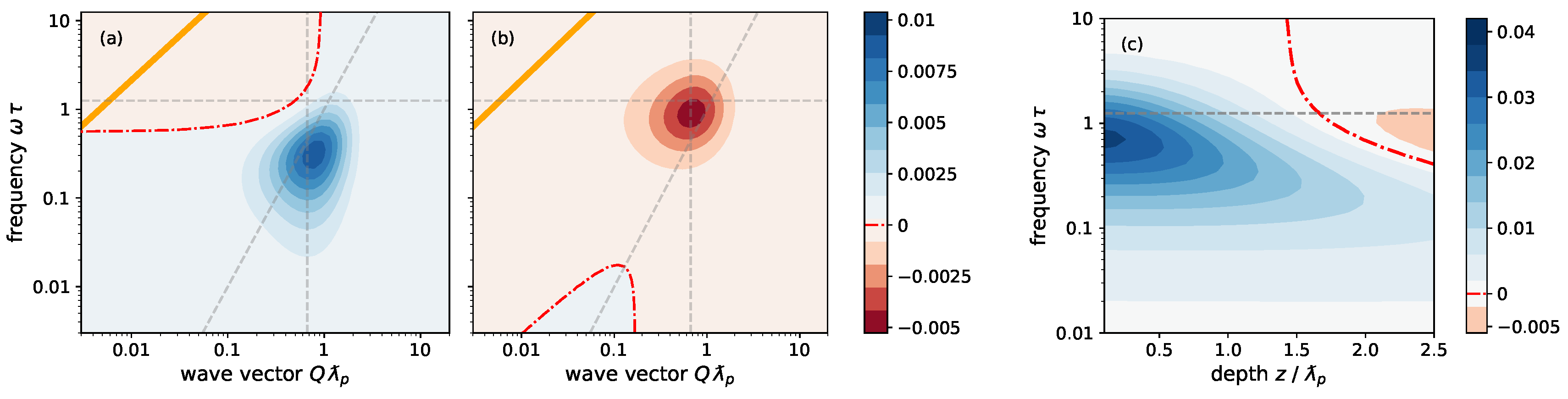
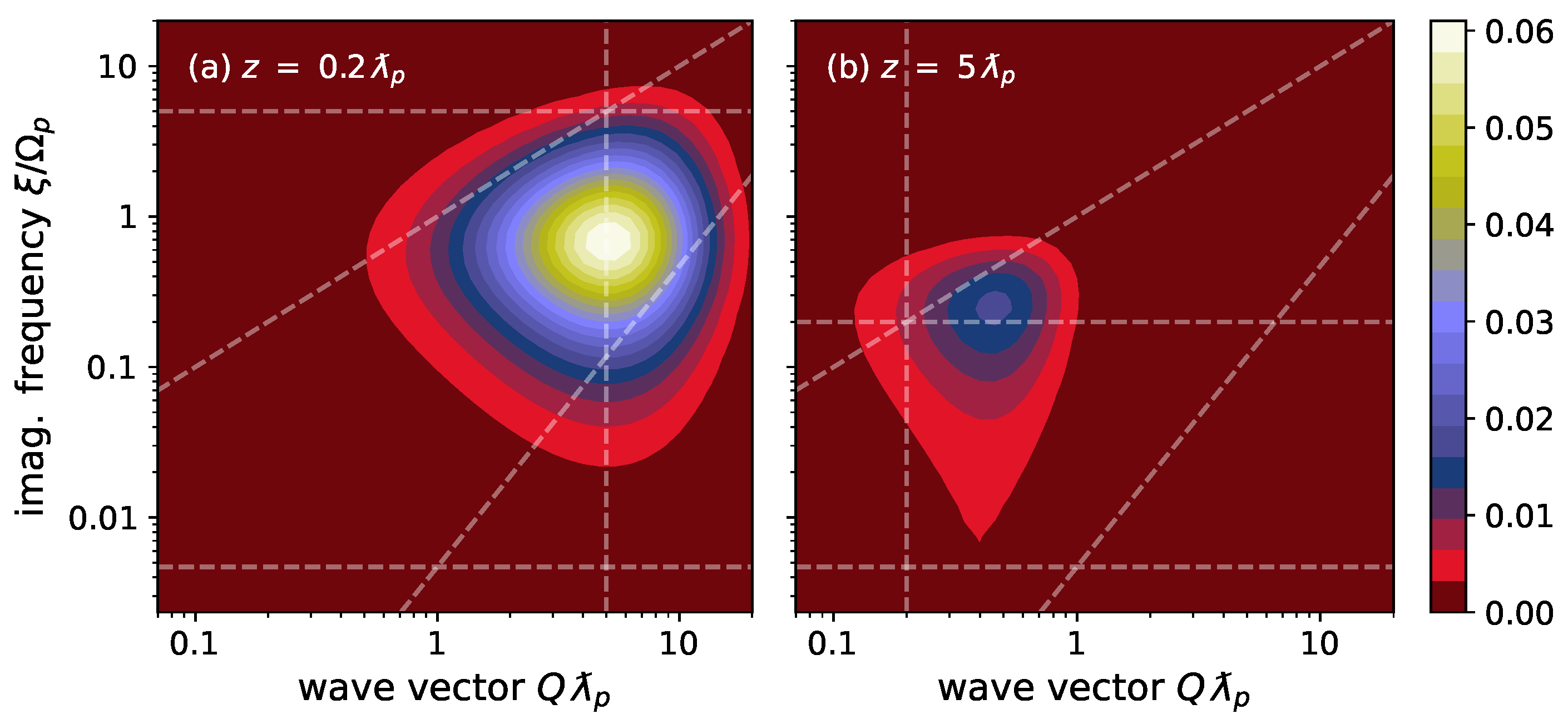
3.1. General Features

A net force appears only due to the reflection from the surface at $z=0$, as expected from broken rotational symmetry. Similar to the Casimir effect, the Lorentz force contains a specific quantum contribution that is UV-dominated, since $coth\frac{1}{2}\beta \omega \to 1$ at high frequencies. In practice, the UV transparency of the material makes this contribution finite. Indeed, from the sum of the two Fresnel amplitudes,

$$r_s+r_p=\frac{2vq(\epsilon -{\epsilon }_0)}{(\epsilon v+{\epsilon }_{0}q)(q+v)},$$

(15)

it appears explicitly that the integrand decays sufficiently fast at high frequencies. This is illustrated in Figure 1 and Figure 2 where the integrand of Equation (14) is plotted.

In the zero-temperature limit, it is expedient to shift the frequency integration to the imaginary axis, $\omega =\mathrm{i}\xi$. In this representation, relatively large frequencies and wave vectors are exponentially damped by the factor ${\mathrm{e}}^{2\mathrm{i}qz}\approx exp[-2(z/c)\sqrt{{\mathsf{\Omega }}_p^2+{\xi }^2+c^2{Q}^2}]$ (this approximation assumes $\xi \gg 1/\tau$). An approximate estimate of the double integral yields a scaling of the average Lorentz force density according to

$$T=0:f(z,0)\sim \frac{\hslash {\mathsf{\Omega }}_p}{{ƛ}_p{z}^3},$$

(16)

where ${ƛ}_p=c/{\mathsf{\Omega }}_p$ represents the plasma wavelength.

We expect both the plasma and the Drude model to give comparable contributions, unless distances larger than $c\tau \gg {ƛ}_p$ are considered. In addition, for frequencies in the visible range and above, it is mandatory to take into account deviations from the Drude (or plasma) models, using, e.g., tabulated optical data [28]. A more detailed discussion is left for future studies.

Deep in the bulk, $z\to +\infty$, the exponential ${\mathrm{e}}^{2\mathrm{i}qz}$ makes the force vanish. Since the medium wave vector q in Equation (14) is complex, one may expect an oscillatory behavior. The exponential ${\mathrm{e}}^{2iqz}$ becomes approximately real deeply below the light cone ($Q\gg \omega /c$). The typical long-range behaviour in the infrared is $q\approx (1+\mathrm{i})/\delta$ with the skin depth ${\delta }^2=2/\left({\mu }_0{\sigma }_0\omega \right)$. This corresponds to the diffusive propagation of magnetic fields in a conducting medium.

The limit $z\to 0$ is beyond the local (Drude or plasma) model because $r_p$ tends towards a constant at large Q, destroying convergence. This is eliminated when using a nonlocal ($\mathbf{q}$-dependent) conductivity whose magnitude drops for short-wavelength fields. The leading-order behaviour in the local approximation is discussed in Section 3.2 just below.

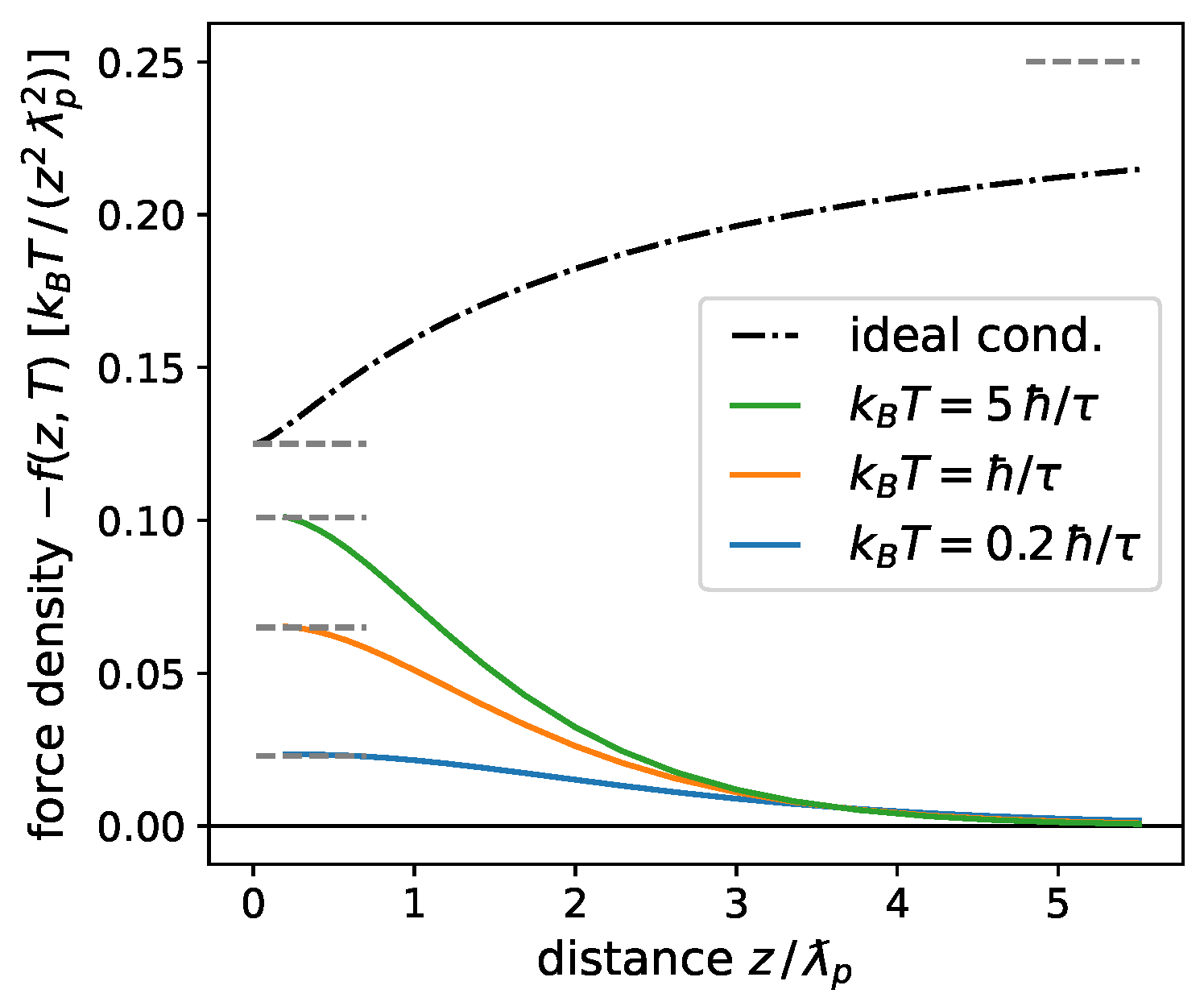
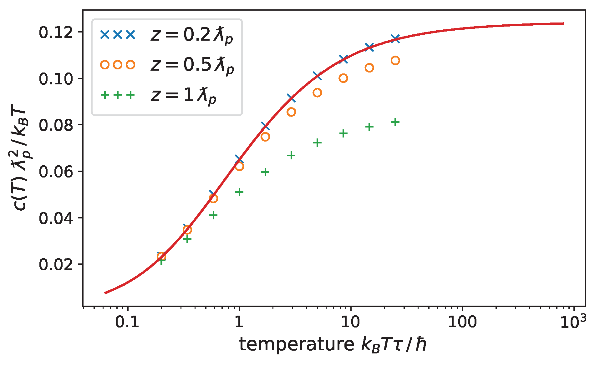
3.2. Thermal Hall Force

In what follows, the quantum contribution is subtracted, $coth(\hslash \omega /2k_{B}T)-1=2\overline{n}(\omega /T)$, so that the thermal component of the Lorentz force is proportional to the Bose–Einstein distribution $\overline{n}(\omega /T)$. The latter is dominated by frequencies with $\hslash \omega \lesssim k_{B}T$ (mid infrared and below, see Figure 2c). The plots in Figure 2a,b illustrate that the integrand of Equation (14) in the $(Q,\omega )$-plane (Figure 2a) would change sign if only the term due to field fluctuations were kept (Figure 2b).

Note that in the plasma model, where the conductivity is entirely imaginary, the integrand is nonzero only above the light cone ($\omega >cQ$) and approximately above the plasma frequency ${\mathsf{\Omega }}_p$. Otherwise, the medium wave vector q is entirely imaginary, and the reflection coefficients $r_s$ and $r_p$ turn out to be real. This highly suppresses the thermal contribution to the average Lorentz force, since for typical temperatures, one has $\hslash {\mathsf{\Omega }}_p\gg k_{B}T$. It is therefore instructive to evaluate the contribution from the singular DC conductivity of Equation (10). In calculations along imaginary frequencies, using a generalised plasma model, this term generates a permittivity $\epsilon \left(\mathrm{i}\xi \right)\sim {\mathsf{\Omega }}_p^2/{\xi }^2$, either by inserting Equation (10) into Kramers–Kronig relations or, more cautiously, by first isolating the zero-frequency pole [29,30]. However, a physical interpretation in terms of current fluctuations for superconductors is not clear enough. Fields penetrate into a superconducting medium down to approximately the same depth (the plasma wavelength ${ƛ}_p$) as the layer where the thermal Lorentz force is nonzero, see Figure 3. However, one would expect from the Meißner effect that in the bulk of a sample, there are neither static currents nor magnetic fields. In Ref. [31], Francesco Intravaia and the present author suggested to interpret the fluctuation electrodynamics of a medium with Equation (10) in terms of an “ideal conductor” model. Its bulk is filled with “frozen currents” and concomitant magnetic field loops. Inserting the conductivity (10) into Equation (14), one obtains for the thermal Lorentz force the expression

$$\left(\mathrm{ideal}\mathrm{conductor}\right)\Delta f(z,T)=-\frac{k_{B}T}{{ƛ}_p^2}\underset{0}{\overset{\infty }{\int }}\mathrm{d}Q{\mathrm{e}}^{-2Qz}\frac{Q\kappa }{\kappa +Q}+\exp .\mathrm{small}\mathrm{terms}$$

(17)

with ${\kappa }^2={({\mathsf{\Omega }}_p/c)}^2+Q^2$. The integral here has the asymptotic form $1/\left(8z^2\right)$ (or $1/\left(4z^2\right)$) for $z\ll {ƛ}_p$ (for $z\gg {ƛ}_p$), the same scaling as the Coulomb force due to image charges. The exponentially small terms arise from frequencies $\hslash \omega \gtrsim \hslash {\mathsf{\Omega }}_p\gg k_{B}T$. The resulting force is shown as dashed-dotted lines in Figure 3.

In good metallic conductors, the reflection coefficients are dominated by $|r_p|\approx 1$, while $r_s\approx -\frac{1}{4}(\epsilon -1){(\omega /cQ)}^2\to 0$ for $Q\gg \left|\epsilon \right|\omega /c,\omega /c$ (evanescent waves). This allows for an approximate evaluation of the Q-integral in Equation (14). In the leading order, $r_s$ is dropped, and one obtains again the scaling law $f\sim -1/z^2$. It has been checked that this captures well the short-distance behaviour of the force density, $f(z,T)\approx -c_2\left(T\right)/z^2$ with a prefactor given by

$$\begin{array}{cc}\hfill c_2\left(T\right)& \approx \frac{\hslash {\mu }_0{\sigma }_0}{4\pi }\underset{0}{\overset{\infty }{\int }}\mathrm{d}\omega \frac{\omega \overline{n}(\omega /T)}{1+{\omega }^2{\tau }^2}\hfill \\ \hfill & =\frac{k_{B}T}{8\pi {ƛ}_p^2}\left(\beta log\frac{\beta }{2\pi }-\pi -\beta \psi (\beta /2\pi )\right).\hfill \end{array}$$

(18)

Here, $\beta =\hslash /\left(k_{B}T\tau \right)$ and $\psi (·)$ is the digamma function. Recall that $\tau$ is the scattering time in the Drude conductivity, and $\overline{n}(\omega /T)$ the Bose–Einstein distribution. This expression is shown in Figure 4 after dividing out the scale factor $k_{B}T/{ƛ}_p^2$: one observes only quite minor dynamics, even though the product $k_{B}T\tau /\hslash$ varies over three orders of magnitude. The agreement with the full numerical integration is particularly good at the short distance $z=0.2{ƛ}_p$.

The distance dependence at a fixed temperature can be found from Figure 3 where the combination $-f(z,T)z^2/\left(k_{B}T\right)$ is shown. The force decays into the bulk with strongly damped oscillations, of which there remains only a crossing of the curves for different temperatures at a depth $z\approx 3.5{ƛ}_p$. Beyond this depth, the linear scaling with temperature becomes exact. The rectified Lorentz force is thus restricted to a few plasma penetration depths, typically about $100\mathrm{nm}$. The ideal conductor also gives a scaling linear in T, but the weak modifications relative to the $1/z^2$ power law display the opposite trend.

3.3. Physical Consequences

Among the physical consequences suggested by these calculations, Section 1 mentioned a temperature-dependent shift $\Delta \varphi \left(T\right)$ in the work function of a metal. Indeed, the Lorentz force is pulling charges towards the surface. To calculate the corresponding energy gain, one needs to regularise the $1/z^2$ divergence as $z\to 0$. This is physically achieved by adopting a non-local dielectric function (spatial dispersion), as discussed in Refs. [26,32,33]. A characteristic length scale related to the compressibility of the electron gas is the Debye screening length, ${\mathit{\ell }}_D=v_F/{\mathsf{\Omega }}_p$, where $v_F$ is typically of the order of the Fermi velocity.

If one integrates the Lorentz force density from $z=\infty$ down to a cutoff at $z={\mathit{\ell }}_D$ and divides by the equilibrium carrier density $n_0$, the following estimate is obtained

$$\Delta \varphi \left(T\right)\approx -\frac{c_2\left(T\right)}{n_0{\mathit{\ell }}_D}\approx -0.06k_{B}T\frac{e^2}{{\epsilon }_0\hslash c}\frac{\hslash /{ƛ}_p}{m{v}_F}.$$

(19)

Both ratios on the right-hand side of Equation (19) are less than unity: the first ratio is $4\pi /137\approx 0.0917$, and for gold, the second ratio results to $\approx 0.00380$. However, a Kelvin probe locked to a periodic temperature modulation may prove to be sufficiently sensitive.

A complementary phenomenon is the induced subsurface space charge that screens the thermal Lorentz force, restoring electro-chemical equilibrium. From the Coulomb law, its cumulative density $\Delta Q/A$ per unit area is of the order of

$$\frac{\Delta Q}{A}\approx \frac{{\epsilon }_0}{e{n}_0}\underset{z\to {\mathit{\ell }}_D}{lim}f\left(z\right)\approx -0.06\frac{e}{{ƛ}_p^2}\frac{k_{B}T}{m{v}_F^2}.$$

(20)

This is again, as just above, a quite small charge, barely an elementary charge per square micron for gold. If this charge shows fluctuations in the MHz frequency band, however, these may be detectable with miniaturised ion traps because the corresponding fluctuations in the Coulomb force work against the laser cooling of the ion to its motional ground state [34].

4. Conclusions

In this paper, a thermal Hall effect has been explored that arises from the correlation between current density and magnetic field in a conducting medium at finite temperature. It turns out that in a thin layer below the material surface (its thickness being comparable to the Meißner penetration depth, ${ƛ}_p$), the Lorentz force density, averaged over thermal fluctuations, is nonzero and points towards the surface, similar to the interaction with image charges. It has been found that a Drude model gives a distinct prediction compared to the so-called plasma model because the corresponding force spectra have opposite signs (see Figure 2a,b). The thermal Hall voltage is relatively small, however.

The next step could be the regularisation on short-length scales, using a spatially dispersive permittivity and suitable boundary conditions. Another interesting perspective is the fluctuation spectrum of the Lorentz force around its thermal average that arises from fourth-order correlations of Rytov currents. This may provide an alternative, physical picture for the unusual electric field fluctuations observed in ion traps (anomalous heating) that are often attributed to surface contaminations [34].

References

1. Uhlig, R.P.; Zec, M.; Brauer, H.; Thess, A. Lorentz force eddy current testing: A prototype model. J. Nondestruct. Eval. 2012, 31, 357–372. [Google Scholar] [CrossRef]
2. Li, C.; Liu, R.; Dai, S.; Zhang, N.; Wang, X. Vector-based eddy-current testing method. Appl. Sci. 2018, 8, 2289. [Google Scholar] [CrossRef]
3. Alkhalil, S.; Kolesnikov, Y.; Thess, A. Lorentz force sigmometry: A novel technique for measuring the electrical conductivity of solid and liquid metals. Meas. Sci. Technol. 2015, 26, 115605. [Google Scholar] [CrossRef]
4. Bloembergen, N.; Chang, R.K.; Jha, S.S.; Lee, C.H. Optical second-harmonic generation in reflection from media with inversion symmetry. Phys. Rev. 1969, 178, 1528. [Google Scholar] [CrossRef]
5. Sipe, J.E.; So, V.C.Y.; Fukui, M.; Stegeman, G.I. Analysis of second-harmonic generation at metal surfaces. Phys. Rev. B 1980, 21, 4389–4402. [Google Scholar] [CrossRef]
6. Renger, J.; Quidant, R.; van Hulst, N.; Palomba, S.; Novotny, L. Free-space excitation of propagating surface plasmon polaritons by nonlinear four-wave mixing. Phys. Rev. Lett. 2009, 103, 266802. [Google Scholar] [CrossRef] [PubMed]
7. Renger, J.; Quidant, R.; van Hulst, N.; Novotny, L. Surface-enhanced nonlinear four-wave mixing. Phys. Rev. Lett. 2010, 104, 046803. [Google Scholar] [CrossRef]
8. Hille, A.; Moeferdt, M.; Wolff, C.; Matyssek, C.; Rodríguez-Oliveros, R.; Prohm, C.; Niegemann, J.; Grafström, S.; Eng, L.M.; Busch, K. Second harmonic generation from metal nano-particle resonators: Numerical analysis on the basis of the hydrodynamic Drude model. J. Phys. Chem. C 2016, 120, 1163–1169. [Google Scholar] [CrossRef]
9. Kadlec, F.; Kužel, P.; Coutaz, J.-L. Optical rectification at metal surfaces. Opt. Lett. 2004, 29, 2674–2676. [Google Scholar] [CrossRef]
10. Hoffmann, M.C.; Fülöp, J.A. Intense ultrashort terahertz pulses: Generation and applications. J. Phys. D Appl. Phys. 2011, 44, 083001. [Google Scholar] [CrossRef]
11. Trinh, M.T.; Smail, G.; Makhal, K.; Yang, D.S.; Kim, J.; Rand, S.C. Observation of magneto-electric rectification at non-relativistic intensities. Nat. Commun. 2020, 11, 5296. [Google Scholar] [CrossRef] [PubMed]
12. Craig, R.A. Dynamic contributions to the surface energy of simple metals. Phys. Rev. B 1972, 6, 1134–1142. [Google Scholar] [CrossRef]
13. Morgenstern Horing, N.J.; Kamen, E.; Gumbs, G. Surface correlation energy and the hydrodynamic model of dynamic, nonlocal bounded plasma response. Phys. Rev. B 1985, 31, 8269–8272. [Google Scholar] [CrossRef] [PubMed]
14. Barton, G. On the surface energy of metals according to the hydrodynamic model with spatial dispersion. J. Phys. C Sol. State Phys. 1986, 19, 975–980. [Google Scholar] [CrossRef]
15. Prange, R.E.; Kadanoff, L.P. Transport theory for electron–phonon interactions in metals. Phys. Rev. 1964, 134, A566–A580. [Google Scholar] [CrossRef]
16. Pudell, J.; Maznev, A.; Herzog, M.; Kronseder, M.; Back, C.; Malinowski, G.; von Reppert, A.; Bargheer, M. Layer specific observation of slow thermal equilibration in ultrathin metallic nanostructures by femtosecond X-ray diffraction. Nat. Commun. 2018, 9, 3335. [Google Scholar] [CrossRef]
17. Bresson, P.; Bryche, J.F.; Besbes, M.; Moreau, J.; Karsenti, P.L.; Charette, P.G.; Morris, D.; Canva, M. Improved two-temperature modeling of ultrafast thermal and optical phenomena in continuous and nanostructured metal films. Phys. Rev. B 2020, 102, 155127. [Google Scholar] [CrossRef]
18. Rytov, S.M.; Kravtsov, Y.A.; Tatarskii, V.I. Principles of Statistical Radiophysics. Volume 3: Elements of Random Fields; Springer: Berlin/Heidelberg, Germany, 1989. [Google Scholar]
19. Griniasty, I.; Leonhardt, U. Casimir stress inside planar materials. Phys. Rev. A 2017, 96, 032123. [Google Scholar] [CrossRef]
20. Klimchitskaya, G.L.; Mostepanenko, V.M.; Svetovoy, V.B. Experimentum crucis for electromagnetic response of metals to evanescent waves and the Casimir puzzle. Universe 2022, 8, 574. [Google Scholar] [CrossRef]
21. Klimchitskaya, G.L.; Mostepanenko, V.M.; Svetovoy, V.B. Probing the response of metals to low-frequency s-polarized evanescent fields. Europhys. Lett. 2022, 139, 66001. [Google Scholar] [CrossRef]
22. Henkel, C. Nano-scale thermal transfer—An invitation to fluctuation electrodynamics. Z. Naturforsch. A 2017, 72, 99–108. [Google Scholar] [CrossRef]
23. Klimchitskaya, G.L.; Mostepanenko, V.M. Recent measurements of the Casimir force: Comparison between experiment and theory. Mod. Phys. Lett. A 2020, 35, 2040007. [Google Scholar] [CrossRef]
24. Conti, S.; Vignale, G. Elasticity of an electron liquid. Phys. Rev. B 1999, 60, 7966–7980. [Google Scholar] [CrossRef]
25. Hannemann, M.; Wegner, G.; Henkel, C. No-slip boundary conditions for electron hydrodynamics and the thermal Casimir pressure. Universe 2021, 7, 108. [Google Scholar] [CrossRef]
26. Dressel, M.; Grüner, G. Electrodynamics of Solids–Optical Properties of Electrons in Matter; Cambridge University Press: Cambridge, UK, 2002. [Google Scholar] [CrossRef]
27. Berlinsky, A.J.; Kallin, C.; Rose, G.; Shi, A.C. Two-fluid interpretation of the conductivity of clean BCS superconductors. Phys. Rev. B 1993, 48, 4074–4079. [Google Scholar] [CrossRef] [PubMed]
28. Klimchitskaya, G.L.; Mohideen, U.; Mostepanenko, V.M. The Casimir force between real materials: Experiment and theory. Rev. Mod. Phys. 2009, 81, 1827–1885. [Google Scholar] [CrossRef]
29. Klimchitskaya, G.L.; Mohideen, U.; Mostepanenko, V.M. Kramers-Kronig relations for plasma-like permittivities and the Casimir force. J. Phys. A 2007, 40, F339–F346. [Google Scholar] [CrossRef]
30. Levine, Z.H.; Cockayne, E. The pole term in linear response theory: An example from the transverse response of the electron gas. J. Res. Natl. Inst. Stand. Technol. 2008, 113, 299–304. [Google Scholar] [CrossRef] [PubMed]
31. Henkel, C.; Intravaia, F. On the Casimir entropy between ‘perfect crystals’. Int. J. Mod. Phys. A 2010, 25, 2328–2336. [Google Scholar] [CrossRef]
32. Sernelius, B.E. Effects of spatial dispersion on electromagnetic surface modes and on modes associated with a gap between two half spaces. Phys. Rev. B 2005, 71, 235114. [Google Scholar] [CrossRef]
33. Svetovoy, V.B.; Esquivel, R. The Casimir free energy in high- and low-temperature limits. J. Phys. A 2006, 39, 6777–6784. [Google Scholar] [CrossRef]
34. Brownnutt, M.; Kumph, M.; Rabl, P.; Blatt, R. Ion-trap measurements of electric-field noise near surfaces. Rev. Mod. Phys. 2015, 87, 1419–1482. [Google Scholar] [CrossRef]
35. Sipe, J.E. New Green-function formalism for surface optics. J. Opt. Soc. Am. B 1987, 4, 481–489. [Google Scholar] [CrossRef]
36. Agarwal, G.S. Quantum electrodynamics in the presence of dielectrics and conductors. I. Electromagnetic-field response functions and black-body fluctuations in finite geometries. Phys. Rev. A 1975, 11, 230–242. [Google Scholar] [CrossRef]
37. Lifshitz, E.M.; Pitaevskii, L.P. Statistical Physics. Part 2: Theory of the Condensed State; Butterworth–Heinemann Ltd./Elsevier Ltd.: Oxford, UK, 1980. [Google Scholar] [CrossRef]
38. Buhmann, S.Y. Dispersion Forces II. Many-Body Effects, Excited Atoms, Finite Temperature and Quantum Friction; Springer: Berlin/Heidelberg, Germany, 2012. [Google Scholar] [CrossRef]
Figure 1. Integrand of the average Lorentz force due to quantum fluctuations ( T = 0 , arbitrary units) for (a) short and (b) large distances, as indicated. A Wick rotation to imaginary frequencies ξ has been applied. Parameters: plasma frequency Ω p 210 / τ (typical for Au). The dashed lines in (a,b) mark the values ξ = c / z , ξ = c Q (light cone), ξ = Q 2 / ( μ 0 σ 0 ) (magnetic diffusion), ξ = 1 / τ , and Q = 1 / z . To reduce the dynamics of the data points, the integrand has been multiplied by z 3 . See text for more details.
Physics 06 00037 g001
Figure 2. Spectrum of the thermal Lorentz force density (arbitrary units, real frequencies): (a,b) integrand of Equation (14), with the T = 0 contribution subtracted and (b) with only the imaginary part of the conductivity kept (similar to the plasma model); (c) the spectrum f ( z , ω ) before evaluating the ω -integral. Sign changes occur at the red dashed-dotted lines. Parameters: temperature k B T = 1.25 / τ , plasma frequency Ω p 210 / τ (as in Figure 1), distance z = 1.5 ƛ p in (a,b). The dashed lines in (a,b) mark the values Q = 1 / z , ω = k B T , and in solid orange the light cone ω = c Q . The dashed line in (c) indicates ω = k B T . To reduce the dynamics of the data points in (c), the force has been multiplied by z 2 .
Physics 06 00037 g002
Figure 3. Distance dependence of the DC force density, normalised to T / z 2 and with flipped sign, for different temperatures, calculated for an ideal conductor (17) (black dashed-dotted curve) and a Drude conductor with finite damping time τ (colour curves). The straight dashed gray lines show the short-distance and large-distance limits of Equation (17) and the short-distance limit of Equation (18). The parameters are as in Figure 2: for typical conductors such as Au, the parameters correspond to / τ 400 K and ƛ p = c / Ω p 20 nm .
Physics 06 00037 g003
Figure 4. Temperature dependence of the amplitude c 2 ( T ) of the rectified Lorentz force density f c 2 ( T ) / z 2 at short distances, normalised to k B T / ƛ p 2 , calculated using Equation (18) (solid line) and with the numerical integration of Equation (14) with the T = 0 contribution subtracted (symbols). Material parameters as in Figure 2. Here, τ is not temperature-dependent.
Physics 06 00037 g004
Disclaimer/Publisher’s Note: The statements, opinions and data contained in all publications are solely those of the individual author(s) and contributor(s) and not of MDPI and/or the editor(s). MDPI and/or the editor(s) disclaim responsibility for any injury to people or property resulting from any ideas, methods, instructions or products referred to in the content.