Ultrafast Resonant Photon Emission from a Molecule Driven by a Strong Coherent Field in Terms of Complex Spectral Analysis

Abstract

In this study, we investigate the time–frequency-resolved resonant photon emission from a molecular vibrational oscillator driven by a monochromatic coherent external field. Using the complex spectral analysis of the Liouvillian, which integrates irreversible dissipative phenomena into quantum theory, we elucidate the fundamental processes of photon emission. Indeed, our analytical approach successfully decomposes the emission spectrum into two intrinsic contributions: one from a resonance eigenmode and another from continuous eigenmodes. These components are responsible for incoherent luminescence and coherent scattering photon emission processes, respectively. Our results show that while spontaneous emission dominates in the early stages of the emission process, coherent scattering gradually becomes more pronounced with time. Furthermore, destructive quantum interference between the two components plays a key role in determining the overall shape of the emission spectrum.

1. Introduction

Spontaneous emission from an excited atom is a fundamental process in light–matter interactions. It is an irreversible dissipative process due to quantum fluctuations of the electromagnetic field and energetic resonance between the atomic excited states and the radiation field. The Weisskopf–Wigner theory explains the Lorentzian-shaped spontaneous emission spectrum of an excited atom with use of the solutions of the Heisenberg equation, where the dissipation effect of an atomic excitation is taken into account phenomenologically by introducing a decay constant [1,2]. This theory assumes that the atom is in the excited state as the initial state and does not address how the excitation process affects the photon emission process. In contrast, Yutaka Toyozawa and collaborators studied a correlation of excitation and photon emission processes in a resonant light emission, treating it as a sequential coherent quantum process. They revealed that two different types of photon emission processes coexist: coherent light scattering and incoherent luminescence [3,4,5]. While in the former the emitted photon energy is correlated with the incident light energy, in the latter, the correlation disappears due to the dissipation effect.

Recent progress in the development of strong laser sources allows us to explore various new types of light emission from light-driven materials [6,7,8,9,10], such as high harmonic generation and high-order sideband generation [11,12,13,14,15,16,17]. These are often considered as high-order nonlinear optical phenomena, where coherently driven electronic systems give rise to substantial electronic currents or polarizations that subsequently act as sources of classical radiation [15,18,19,20]. This leads to fundamental questions: how is quantum mechanical spontaneous emission in a weak excitation related to coherent classical radiation in a strong coherent driving situation, and how can coherent scattering and incoherent luminescence coexist? Answering these questions requires a quantum mechanical treatment of light emission processes, considering the whole system of light and matter. Although several studies have analyzed radiation processes quantum mechanically, they have been largely limited to the lower-order perturbation regime [21,22,23].

Even with a higher-order perturbation method, a fundamental challenge remains: how to describe dissipative spontaneous emission in a way that is consistent with quantum theory. Traditional approaches yield only time-reversible unitary evolution from hermitian Hamiltonian dynamics. To fill this gap, several extensions of quantum theory have been proposed to include irreversible dissipation [24,25,26,27,28,29,30]. Among these, the contributions by Ilya Prigogine and collaborators [25,28,31] and by Arno Bohm and collaborators [24,30,32] are notable; they extend the vector space beyond the conventional Hilbert space to the rigged Hilbert space, or the Gel’fand triplet [33]. In this extended framework, called complex spectral analysis, the time evolution generators—specifically, Hamiltonian and Liouvillian—can have complex eigenvalues, thus allowing irreversible processes.

Using complex spectral analysis, we have studied optical dissipative processes to elucidate the role of resonance states characterized by complex eigenvalues [34,35]. Our recent investigations used this analysis in conjunction with Floquet theory to study high-order sideband generation in a coherently driven two-level system [36], revealing both transient and stationary spectral profiles. Through this analysis, we distinguished the resonant state contributions in the photon emission spectrum from the dressed continuous state contributions and identified instances of destructive interference between the two. These studies assumed an initial excited state for the two-level system and a modification of its energy levels by the driving field. However, this initial condition precludes the clarification of the energy correlation between incident and emitted light and, thus, hinders the study of the interplay between scattering and luminescence under strong driving fields.

In this paper, we present a theoretical formulation for the resonant photon emission of a harmonic oscillator driven by a strong coherent field. Our approach uniquely considers the quantized radiation field as an integral part of the whole system. Unlike in the previous studies [15,18,19,20], we focus here on the irreversible spontaneous photon emission process under a strong driving field, which requires an extension beyond conventional quantum theory restricted to Hilbert space. We address this by solving the complex eigenvalue problem of the Liouvillian, the generator of the Heisenberg equation, to elucidate the resonance mode responsible for the irreversible spontaneous emission that manifests as incoherent luminescence.

In terms of complex spectral analysis, our results reveal the physical origins of resonance photon emission under strong coherent drive. The solution we provide is exact, eliminating ambiguities in the physical interpretation of the spectrum. We present the time–frequency-resolved photon emission spectrum and show that incoherent luminescence contributions can exist even under strong coherent drive. Furthermore, our results emphasize the important role of coherent photon emission at the molecular resonance. In particular, destructive interference plays a key role during the initial stages of photon emission, profoundly influencing the build-up of the spectral structure.

The structure of this paper is organized as follows. In Section 2, we introduce our model system and describe the Liouvillian, which serves as the generator for the time evolution of the quantum dynamical variables. Section 3 details the derivation of complex eigenmodes and presents the solution of the Heisenberg equation. The calculated results, including molecular excitation and the resonant photon emission spectrum, are discussed in Section 4. We conclude in Section 5 with a summary of our results and further discussions. We introduce the symplectic structure of the present system in Appendix A, derive the effective Liouvillian in Appendix B, and obtain the complex eigenmode operators in Appendix C. The solution of the Heisenberg equations and the spectral expressions are given in Appendix D.

2. Model

In this paper, we study the photon emission from a polarizable diatomic molecule driven by a time-dependent strong coherent driving electric field, where the stretching vibrational mode is described by a harmonic oscillator interacting with the time-dependent external field. The Hamiltonian operator for this system is then given by

$$\begin{array}{cc}\widehat{H}(t)\hfill & =\widehat{H}+\widehat{W}(t),\hspace{1em}\hspace{1em}\hspace{1em}\hspace{1em}\hspace{1em}\hspace{1em}\hspace{1em}\hspace{1em}\hspace{1em}\hspace{1em}\hspace{1em}\hspace{1em}\hspace{1em}\hspace{1em}\hspace{1em}\hspace{1em}\hspace{1em}\hspace{1em}\hfill \end{array}$$

(1)

$$\begin{array}{cc}\hfill \widehat{H}& \hfill ={\omega }_0\left({\widehat{a}}^{†}\widehat{a}+\frac{1}{2}\right)+\int dk{\omega }_k\left({\widehat{b}}_k^{†}{\widehat{b}}_k+\frac{1}{2}\right)+\int dk{g}_k({\widehat{a}}^{†}{\widehat{b}}_k+\widehat{a}{\widehat{b}}_k^{†}),\end{array}$$

(2)

$$\begin{array}{cc}\widehat{W}(t)\hfill & =f(t)({\widehat{a}}^{†}+\widehat{a}),\hspace{1em}\hspace{1em}\hspace{1em}\hspace{1em}\hspace{1em}\hspace{1em}\hspace{1em}\hspace{1em}\hspace{1em}\hspace{1em}\hspace{1em}\hspace{1em}\hspace{1em}\hspace{1em}\hspace{1em}\hspace{1em}\hspace{1em}\hspace{1em}\hfill \end{array}$$

(3)

where the hat denotes the operator, $\widehat{a}$ (${\widehat{a}}^{†}$) is the annihilation (creation) boson operator for the harmonic oscillator representing the stretching vibration of a diatomic molecule with natural frequency ${\omega }_0$. In this paper, we set the reduced Planck constant, $\hslash =1$. In what follows, we refer to this oscillator as the “molecular oscillator” or just the “molecule”. The emitted radiation field is treated quantum mechanically, as described by the second term in Equation (2), where ${\widehat{b}}_k$ (${\widehat{b}}_k^{†}$) are the annihilation and creation boson operators for the radiation field with wavenumber k and frequency ${\omega }_k$. Specific wavenumber dependencies of these parameters are used in the numerical calculation described in Section 4. The third term in Equation (2) represents the interaction between the molecular oscillator and the radiation field with the real coupling constant $g_k$. The Hamiltonian $\widehat{H}$, known as the Friedrichs model, has been used extensively to describe quantum mechanically an irreversible spontaneous emission process from an excited atom [2,25,37]. The interaction of the molecular oscillator with an external time-dependent driving field is represented by $\widehat{W}(t)$ (3).

Here, we define a set of Heisenberg operators as a vector:

$$\begin{array}{c}\hfill \widehat{\xi }(t):={(\widehat{a}(t),\left\{{\widehat{b}}_k(t)\right\};{\widehat{a}}^{†}(t),\left\{{\widehat{b}}_k^{†}(t)\right\})}^T,\end{array}$$

(4)

where $\left\{{\widehat{b}}_k(t)\right\}$ and $\left\{{\widehat{b}}_k^{†}(t)\right\}$ are infinite dimensional row vectors of annihilation and creation operators, respectively, for continuous k variables, and T is the transpose. We solve the Heisenberg equation,

$$i{\partial }_t\widehat{\xi }(t)=\widehat{\mathcal{L}}(t)\widehat{\xi }(t)=\widehat{\mathcal{L}}\widehat{\xi }(t)+\mathit{F}(t),$$

(5)

with the initial condition

$$\begin{array}{c}\hfill \widehat{\xi }(0)=\widehat{\xi }={(\widehat{a},\left\{{\widehat{b}}_k\right\};{\widehat{a}}^{†},\left\{{\widehat{b}}_k^{†}\right\})}^T.\end{array}$$

(6)

In Equation (5), $\widehat{\mathcal{L}}(t)$ and $\widehat{\mathcal{L}}$ denote the Liouvillian superoperator defined by the commutation relation with $\widehat{H}(t)$ and $\widehat{H}$, respectively:

$$\begin{array}{c}\hfill \widehat{\mathcal{L}}(t)·\equiv [\widehat{H}(t),·]=[\widehat{H}+\widehat{W}(t),·],\widehat{\mathcal{L}}·\equiv [\widehat{H},·].\end{array}$$

(7)

The Liouvillian superoperator $\widehat{\mathcal{L}}$ is represented by a block diagonal matrix for the annihilation operator set $(\widehat{a},\left\{{\widehat{b}}_k\right\})$ and the creation operator set $({\widehat{a}}^{†},\left\{{\widehat{b}}_k^{†}\right\})$:

$$\mathit{L}=\left(\begin{array}{cc}{\mathit{L}}_{\mathrm{B}}& 0\\ 0& -{\mathit{L}}_B\end{array}\right),$$

(8)

where the submatrix ${\mathit{L}}_{\mathrm{B}}$ is represented by a Hermitian matrix,

$${\mathit{L}}_{\mathrm{B}}\equiv \left(\begin{array}{cc}{\omega }_0& \left\{g_k\right\}\\ {\left\{g_k\right\}}^T& \mathrm{diag}(\left\{{\omega }_k\right\})\end{array}\right)={\mathit{L}}_{\mathrm{B}}^T.$$

(9)

The last term of Equation (5) is due to the interaction of the molecule with the driving field represented by $\mathit{F}(t):={(f(t),\left\{0_k\right\},-f(t),\left\{0_k\right\})}^T$.

To solve the Heisenberg Equation (5), we first find invertible transformation matrices $\tilde{\mathsf{\Phi }}$ and $\mathsf{\Phi }$ to diagonalize the time-independent Liouvillian $\mathit{L}$ given by Equation (8):

$$\begin{array}{c}\hfill \tilde{\mathsf{\Phi }}\mathit{L}\mathsf{\Phi }=\mathit{Z}.\end{array}$$

(10)

Since the total Liouvillian takes the block diagonal form Equation (8), we can write

$$\begin{array}{c}\hfill \tilde{\mathsf{\Phi }}=\left(\begin{array}{cc}{\tilde{\mathsf{\Phi }}}_{\mathrm{B}}& 0\\ 0& {\tilde{\mathsf{\Phi }}}_{\mathrm{B}}^{★}\end{array}\right),\mathsf{\Phi }=\left(\begin{array}{cc}{\mathsf{\Phi }}_{\mathrm{B}}& 0\\ 0& {\mathsf{\Phi }}_{\mathrm{B}}^{★}\end{array}\right),\mathit{Z}=\left(\begin{array}{cc}{\mathit{Z}}_{\mathrm{B}}& 0\\ 0& -{\mathit{Z}}_{\mathrm{B}}\end{array}\right),\end{array}$$

(11)

so that

$$\begin{array}{c}\hfill \tilde{\mathsf{\Phi }}\mathsf{\Phi }=\mathit{I}\end{array}$$

(12)

and

$$\begin{array}{c}\hfill {\mathit{Z}}_{\mathrm{B}}=\mathrm{diag}(z_a,\left\{z_k\right\}),\end{array}$$

(13)

where ★-transformation is defined in Equations (A10) and (A11). Below, we show how to construct $\tilde{\mathsf{\Phi }}$, $\mathsf{\Phi }$ and obtain $\mathit{Z}$ in Appendices Appendix A and Appendix C in terms of the Brillouin–Wigner–Feshbach projection method. With use of the transformation $\tilde{\mathsf{\Phi }}$, we define the complex eigenmode of the total system as Equation (A7):

$$\begin{array}{c}\hfill \widehat{\varphi }\equiv \tilde{\mathsf{\Phi }}\widehat{\xi },\end{array}$$

(14)

where $\widehat{\xi }$ is given in Equation (6).

Multiplying $\tilde{\mathsf{\Phi }}$ from the left of the Heisenberg Equation (5) and using Equations (10) and (14) yields a decoupled differential equation in terms of the eigenmodes:

$$\begin{array}{c}\hfill i\frac{\partial }{\partial t}\widehat{\varphi }(t)=\mathit{Z}\widehat{\varphi }(t)+\tilde{\mathsf{\Phi }}\mathit{F}(t),\end{array}$$

(15)

Therefore, the identification of the complex eigenmodes should be useful not only for the calculation, but also for the interpretation of the physical origin of the spectrum. Our method differs from traditional approaches in that conventional methods typically solve the time-dependent Schrödinger equation first and then treat the irreversible photon emission process using first-order perturbation theory [21,22,23]. This standard approach does not correctly describe an irreversible dissipation process from the molecule to the free radiation field.

3. Complex Eigenmodes and the Spectrum

The spontaneous emission process is one of the fundamental irreversible processes due to the combination of the quantum vacuum fluctuation and the resonance singularity. In order to correctly treat the irreversible process starting from the hermitian Hamiltonian, we resort to quantum dynamics interpreted in terms of the complex eigenmodes based on the solutions of the complex eigenvalue problems of the Liouvillian [24,25,32,38]. In this Section, we obtain the complex eigenmodes of the field-free Liouvillian $\mathit{L}$ given in Equation (8).

Since the Liouvillian matrix $\mathit{L}$ in Equation (8) is in block diagonal form, we find the transformation of ${\mathsf{\Phi }}_{\mathrm{B}}$ and ${\tilde{\mathsf{\Phi }}}_{\mathrm{B}}$ by solving the complex eigenvalue problem of the inifinite dimensional hermitian submatrix ${\mathit{L}}_B$ in Equation (9), where we note that the matrix structure of ${\mathit{L}}_{\mathrm{B}}$ is the same as the Friedrichs model Hamiltonian used for spontaneous emission from a two-level atom [37]. We diagonalize ${\mathit{L}}_{\mathrm{B}}$ with use of the symplectic transform ${\mathsf{\Phi }}_{\mathrm{B}}$ and ${\tilde{\mathsf{\Phi }}}_{\mathrm{B}}$ as shown in the Appendices Appendix A and Appendix C:

$$\begin{array}{c}\hfill {\tilde{\mathsf{\Phi }}}_{\mathrm{B}}{\mathit{L}}_{\mathrm{B}}{\mathsf{\Phi }}_{\mathrm{B}}={\mathit{Z}}_{\mathrm{B}},{\tilde{\mathsf{\Phi }}}_{\mathrm{B}}{\mathsf{\Phi }}_{\mathrm{B}}={\mathsf{\Phi }}_{\mathrm{B}}{\tilde{\mathsf{\Phi }}}_{\mathrm{B}}=\mathit{I}.\end{array}$$

(16)

The transformations ${\mathsf{\Phi }}_{\mathrm{B}}$ and ${\tilde{\mathsf{\Phi }}}_{\mathrm{B}}$ correspond to the right- and left-eigenvectors of ${\mathit{L}}_{\mathrm{B}}$, respectively:

$$\begin{array}{c}\hfill {\mathit{L}}_{\mathrm{B}}{\mathsf{\Phi }}_{\mathrm{B}}={\mathsf{\Phi }}_{\mathrm{B}}{\mathit{Z}}_{\mathrm{B}},{\tilde{\mathsf{\Phi }}}_{\mathrm{B}}{\mathit{L}}_{\mathrm{B}}={\mathit{Z}}_{\mathrm{B}}{\tilde{\mathsf{\Phi }}}_{\mathrm{B}}.\end{array}$$

(17)

Since the structure of ${\mathit{L}}_{\mathrm{B}}$ is the same as that of the Friedrichs Hamiltonian, we use the results obtained by the Brillouin–Wigner–Feshbach projection method using ${\mathit{L}}_{\mathrm{B}}$ instead of the Friedrichs Hamiltonian:

$$\begin{array}{c}\hfill {\mathit{L}}_{\mathrm{B}}|{\phi }_j\rangle =z_j|{\phi }_j\rangle ,\langle {\tilde{\phi }}_j|{\mathit{L}}_{\mathrm{B}}=z_j\langle {\tilde{\phi }}_j|(j=a,\left\{k\right\}),\end{array}$$

(18)

where $|{\phi }_j\rangle$ and $\langle {\tilde{\phi }}_j|$ are the right and left eigenvectors of ${\mathit{L}}_{\mathrm{B}}$ with the eigenvalue $z_j$, belonging to the rigged Hilbert space [29,30,33]. The eigenvectors are represented by the unperturbed basis vectors as

$$\begin{array}{c}\hfill |{\phi }_j\rangle =|a\rangle \langle a|{\phi }_j\rangle +\int dk|b_k\rangle \langle b_k|{\phi }_j\rangle ,\langle {\tilde{\phi }}_j|=\langle {\tilde{\phi }}_j|a\rangle \langle a|+\int dk\langle {\tilde{\phi }}_j|b_k\rangle \langle b_k|,\end{array}$$

(19)

where we introduce the basis set of $\left(|a\rangle ,\{|b_k\rangle \}\right)$ for the representation of the submatrix ${\mathit{L}}_{\mathrm{B}}$:

$$\begin{array}{c}\hfill \langle a|:=(1,0,\cdots ),\langle b_k|:=(0,\cdots ,\stackrel{\stackrel{k}{\vee }}{1},\cdots ){,|a\rangle :=\langle a|}^T,{|b_k\rangle :=\langle b_k|}^T.\end{array}$$

(20)

These eigenvectors satisfy bi-orthonormality and bi-completeness:

$$\begin{array}{c}\hfill \langle {\tilde{\phi }}_a|{\phi }_a\rangle =1,\langle {\tilde{\phi }}_k|{\phi }_{k^{\prime }}\rangle =\delta (k-k^{\prime }),1=|{\phi }_a\rangle \langle {\tilde{\phi }}_a|+\int dk|{\phi }_k\rangle \langle {\tilde{\phi }}_k|,\end{array}$$

(21)

where $\delta (·)$ is the Dirac delta function.

To reduce the eigenvalue problem of the infinite dimensional matrix ${\mathit{L}}_{\mathrm{B}}$ to a finite dimensional problem, we use the Brillouin–Wigner–Feshbah projection method. First, we derive the effective Liouvillian for the molecular oscillator with use of the projection operator $\mathcal{P}$ onto the molecular system and its complement $\mathcal{Q}$ defined by

$$\begin{array}{c}\hfill \mathcal{P}:=|a\rangle \langle a|,\mathcal{Q}:=1-\mathcal{P}=\int dk|b_k\rangle \langle b_k|.\end{array}$$

(22)

Using these projection operators for the eigenvalue problem of Equation (18), we can reduce it to the eigenvalue problem in the molecular vector space:

$$\begin{array}{c}\hfill {\mathit{L}}_{\mathrm{eff}}^{(a)}(z_j)\mathcal{P}|{\phi }_j\rangle =z_j\mathcal{P}|{\phi }_j\rangle ,\langle {\tilde{\phi }}_j|\mathcal{P}{\mathit{L}}_{\mathrm{eff}}^{(a)}(z_j)=z_j\langle {\tilde{\phi }}_j|\mathcal{P},\end{array}$$

(23)

where ${\mathit{L}}_{\mathrm{eff}}(z)$ is the effective Liouvillian of the molecular system given by

$${\mathit{L}}_{\mathrm{eff}}^{(a)}(z)=\mathcal{P}{\mathit{L}}_{\mathrm{B}}\mathcal{P}+\mathcal{P}{\mathit{L}}_{\mathrm{B}}\mathcal{Q}\frac{1}{z-\mathcal{Q}{\mathit{L}}_{\mathrm{B}}\mathcal{Q}}\mathcal{Q}{\mathit{L}}_{\mathrm{B}}\mathcal{P}.$$

(24)

In Equation (24), the first term is the unperturbed part and the second term represents the self-energy of the molecular system. Note that the effective Liouvillian depends on its own eigenvalues, so the eigenvalue problem of ${\mathit{L}}_{\mathrm{eff}}^{(a)}(z)$ (23) becomes nonlinear, indicating that the nonperturbative effect of the interaction of the molecular oscillator with the free radiation field has been included. It is this nonlinear feature that makes the eigenvalues of ${\mathit{L}}_{\mathrm{eff}}^{(a)}(z)$ coincide with those of ${\mathit{L}}_{\mathrm{B}}$ of the total system.

The denominator of the self-energy exhibits the resonance singularity which is the cause of the dissipation of the molecular excitation energy into the continuous radiation field. By projecting onto the molecular vector space, we obtain the self-energy for the molecular oscillator as a Cauchy integral:

$$\begin{array}{c}\hfill {\mathrm{\Sigma }}^{+}(z)=\int \frac{g_k^2}{{(z-{\omega }_k)}^{+}}dk,\end{array}$$

(25)

where the upper plus indicates the direction of the analytic continuation from the upper half complex plane. As shown in Appendix B, the effective Liouvillian of the molecule is given by

$$\begin{array}{c}\hfill {\mathcal{L}}_{\mathrm{eff}}^{(a)}(z)={\omega }_0+{\mathrm{\Sigma }}^{+}(z).\end{array}$$

(26)

By solving the dispersion equation,

$${\eta }^{+}(z):=z-{\omega }_0-{\mathrm{\Sigma }}^{+}(z)=0,$$

(27)

one obtains the complex eigenvalues $z_a$ corresponding to the molecular resonance eigenmode. The right eigenvector of the molecular resonance mode is obtained by

$$\begin{array}{cc}\hfill |{\varphi }_a\rangle & =\mathcal{P}|{\varphi }_a\rangle +\mathcal{Q}|{\varphi }_a\rangle =\left\{1+\frac{1}{{(z-\mathcal{Q}{\mathcal{L}}_{\mathrm{B}}\mathcal{Q})}_{z=z_a}^{+}}\mathcal{Q}{\mathcal{L}}_{\mathrm{B}}\mathcal{P}\right\}\mathcal{P}|{\varphi }_a\rangle \hfill \end{array}$$

(28)

$$\begin{array}{cc}\hfill & =\left(|a\rangle +\int dk\frac{g_k}{{(z-{\omega }_k)}_{z=z_a}^{+}}|b_k\rangle \right)\langle a|{\varphi }_a\rangle .\hspace{1em}\hspace{1em}\hspace{1em}\hspace{1em}\hspace{1em}\hspace{1em}\hfill \end{array}$$

(29)

Since the submatrix ${\mathit{L}}_{\mathrm{B}}$ is the same as the Friedrichs Hamiltonian [25], the eigenvectors are the same as those eigenvectors belonging to the rigged Hilbert space. Similarly, we have obtained all the other eigenvectors given by Equations (A26)–(A28) in Appendix C.

The transformation matrices of ${\mathsf{\Phi }}_{\mathrm{B}}$ and ${\tilde{\mathsf{\Phi }}}_{\mathrm{B}}$ are given by right- and left-eigenvectors, respectively, shown in Equations (A29)–(A32). Then, the complex eigenmodes are obtained by the transformation $\tilde{\mathsf{\Phi }}$ defined in Equation (11):

$$\begin{array}{cc}\hfill {\widehat{\phi }}_a& =\langle {\tilde{\phi }}_a|a\rangle \widehat{a}+\int dk\langle {\tilde{\phi }}_a|b_k\rangle {\widehat{b}}_k={\mathcal{N}}_a^{1/2}\left(\widehat{a}+\int dk\frac{g_k}{{(z-{\omega }_k)}_{z=z_a}^{+}}{\widehat{b}}_k\right),\hfill \end{array}$$

(30)

$$\begin{array}{cc}\hfill {\widehat{\phi }}_k& =\langle {\tilde{\phi }}_k|a\rangle \widehat{a}+\int d{k}^{\prime }\langle {\tilde{\phi }}_k|b_{k^{\prime }}\rangle {\widehat{b}}_{k^{\prime }}={\widehat{b}}_k+\frac{g_k}{{\eta }^{-}({\omega }_k)}\left(\widehat{a}+\int d{k}^{\prime }\frac{g_{k^{\prime }}}{{\omega }_k-iϵ-{\omega }_{k^{\prime }}}{\widehat{b}}_{k^{\prime }}\right),\hfill \end{array}$$

(31)

$$\begin{array}{cc}\hfill {\widehat{\phi }}_a^{★}& =\langle a|{\phi }_a\rangle {\widehat{a}}^{†}+\int dk\langle b_k|{\phi }_a\rangle {\widehat{b}}_k^{†}={\mathcal{N}}_a^{1/2}\left({\widehat{a}}^{†}+\int dk\frac{g_k}{{(z-{\omega }_k)}_{z=z_a}^{+}}{\widehat{b}}_k^{†}\right),\hfill \end{array}$$

(32)

$$\begin{array}{cc}\hfill {\widehat{\phi }}_k^{★}& =\langle {\tilde{\phi }}_k|a\rangle \widehat{a}+\int d{k}^{\prime }\langle {\tilde{\phi }}_k|b_{k^{\prime }}\rangle {\widehat{b}}_{k^{\prime }}={\widehat{b}}_k^{†}+\frac{g_k}{{\eta }_d^{+}({\omega }_k)}\left({\widehat{a}}^{†}+\int d{k}^{\prime }\frac{g_{k^{\prime }}}{{\omega }_k+iϵ-{\omega }_{k^{\prime }}}{\widehat{b}}_{k^{\prime }}^{†}\right),\hfill \end{array}$$

(33)

where ${\mathcal{N}}_a$ (A24) is the normalization constant, and in Equation (33) the suffix d of ${\eta }_d^{+}(z)$ denotes the delayed analytic continuation such that the contour path is taken so as to avoid the resonance pole in the second Riemann sheet [25]. Of essential importance is the direction of the analytic continuations in Equations (30)–(33), which ensures the canonical commutation relation between ${\widehat{\phi }}_a$ and its ★-conjugate ${\widehat{\phi }}_a^{★}$ [29,39]:

$$\begin{array}{c}\hfill [{\widehat{\phi }}_a,{\widehat{\phi }}_a^{★}]=1,[{\widehat{\phi }}_k,{\widehat{\phi }}_{k^{\prime }}^{★}]=\delta (k-k^{\prime }),[{\widehat{\phi }}_k,{\widehat{\phi }}_{k^{\prime }}]=[{\widehat{\phi }}_k^{★},{\widehat{\phi }}_{k^{\prime }}^{★}]=0,\end{array}$$

(34)

where we should emphasize that ${\widehat{\phi }}_j$ and ${\widehat{\phi }}_j^{★}$ are no longer hermitian conjugates of each other when $z_a$ is complex.

Since the Heisenberg equation is decoupled in terms of complex eigenmodes Equation (15), it is easily solved, and the solutions are given in Equations (A37)–(A40). Multiplying $\mathsf{\Phi }$ from the left of $\widehat{\varphi }(t)$, we rigorously obtain the solutions of the Heisenberg Equation (5) as

$$\begin{array}{c}\hfill \widehat{\xi }(t)=\mathsf{\Phi }exp[-i\mathcal{Z}t]\tilde{\mathsf{\Phi }}\widehat{\xi }+(-i){\int }_0^t\mathsf{\Phi }exp[-i\mathit{Z}(t-\tau )]\tilde{\mathsf{\Phi }}\mathbf{F}(\tau )d\tau .\end{array}$$

(35)

In Section 4, we calculate the time–frequency-resolved photon emission under strong coherent driving of a molecular oscillator and clarify the relationship between the scattering and luminescence components.

4. Time–Frequency-Resolved Photon Emission Spectrum

For a specific calculation, in this paper, we consider the one-dimensional photonic band for the emitted radiation field, which is represented by a semi-infinite tight-binding model. The dispersion of the photonic band is given by

$$\begin{array}{c}\hfill {\omega }_k={\omega }_B-Bcos(ka),\end{array}$$

(36)

where ${\omega }_B$ is the center frequency of the photonic band with bandwidth $2B$, and a is a lattice constant. We take the coupling constants $g_k=gB\sqrt{2a/\pi }sin(ka)$ in this paper, where g denotes a dimensionless coupling strength, which is the same as in Ref. [39]. In this paper, we set $B=1$ and $a=1$ as the energy unit and length unit, respectively. The wavenumber k takes a continuous value in $0<k<\pi$. The self-energy for the molecular oscillator is obtained analytically as [35]

$$\begin{array}{c}\hfill {\mathrm{\Sigma }}^{+}(z)=2g^2\left((z-{\omega }_B)-\sqrt{{(z-{\omega }_B)}^2-B^2}\right).\end{array}$$

(37)

As for the coherent external field, we consider a monochromatic external field with frequency $\mathrm{\Omega }$ and amplitude $f_0$:

$$f(t)=\left\{\begin{array}{cc}{f}_{0}cos(\mathrm{\Omega }t)\hfill & (t\le 0),\hfill \\ 0\hfill & (t<0).\hfill \end{array}\right.$$

(38)

In the present paper, we show the results for the parameters where the rotating wave approximation is appropriate for the interaction of the molecule with the driving field, although the formulation in Section 3 is valid for the general cases including the counter-rotating wave terms.

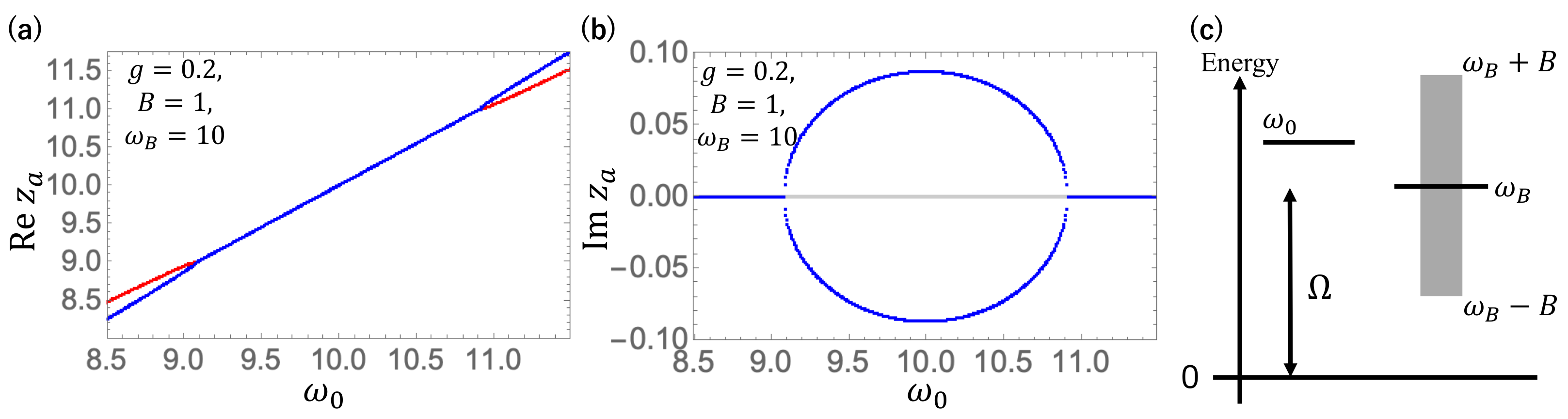
Now, we apply the method presented in the previous Sections to this specific case. In Figure 1, we show the complex eigenvalues of ${\mathit{L}}_{\mathrm{B}}$, $z_a$, obtained as a solution of Equation (27), for the molecular resonance eigenmode as a function of ${\omega }_0$, where we take ${\omega }_{\mathrm{B}}=10.0$, g = 0.2, $f_0$ = 1. The real and imaginary parts of $z_a$ are shown in Figure 1a and Figure 1b, respectively where the solutions on the first and second Riemann sheets are represented by the red and blue curves, respectively. The level scheme for these parameters is shown in Figure 1c. When the molecular oscillator is in resonance with the photonic band for ${\omega }_{\mathrm{B}}-B\lesssim {\omega }_0\lesssim {\omega }_{\mathrm{B}}+B$, one has complex eigenvalues of $z_a$, indicating that the excited molecular levels decay by emitting a photon into the photonic band. The branch points where the imaginary parts appear are known as the exceptional points.

Before showing the results of the photon emission spectrum, let us study the time evolution of the molecular excitation when the initial state is the unperturbed ground state. We derive the general expression of the molecular excitation with the use of the decomposition by the complex eigenmodes in Equation (A48). Substituting Equation (38) to Equation (A48), one has

$$\begin{array}{cc}\hfill & N_m(\mathrm{\Omega },t):=\langle 0|{\widehat{a}}^{†}(t)\widehat{a}(t)|0\rangle \hspace{1em}\hspace{1em}\hspace{1em}\hspace{1em}\hspace{1em}\hspace{1em}\hspace{1em}\hspace{1em}\hspace{1em}\hspace{1em}\hspace{1em}\hspace{1em}\hspace{1em}\hspace{1em}\hspace{1em}\hspace{1em}\hspace{1em}\hspace{1em}\hspace{1em}\hfill \end{array}$$

$$\begin{array}{cc}\hfill & =\frac{f_0^2}{4}{\left|{\int }_0^{t}d\tau (e^{i\mathrm{\Omega }\tau }+e^{-i\mathrm{\Omega }\tau })\left\{\langle a|{\phi }_a\rangle \langle {\tilde{\phi }}_a|a\rangle e^{-i{z}_a(t-\tau )}+\int dk\langle a|{\phi }_k\rangle \langle {\tilde{\phi }}_k|a\rangle e^{-i{\omega }_k(t-\tau )}\right\}\right|}^2\hfill \end{array}$$

(39)

$$\begin{array}{cc}\hfill & \simeq \frac{f_0^2}{4}{\left|{\mathcal{N}}_a\frac{e^{-i{z}_{a}t}-e^{-i\mathrm{\Omega }t}}{z_a-\mathrm{\Omega }}+\frac{1}{2\pi i}{\int }_{\mathrm{\Gamma }}d\omega \frac{1}{{\eta }_{\mathrm{\Gamma }}(\omega )}\frac{e^{-i\omega t}-e^{-i\mathrm{\Omega }t}}{\omega -\mathrm{\Omega }}\right|}^2,\hspace{1em}\hspace{1em}\hspace{1em}\hspace{1em}\hspace{1em}\hspace{1em}\hspace{1em}\hspace{1em}\hfill \end{array}$$

(40)

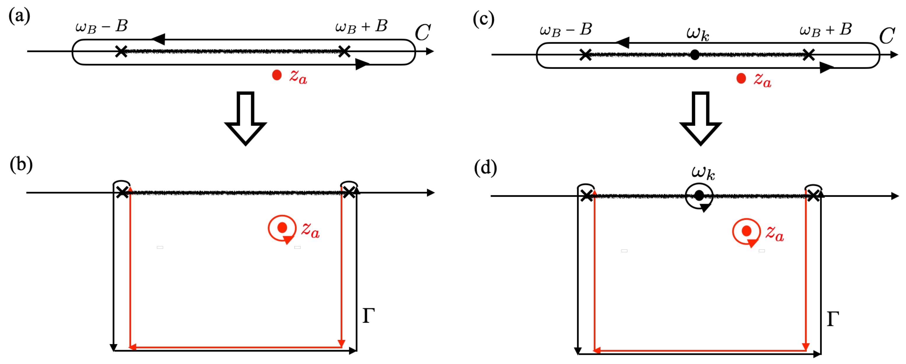
where, in Equation (40), we used the rotating wave approximation assuming the near-resonance situation, i.e., $\mathrm{\Omega }$≃${\omega }_0,{\omega }_B$. The detail of the derivation is explained in Appendix D. In Equation (40), the first term corresponds to the resonance mode. The second term corresponds to the so-called branch point effect [25,28,34], where $\mathrm{\Gamma }$ denotes the contour of the integral deformed to extract the branch point effect, as shown in Figure A1. The contour deformation to extract the branch point effect is given in Equation (A47) in Appendix D. The analytic continuation of ${\eta }_{\mathrm{\Gamma }}(z)$, defined in Equation (27), corresponds to the contour $\mathrm{\Gamma }$ in the Riemann sheets [34].

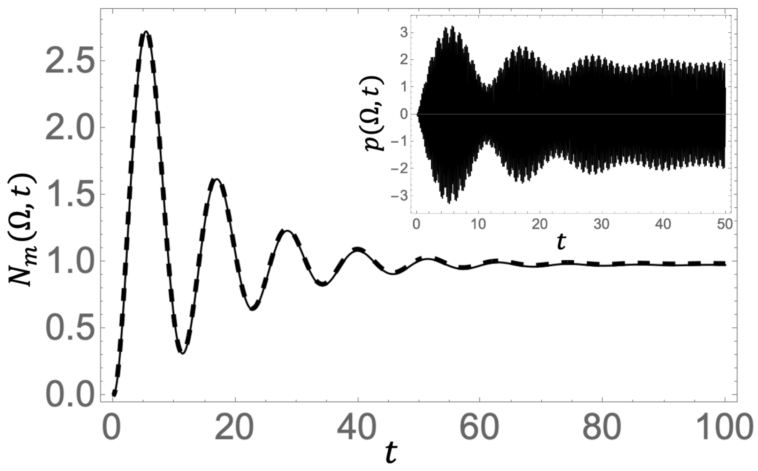
Figure 2 illustrates the time evolution of $N_m(\mathrm{\Omega },t)$ (solid curve) for parameters ${\omega }_0=10.5$, $\mathrm{\Omega }=10.0$, ${\omega }_B=10.0$, $g=0.2$, and $f_0=1$. In this case, the molecular oscillator is initially in the ground state, with the external field starting to act at $t=0$. One observes that $N_m(\mathrm{\Omega },t)$ oscillates in time with a Rabi frequency ($\mathrm{Re}\left[z_a\right]-\mathrm{\Omega }$) and eventually reaches a stationary value. We evaluate the long time limit of $N_m(\mathrm{\Omega },t)$. Since the time-dependent exponentials of the resonance pole and the branch point effect decay in the long time limit, we evaluate

$$\begin{array}{cc}\hfill \underset{t\to \infty }{lim}{N}_m(\mathrm{\Omega },t)& \simeq \frac{f_0^2}{4}{\left|{\mathcal{N}}_a\frac{1}{z_a-\mathrm{\Omega }}+\frac{1}{2\pi i}{\int }_{\mathrm{\Gamma }}d\omega \frac{1}{{\eta }_{\mathrm{\Gamma }}(\omega )}\frac{1}{\omega -\mathrm{\Omega }}\right|}^2\hspace{1em}\hspace{1em}\hspace{1em}\end{array}$$

(41)

$$\begin{array}{cc}\hfill & =\frac{f_0^2}{4}{\left|\frac{\langle a|{\phi }_a\rangle \langle {\tilde{\phi }}_a|a\rangle }{\mathrm{\Omega }-z_a}+\int dk\frac{\langle a|{\phi }_k\rangle \langle {\tilde{\phi }}_k|a\rangle }{\mathrm{\Omega }-{\omega }_k}\right|}^2\end{array}$$

(42)

$$\begin{array}{cc}\hfill & =\frac{f_0^2}{4}{\left|\langle a|\frac{1}{\mathrm{\Omega }-{\mathit{L}}_{\mathrm{B}}}|a\rangle \right|}^2=\frac{f_0^2}{4}\frac{1}{|{\eta }^{+}{(\mathrm{\Omega })|}^2}.\end{array}$$

(43)

We also show in the inset of Figure 2 the time evolution of the polarization of the molecule defined by

$$\begin{array}{c}\hfill p(\mathrm{\Omega },t):=\frac{1}{\sqrt{2{\omega }_0}}\langle 0|(\widehat{a}(t)+{\widehat{a}}^{†}(t))|0\rangle .\end{array}$$

(44)

This indicates that although the excitation population of the molecule remains constant in the steady state, the polarization oscillates rapidly with the external field frequency $\mathrm{\Omega }$. Our method effectively captures the time evolution of the entire system from the quantum vacuum to this nonequilibrium steady state under coherent driving. In particular, the contribution of the resonance mode is found to be dominant over the branch point effect, as long as the frequency of the molecular oscillator is far from the band edge.

We now shift our focus to the photon emission spectrum. The time–frequency-resolved photon emission spectrum is obtained as follows: Substituting Equation (38) to Equation (A50), one has

$$\begin{array}{cc}\hfill N_{\mathrm{ph}}({\omega }_k,\mathrm{\Omega },t)& :=\langle 0|{\widehat{b}}_k^{†}(t){\widehat{b}}_k(t)|0\rangle \rho ({\omega }_k)\hspace{1em}\hspace{1em}\hspace{1em}\hspace{1em}\hspace{1em}\hspace{1em}\hspace{1em}\hspace{1em}\hspace{1em}\hspace{1em}\hspace{1em}\hfill \end{array}$$

$$\begin{array}{cc}\hfill & =\frac{f_0^2\rho ({\omega }_k)}{4}{\left|{\int }_0^{t}d\tau (e^{i\mathrm{\Omega }\tau }+e^{-i\mathrm{\Omega }\tau })\frac{1}{2\pi i}{\oint }_{C}dw{e}^{-iw(t-\tau )}\langle b_k|\frac{1}{w-{\mathit{L}}_{\mathrm{B}}}|a\rangle \right|}^2\hfill \end{array}$$

(45)

$$\begin{array}{cc}\hfill & \simeq \frac{f_0^2\rho ({\omega }_k)}{4}{\left|{\int }_0^{t}d\tau e^{-i\mathrm{\Omega }\tau }\frac{1}{2\pi i}{\oint }_{C}dw{e}^{-iw(t-\tau )}\langle b_k|\frac{1}{w-{\mathit{L}}_{\mathrm{B}}}|a\rangle \right|}^2\hspace{1em}\hspace{1em}\hspace{1em}\hspace{1em}\hfill \end{array}$$

(46)

$$\begin{array}{cc}\hfill & =\frac{f_0^2{g}_k^2\rho ({\omega }_k)}{4}{\left|\frac{1}{2\pi }{\oint }_{C}dw\langle a|\frac{1}{w-{\mathit{L}}_{\mathrm{B}}}|a\rangle \frac{1}{w-{\omega }_k}\frac{e^{-i\mathrm{\Omega }t}-e^{-iwt}}{\mathrm{\Omega }-w}\right|}^2\hfill \\ \hfill & =\frac{f_0^2{g}_k^2\rho ({\omega }_k)}{4}\left|{\mathcal{N}}_a\frac{e^{-i{z}_{a}t}-e^{-i\mathrm{\Omega }t}}{z_a-\mathrm{\Omega }}\frac{1}{z_a-{\omega }_k}+\frac{e^{-i{\omega }_{k}t}-e^{-i\mathrm{\Omega }t}}{{\omega }_k-\mathrm{\Omega }}\frac{1}{{\eta }^{+}({\omega }_k)}\right.\hspace{1em}\hspace{1em}\hfill \end{array}$$

(47)

$$\begin{array}{cc}\hfill & {\left.+\frac{1}{2\pi i}{\int }_{\mathrm{\Gamma }}d\omega \frac{e^{-i\omega t}-e^{-i\mathrm{\Omega }t}}{\omega -\mathrm{\Omega }}\frac{1}{{\eta }_{\mathrm{\Gamma }}(\omega )}\frac{1}{\omega -{\omega }_k}\right|}^2,\hspace{1em}\hspace{1em}\hspace{1em}\hspace{1em}\hspace{1em}\hspace{1em}\hspace{1em}\hspace{1em}\hspace{1em}\hspace{1em}\hfill \end{array}$$

(48)

where $\rho (\omega )$ is the density of states of the photonic band given by

$$\begin{array}{c}\hfill \rho (\omega )=\frac{1}{\sqrt{B^2-{(\omega -{\omega }_B)}^2}}.\end{array}$$

(49)

In Equation (46), we use the rotating wave approximation. As shown in Appendix D, the contour of the integral C is deformed to extract the contributions of the resonance pole, the real pole, and the branch point effect, which are represented by the first, second, and third terms in Equation (48), respectively. One can see from Equation (A50) that the resonance pole contribution is attributed to the resonance eigenmode, while the real pole and the branch point contributions are attributed to the continuous eigenmode. This decomposition in terms of the complex eigenmodes gives a new perspective for understanding the photon emission spectrum.

Figure 3 shows the photon emission spectrum $N_{\mathrm{ph}}({\omega }_k,\mathrm{\Omega },t)$ at $t=100$, where the system is assumed to have reached the nonequilibrium steady state, as seen from Figure 2. One can see that there are two types of distinct spectral structures as a function of the driving field and the emitted photon energies, i.e., $\mathrm{\Omega }$ and ${\omega }_k$: one is a luminescence whose peak appears at ${\omega }_k\simeq {\omega }_0=10.5$ independent of $\mathrm{\Omega }$, and the other is a Rayleigh scattering whose peak is energetically correlated with $\mathrm{\Omega }$, i.e., appears at ${\omega }_k=\mathrm{\Omega }$. Our complex spectral analysis clarifies the different physical origins of the two peak structures. We give the explicit expression of the stationary photon emission spectrum in Equation (A54).

The luminescence is attributed to the resonance mode described by the first term of Equation (48), which has a Lorentzian spectral shape with peak position and width determined by $\mathrm{Re}\left[z_a\right]$ and $\mathrm{Im}\left[z_a\right]$, respectively. One can see that two variables, ${\omega }_k$ and $\mathrm{\Omega }$, are separated in the spectral function of the resonance mode component, so that the peak due to the resonance mode component appears just at ${\omega }_k=\mathrm{Re}{z}_a\simeq {\omega }_0$ independently of $\mathrm{\Omega }$. In other words, there is no energetic correlation between the driving field and luminescence. On the other hand, the coherent scattering is due to the real pole term of Equation (48), which makes the variables inseparable. The denominator of the first factor of the real pole term is mainly responsible for the Rayleigh scattering peak at ${\omega }_k=\mathrm{\Omega }$.

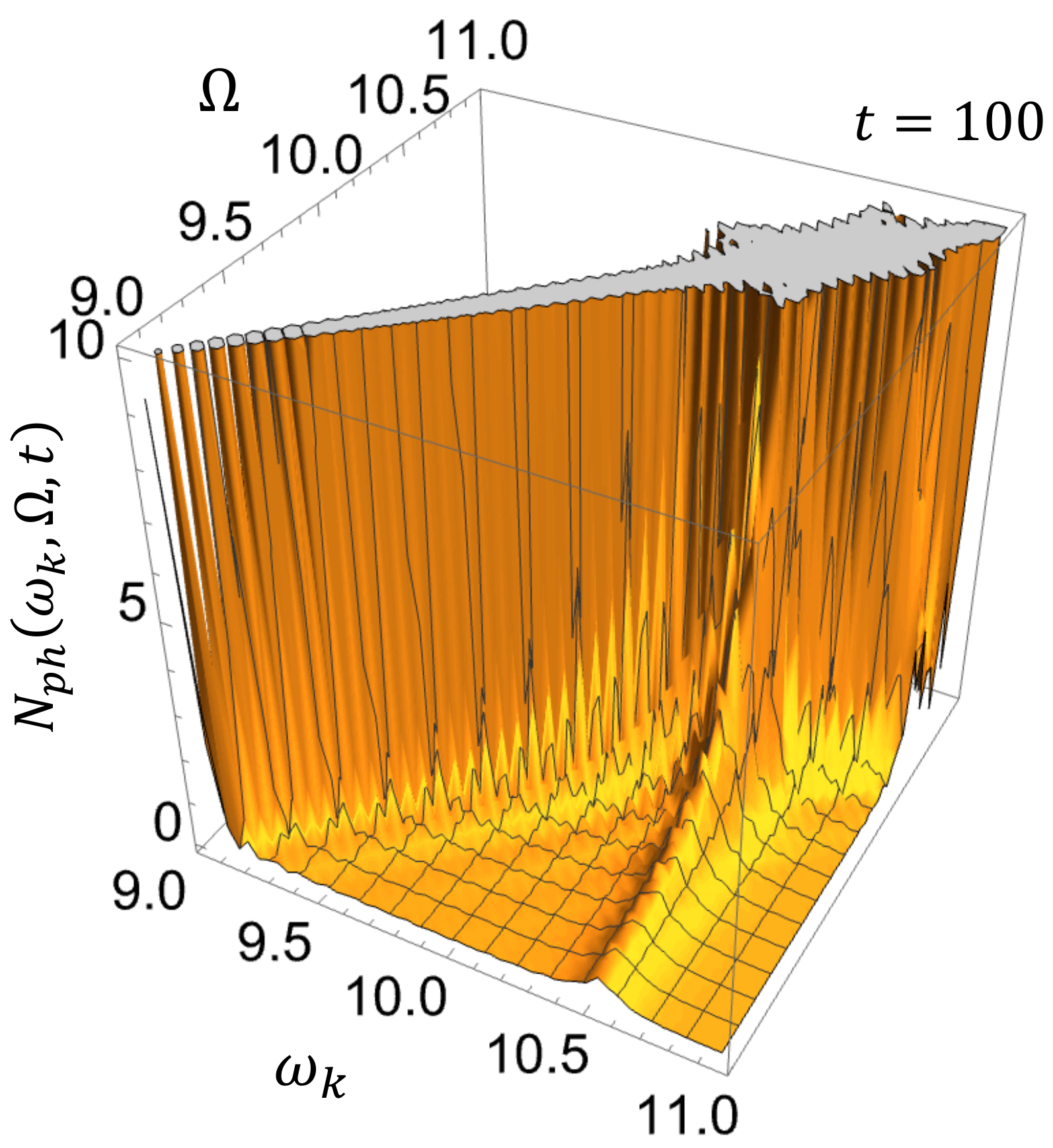
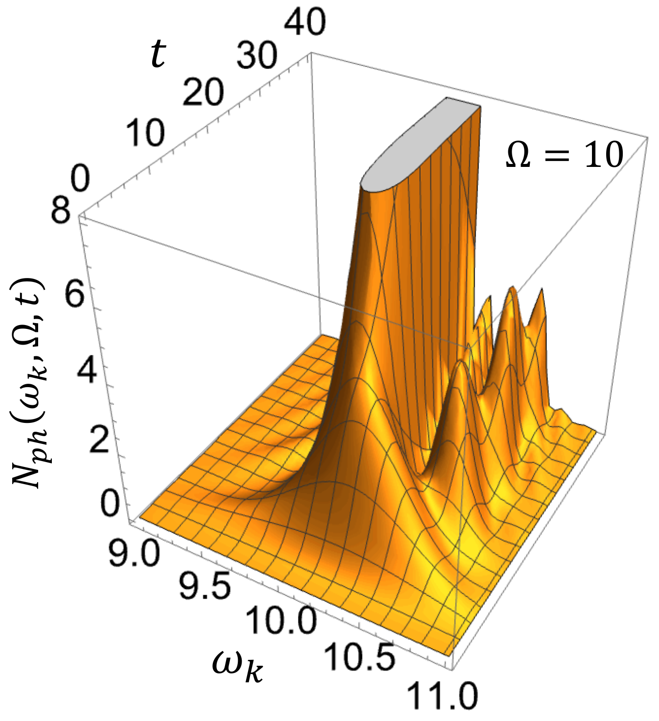
However, caution should be made before concluding that coherent scattering always occurs at ${\omega }_k=\mathrm{\Omega }$, while incoherent luminescence appears at ${\omega }_k\simeq {\omega }_0$. In Figure 4, we show the time–frequency-resolved photon emission spectrum for a driving frequency $\mathrm{\Omega }=10.0$ different from the molecular resonance frequency ${\omega }_0=10.5$, so that the Rayleigh peak and the luminescence can be seen separately, all other parameters being the same as in Figure 3. We observe that initially a broad spectrum is gradually built up with time, covering almost the entire photonic band $({\omega }_B-B=9.0<{\omega }_k<{\omega }_B+B=11.0)$. The broad spectrum is then separated into Rayleigh scattering at ${\omega }_k=\mathrm{\Omega }$ and luminescence at ${\omega }_k\simeq {\omega }_0$ during $t\simeq 10\sim 20$. Thereafter, the Rayleigh scattering peak grows proportional to $(f_0^2{g}_k^2\rho ({\omega }_k)/4|{\eta }^{+}({\omega }_k){|}^2)t^2$, while the luminescence shows an oscillatory behavior.

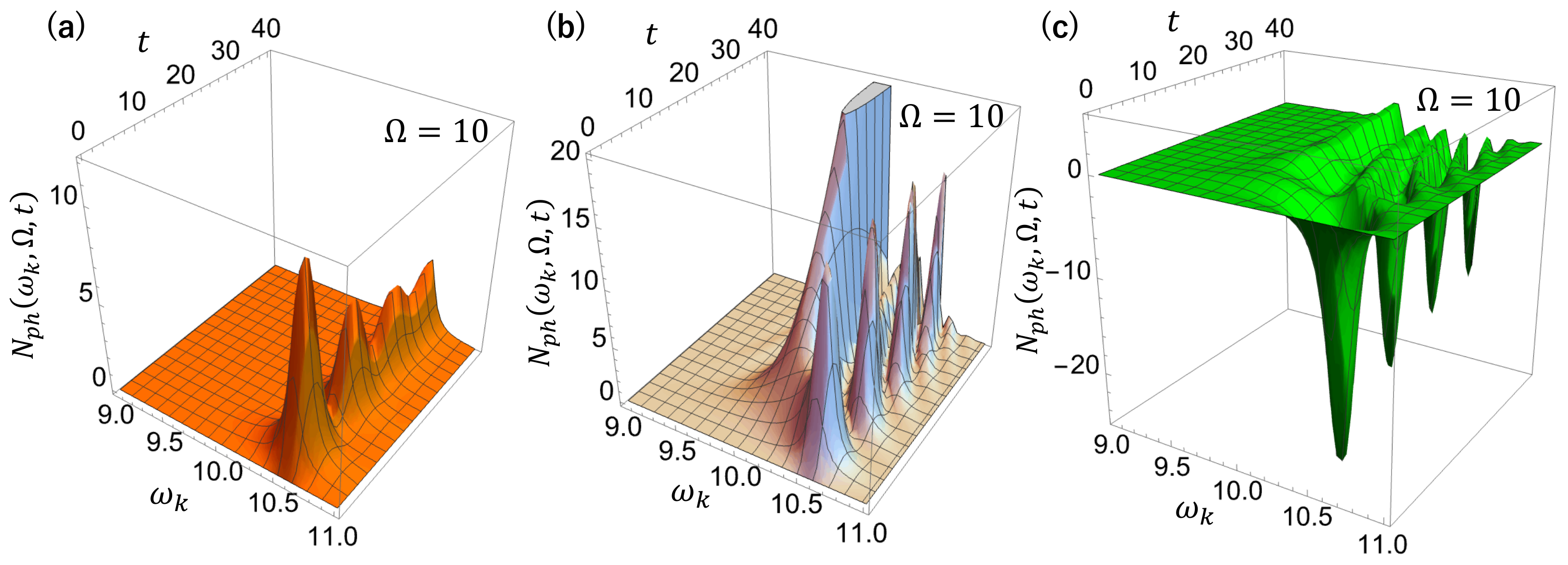
In order to clarify the origin of these spectral structures, we show in Figure 5 the time evolution of the spectral components of Figure 4, where the contributions of the resonance mode (Figure 5a), given by

$$\begin{array}{c}\hfill \frac{f_0^2{g}_k^2\rho ({\omega }_k)}{4}{\left|{\mathcal{N}}_a\frac{e^{-i{z}_{a}t}-e^{-i\mathrm{\Omega }t}}{z_a-\mathrm{\Omega }}\frac{1}{z_a-{\omega }_k}\right|}^2,\end{array}$$

(50)

the continuous mode (Figure 5b), given by

$$\begin{array}{c}\hfill \frac{f_0^2{g}_k^2\rho ({\omega }_k)}{4}{\left|\frac{e^{-i{\omega }_{k}t}-e^{-i\mathrm{\Omega }t}}{{\omega }_k-\mathrm{\Omega }}\frac{1}{{\eta }^{+}({\omega }_k)}\right|}^2,\end{array}$$

(51)

and the interference (Figure 5c), given by the cross-term between the two components, are shown separately. The resonance mode and continuous mode components, represented by the first and second terms in Equation (47), contribute to the spectrum, while the branch point effect represented by the third term in Equation (48), is negligible since ${\omega }_0$ is far from the photonic band edges.

As can be seen in Figure 5a, the resonance mode is responsible for the incoherent luminescence of an excited molecule, which peaks at ${\omega }_k=\mathrm{Re}{z}_a\simeq {\omega }_0$ with width $\mathrm{Im}{z}_a$ as a function of the emitted photon energy ${\omega }_k$. On the other hand, Rayleigh scattering at ${\omega }_k=\mathrm{\Omega }$ is solely due to the continuous mode component, as shown in Figure 5b. However, it is important to note that the continuous mode also plays a significant role in the spectral structure around ${\omega }_k\simeq {\omega }_0$. This specific contribution is derived from the resonance characteristic of ${\eta }^{+}({\omega }_k)$, as indicated in the second term of Equation (48).

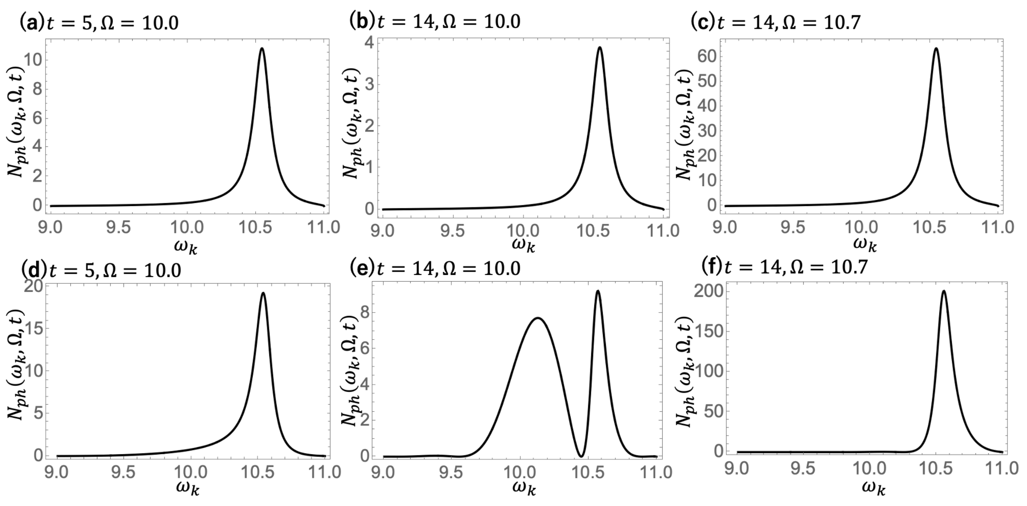
In order to reveal the characteristic difference between coherent scattering and incoherent luminescence, we show in Figure 6 the spectral functions of the resonance mode Equation (50) and continuous mode Equation (51) for different time t and driving field frequency $\mathrm{\Omega }$: Figure 6a–c for the resonance mode and Figure 6d–f for the continuous mode. It is seen that the spectral profile of the resonance mode component remains the same irrespective of variations in t and $\mathrm{\Omega }$, manifesting a Lorentzian spectral shape that peaks at ${\omega }_k=\mathrm{Re}{z}_a$ with a width of $\mathrm{Im}{z}_a$. The resonance mode component is therefore interpreted as incoherent luminescence from the excited molecule. In contrast, the spectral profile of the continuous mode with a peak around ${\omega }_k\simeq {\omega }_0$ varies with t and $\mathrm{\Omega }$. These results indicate that the photon emission associated with the continuous mode is coherent scattering, as the emitted photons are correlated with the incoming driving field.

This finding challenges the prevailing assumption that photon emission at the molecular excitation energy represents incoherent luminescence from an excited molecule. While the resonance component shown in Figure 5a converges to a constant in a manner consistent with the molecular excitation population shown in Figure 2, the spectral structure of the continuous mode component at the molecular resonance frequency shows an oscillation, as shown in Figure 5b. This oscillation effect contributes to the spectral structure at the molecular resonance. In addition, Figure 5c shows the presence of destructive interference between the resonance mode and the continuous mode components. This interference is responsible for the gradual build-up and broadness of the spectral structure observed during the early stages of the spectral evolution in Figure 4.

5. Concluding Remarks

We have presented a formulation for resonant photon emission from a molecular oscillator driven by a strong coherent laser field using complex spectral analysis of Liouvillian. In this paper, we considered the periodic shift of the equilibrium position of the oscillator induced by the strong driving field. In our theory, we treat the emitted radiation field quantum mechanically, including the radiation field as a part of the whole system as well as the molecular oscillator. Moreover, the theory extends the vector space to the rigged Hilbert space, which allows us to interpret the irreversible spontaneous emission process in the framework of quantum dynamics. We obtained the analytical solution of the Heisenberg equation in terms of the complex spectral analysis, with which the molecular excitation and the resonant photon emission spectrum were calculated. Thus, our theory succeeds in describing spontaneous emission, which requires both quantum vacuum fluctuation and irreversibility, in a unified way.

In contrast to the earlier studies [21,22,23], which solved a time-dependent Schrödinger equation for the matter prior to taking into account the interaction with the free radiation field, our theory first identifies the complex eigenmodes of the Liouvillian for the light–matter interacting system which are crucial for the spontaneous emission. Once we obtained the complex eigenmodes, the exact solution of the Heisenberg equation including the external field was immediately obtained without any approximation. Since the calculation is exact, our method continuously covers the weak coupling up to the strong coupling cases.

Our method clarifies the physical origin of the spectral structure by spectral decomposition in terms of eigenmodes. We confirm that the incoherent luminescence and coherent scattering are mainly due to the resonant mode and continuous components, respectively. However, our detailed spectral decomposition of the time–frequency-resolved photon emission shows that simplistic interpretations of the physical origin based on energetic correlations between the incident driving field and the emitted photon frequencies may be misleading. We found that the spectral structure around the molecular excitation is not only due to the resonance mode, but is also significantly influenced by the continuous mode, which differs from the time evolution of the molecular excitation. Furthermore, our study shows that destructive interference between these modes suppresses the spectral intensity in the early stages, leading to the formation of a broadband spectral structure.

In our study, we observed that branch point effects are insignificant in the results of Figure 2, Figure 3, Figure 4, Figure 5 and Figure 6. This is due to the fact that the spectral density evaluated by $\mathrm{Im}\mathrm{\Sigma }({\omega }_k)$ [40] approaches zero at the photonic band edges, ${\omega }_k={\omega }_{\mathrm{B}}\pm B$, a behavior illustrated in Figure 1b. In addition, the molecular frequency ${\omega }_0$ is significantly distant from these band edges. Nevertheless, the branch point effect becomes significant when ${\omega }_0$ is close to the band edges, especially when the spectral density has large values at these points. This can happen when the molecular dipole interacts with an infinite one-dimensional photonic band, where the spectral density diverges at the band edges by the Van Hove singularities [34]. Since the branch point effect has been identified as a key factor in the non-Markovian relaxation processes of excited states [41], the exaggeration of the non-Markovian effect due to the Van Hove singularities is worth further investigation [42,43].

In the present study, we showed the results for a long pulse case, where the envelope function is constant $f_0$. Our method can be applied to arbitrary envelope functions. Specifically, we found that the relative contribution of the resonance mode to that of the continuous modes is increased by shortening the pulse duration, making the incoherent luminescence prominent compared to the Rayleigh scattering. It is expected that the predictions of our theory can be tested experimentally using state-of-the-art pulse manipulation techniques.

Since the molecular oscillator in our study is a linear system, nonlinear phenomena such as high harmonic generation are not observed. Investigating the quantum properties of photon emission in high-harmonic generation through complex spectral analysis is an interesting topic for future research.