Casimir Energy in (2 + 1)-Dimensional Field Theories

Abstract

We explore the dependence of vacuum energy on the boundary conditions for massive scalar fields in (2 + 1)-dimensional spacetimes. We consider the simplest geometrical setup given by a two-dimensional space bounded by two homogeneous parallel wires in order to compare it with the non-perturbative behaviour of the Casimir energy for non-Abelian gauge theories in (2 + 1) dimensions. Our results show the existence of two types of boundary conditions which give rise to two different asymptotic exponential decay regimes of the Casimir energy at large distances. The two families are distinguished by the feature that the boundary conditions involve or not interrelations between the behaviour of the fields at the two boundaries. Non-perturbative numerical simulations and analytical arguments show such an exponential decay for Dirichlet boundary conditions of SU(2) gauge theories. The verification that this behaviour is modified for other types of boundary conditions requires further numerical work. Subdominant corrections in the low-temperature regime are very relevant for numerical simulations, and they are also analysed in this paper.

1. Introduction

The role of boundary effects in quantum field theory is fundamental for many quantum phenomena. One of the earliest applications was the Casimir effect [1]. A quantum field, when confined between two solid bodies, generates a dependence of the renormalized vacuum energy on the boundary conditions at the interfaces of the bodies. This dependence of the vacuum energy generates a force between them which depends on the nature of the boundary conditions of the quantum fields. Although this effect is very tiny, it has been experimentally measured in various setups [2,3,4,5,6,7].

A remarkable effort has been made in understanding and computing the Casimir effect for different models and setups. Some relevant results were obtained in Ref. [8], where the Casimir vacuum energy at zero temperature was computed for general boundary conditions and arbitrary dimensions for massless scalar fields using heat kernel methods. These results were later extended to finite temperatures in (3 + 1) dimensions [9].

Less known are the characteristics of the effect for interacting theories [10]. Quite recently, the behaviour of the Casimir energy has been investigated in (2 + 1)-dimensional Yang–Mills theories, where some reparametrization of gauge fields in terms of scalar fields allows for an analytic approach to the problem [11,12,13]. Numerical simulations with Dirichlet boundary conditions on gauge fields confirm the results of this analytic approach [14].

For $SU\left(2\right)$ gauge theories, the analytic approach is based on the description of gauge fields in terms of a massive scalar field, whose mass depends on the gauge coupling that in (2 + 1) dimensions is not dimensionless as in (3 + 1) dimensions. In that case, the Casimir energy of the strongly interacting gauge theories with Dirichlet boundary conditions coincides with the Casimir energy of a scalar field with a magnetic mass $m=g^2/\pi$, where g is the gauge coupling constant.

Some numerical simulations are in progress with different boundary conditions on gauge fields [15] to test if the relation between Casimir energy of massive fields and Yang–Mills theory is robust under the change in boundary conditions. Making comparisons with what happens for scalar fields requires knowing the behaviour of the Casimir energy of the massive scalars for different families of boundary conditions.

In this paper, we study the vacuum energy for massive scalar fields with general boundary conditions in a two-dimensional setup bounded by two homogeneous parallel wires by using a regularization scheme similar to the one used in Refs. [16,17] for massless theories. To compare our results with the lattice gauge theories’ results, it is necessary to work at a finite temperature; thus, it is important to understand how the thermal fluctuations affect the Casimir energy at low temperatures in both (2 + 1)-dimensional $SU\left(2\right)$ gauge theories and massive scalar field theories in order to have some analytical background reference to compare results to.

Independent of these motivations, some interest has been raised recently on the applications of the thermal Casimir effect in nano-electronic devices [18,19] or the appearance of negative self-entropy related to this effect [20,21,22], which has boosted interest in new aspects of these thermal effects.

2. Effective Action of a Massive Scalar Field in (2 + 1) Dimensions

We consider a free scalar massive field in (2 + 1) dimensions confined between two homogeneous infinite wires separated by a distance L. Depending on the structure of the wires, the quantum fields have to satisfy some conditions on the boundary wires. Moreover, finite temperature $T\ne 0$ effects can be described in the Euclidean formalism by compactification of the Euclidean time direction into a circle of radius $\beta /\left(2\pi \right)=1/\left(2\pi T\right)$. In this case, the partition function can be written as the following determinant:

$$Z\left(\beta \right)=\det {\left(-{\partial }_0^2-{𝝯}^2+m^2\right)}^{-1/2},$$

(1)

where m is the mass of the fields, ${𝝯}^2$ is the spatial Laplacian and ${\partial }_0$ is the Euclidean time derivative. As already mentioned, the boundary conditions are periodic in time $\psi (t+\beta ,\mathbf{x})=\psi (t,\mathbf{x})$, and because of the homogeneity of the boundary wires, the spatial boundary conditions can be given in terms of 2 × 2 unitary matrices $U\in$ U(2) [23]

$$\phi -i\delta \dot{\phi }=U(\phi +i\delta \dot{\phi }),$$

(2)

where $\delta$ is an arbitrary scale parameter and

$$\phi =\left(\begin{array}{c}\phi (L/2)\\ \phi (-L/2)\end{array}\right),\dot{\phi }=\left(\begin{array}{c}\dot{\phi }(L/2)\\ \dot{\phi }(-L/2)\end{array}\right),$$

(3)

are the boundary values $\phi (\pm L/2)=\psi (t,x_1,\pm L/2)$ of the fields $\psi$ and their outward normal derivatives $\dot{\phi }(\pm L/2)=\pm {\partial }_2\psi (t,x_1,\pm L/2)$ on the wires. From now on, we will assume that $\delta =1$ for simplicity.

In the standard parametrization of U(2) matrices

$$\begin{array}{ccc}\hfill U(\alpha ,\gamma ,\mathbf{n})& =& {\mathrm{e}}^{i\alpha }\left(\mathbb{I}cos\gamma +i\mathbf{n}·\mathit{\sigma }sin\gamma \right);\alpha \in [0,2\pi ],\gamma \in [-\pi /2,\pi /2],\hfill \end{array}$$

(4)

in terms of a unit vector $\mathbf{n}\in S^2$ and Pauli matrices $\mathit{\sigma }=({\sigma }_1,{\sigma }_2,{\sigma }_3)$, the space of boundary conditions that preserve the non-negativity of the spectrum of the operator $-{𝝯}^2$ is restricted by the inequalities $0\le \alpha \pm \gamma \le \pi$ [8]. Moreover, since the scalar field is real, the second component of the unit vector n has to vanish, i.e., $n_2=0$.

The determinant of the second-order differential operator $-{\partial }_0^2-{𝝯}^2+m^2$ in Equation (1) is ultraviolet (UV) divergent but can be regularized by means of the zeta regularization method [24,25]. The effective action is defined by the logarithm of the partition function, which can be expressed as

$$S_{\mathrm{eff}}=-\log Z=-\frac{1}{2}\frac{d}{ds}\zeta \left(s\right){|}_{s=0},$$

(5)

and in terms of the zeta function as

$$\zeta (L,m,\beta ;s)={\mu }^{2s}{\left(-{\partial }_0^2-{𝝯}^2+m^2\right)}^{-s}$$

(6)

where we have introduced the scale parameter $\mu$, which encodes the standard ambiguity of zeta function renormalization techniques (see, e.g., [26,27] for a detailed discussion and comparison with other renormalization methods), to make the zeta function dimensionless. This ambiguity will be fixed by the renormalization scheme prescription. Actually, the scale parameter $\mu$ can be seen as an explicit implementation of the renormalization group.

In our case of a massive scalar field confined between two infinite wires, the eigenvalues of operator $-{\partial }_0^2-{𝝯}^2$ are given by the sum of the square of the temporal modes $2\pi l/\beta$ associated with the Matsubara frequencies, the continuous spatial modes k, and the discrete spatial modes $k_i$ that depend on the boundary conditions imposed by the boundary wires

$$\lambda ={\left(\frac{2\pi l}{\beta }\right)}^2+k^2+k_i^2+m^{2}l\in \mathbb{Z},i\in \mathbb{N}.$$

(7)

Thus, the zeta function in this case reads as follows:

$$\zeta (L,m,\beta ;s)={\mu }^{2s}\frac{A}{2\pi }\sum _{l,i}{\int }_{-\infty }^{\infty }dk{\left({\left(\frac{2\pi l}{\beta }\right)}^2+k^2+k_i^2+m^2\right)}^{-s},$$

(8)

where A is the length of the wires. Now, we can integrate the continuous spatial modes using the analytic extension of the zeta function

$$\zeta (L,m,\beta ;s)={\mu }^{2s}\frac{A\mathsf{\Gamma }(s-1/2)}{2\sqrt{\pi }\mathsf{\Gamma }\left(s\right)}\sum _{l,i}{\left({\left(\frac{2\pi l}{\beta }\right)}^2+k_i^2+m^2\right)}^{-s+1/2}.$$

(9)

It was shown in Ref. [8] that for homogeneous boundary conditions along the wires, the discrete spatial modes are given by the zeros of the spectral function

$$h_U^L\left(k\right)=sin\left(kL\right)\left((k^2-1)cos\gamma +(k^2+1)cos\alpha \right)-2ksin\alpha cos\left(kL\right)-2k{n}_{1}sin\gamma ,$$

(10)

in the following way

$$\zeta (L,m,\beta ;s)={\mu }^{2s}\frac{A\mathsf{\Gamma }(s-1/2)}{4{\pi }^{3/2}i\mathsf{\Gamma }\left(s\right)}\sum _{l=-\infty }^{\infty }\oint dk{\left({\left(\frac{2\pi l}{\beta }\right)}^2+k^2+m^2\right)}^{-s+1/2}\frac{d}{dk}\log h_U^L\left(k\right),$$

(11)

where the integral is defined along the contour of a thin strip enclosing the positive real axis, where all the zeros of the spectral function $h_U\left(k\right)$ are located.

All ultraviolet divergences arise in the zero temperature limit of the vacuum energy and the removal of such divergences requires a consistent prescription method (renormalization scheme) with a clear physical meaning. They appear in the leading terms of the zero-temperature expansion that has the following asymptotic behaviour in the large L limit [8,16]:

$$S_{\mathrm{eff}}^{l=0}=\beta E_0=C_0\left(m\right)A\beta L+C_1\left(m\right)A\beta +\frac{A\beta }{L}{C}_c(m,L)+\dots .$$

(12)

where $E_0$ is the vacuum energy, $C_0\left(m\right)$ the divergent bulk vacuum energy density, $C_1\left(m\right)$ the divergent energy density of the boundary wires, and $C_c(m,L)$ is the finite coefficient of the Casimir energy.

One renormalization prescription which allows us to eliminate all these divergences consists of the redefinition of the renormalized effective action as follows [16,17]:

$$S_{\mathrm{eff}}^{\mathrm{ren}}=-\frac{1}{2}\frac{d}{ds}{\zeta }_{\mathrm{ren}}(L,m,\beta ;s){|}_{s=0},$$

(13)

where

$${\zeta }_{\mathrm{ren}}(L,m,\beta ;s)=\underset{L_0\to \infty }{\lim }\left(\zeta (L,m,\beta ;s)+\zeta (2L_0+L,m,\beta ;s)-2\zeta (L_0+L,m,\beta ;s)\right),$$

(14)

in terms of an auxiliary length $L_0$. Notice that the physical condition which fixes this renormalization scheme is the complete removal of the spurious contributions to the bulk and the boundary vacuum energies, leaving only Casimir energy terms and nonlinear $\beta$-temperature-dependent contributions to the effective action. These are precisely the physical requirements that fix the renormalization scheme’s prescription.

The sum over Matsubara modes can be explicitly computed in the low-temperature regime.

3. Low-Temperature Regime

In the low-temperature limit $\beta m\gg 1$, we cannot express the result as an infinite series of $1/\beta$. This means that we have to first deal with the Matsubara modes and later with the boundary modes. We start by rewriting (9) as follows:

$$\zeta (L,m,\beta ;s)={\left(\frac{\mu \beta }{2\pi }\right)}^{2s}\frac{A\sqrt{\pi }\mathsf{\Gamma }(s-1/2)}{\beta \mathsf{\Gamma }\left(s\right)}\sum _i\sum _{l=-\infty }^{\infty }{\left(l^2+{\left(\frac{k_i\beta }{2\pi }\right)}^2+{\left(\frac{m\beta }{2\pi }\right)}^2\right)}^{-s+1/2}.$$

(15)

Now, we use the Mellin transform

$$\zeta (L,m,\beta ;s)={\left(\frac{\mu \beta }{2\pi }\right)}^{2s}\frac{A\sqrt{\pi }}{\beta \mathsf{\Gamma }\left(s\right)}\sum _i\sum _{l=-\infty }^{\infty }{\int }_0^{\infty }dt{t}^{s-3/2}{e}^{-\left(l^2+{\left(\frac{k_i\beta }{2\pi }\right)}^2+{\left(\frac{m\beta }{2\pi }\right)}^2\right)t}$$

(16)

and apply the Poisson formula for the sum over l modes

$$\zeta (L,m,\beta ;s)={\left(\frac{\mu \beta }{2\pi }\right)}^{2s}\frac{A\pi }{\beta \mathsf{\Gamma }\left(s\right)}\sum _i\sum _{l=-\infty }^{\infty }{\int }_0^{\infty }dt{t}^{s-2}{e}^{-\left({\left(\frac{k_i\beta }{2\pi }\right)}^2+{\left(\frac{m\beta }{2\pi }\right)}^2\right)t-\frac{{\left(\pi l\right)}^2}{t}}.$$

(17)

We can compute the integral

$$\begin{array}{cc}\hfill \zeta (L,m,\beta ;s)& ={\left(\frac{\mu \beta }{2\pi }\right)}^{2s}\frac{A\pi }{\beta \mathsf{\Gamma }\left(s\right)}\left(\mathsf{\Gamma }\left(s-1\right)\sum _i{\left({\left(\frac{k_i\beta }{2\pi }\right)}^2+{\left(\frac{m\beta }{2\pi }\right)}^2\right)}^{1-s}\right.\hfill \\ \hfill & \left.+4\sum _i\sum _{l=1}^{\infty }{\left(\pi l\right)}^{-1+s}{\left({\left(\frac{k_i\beta }{2\pi }\right)}^2+{\left(\frac{m\beta }{2\pi }\right)}^2\right)}^{1/2-s/2}{K}_{1-s}\left(\beta l\sqrt{k_i^2+m^2}\right)\right),\hfill \end{array}$$

(18)

where we have obtained a term ($l=0$) that has a linear dependence on $\beta$, and the rest of the terms can be expressed in terms of the modified Bessel function of the second type $K_{\nu }$. Let us focus on the first term, which is the zero-temperature one, by replacing the sum of boundary modes with an integral modulated by the spectral function (10). We have

$${\zeta }^{l=0}(L,m,\beta ;s)={\mu }^{2s}\frac{A\beta \mathsf{\Gamma }\left(s-1\right)}{8{\pi }^{2}i\mathsf{\Gamma }\left(s\right)}\oint dk{\left(k^2+m^2\right)}^{1-s}\frac{d}{dk}\log h_U^L\left(k\right).$$

(19)

Thus, the zero-temperature term of the renormalized zeta (14) is

$${\zeta }_{\mathrm{ren}}^{l=0}(L,m,\beta ;s)={\mu }^{2s}\frac{A\beta \mathsf{\Gamma }\left(s-1\right)}{8{\pi }^{2}i\mathsf{\Gamma }\left(s\right)}\underset{L_0\to \infty }{\lim }\oint dk{\left(k^2+m^2\right)}^{1-s}\frac{d}{dk}\log \frac{h_U^L\left(k\right)h_U^{2L_0+L}\left(k\right)}{{\left(h_U^{L_0+L}\left(k\right)\right)}^2}.$$

(20)

As it was explained previously, this combination cancels the UV divergences on the integral; thus, the only divergent terms left are the ratio of two Gamma functions whose asymptotic behaviour in the small s expansion is

$$\frac{\mathsf{\Gamma }(s-1)}{\mathsf{\Gamma }\left(s\right)}=-1-s+\mathcal{O}\left(s^2\right)$$

(21)

which allows us to calculate the derivative

$$\frac{d}{ds}{\left.\left(-\left(1+s\right){\left(k^2+m^2\right)}^{1-s}{\mu }^{2s}\right)\right|}_{s=0}=(k^2+m^2)\left(\log \left(k^2+m^2\right)-2\log \mu -1\right).$$

(22)

Thus, we have

$$\begin{array}{cc}\hfill {\left({\zeta }_{\mathrm{ren}}^{l=0}\right)}^{\prime }(L,m,\beta ;0)=\frac{A\beta }{8{\pi }^{2}i}\underset{L_0\to \infty }{\lim }\oint dk& \left(k^2+m^2\right)\left(\log \left(k^2+m^2\right)-2\log \mu -1\right)\hfill \\ \hfill & \times \left(\frac{d}{dk}\log \frac{h_U^L\left(k\right)h_U^{2L_0+L}\left(k\right)}{{\left(h_U^{L_0+L}\left(k\right)\right)}^2}\right).\hfill \end{array}$$

(23)

Since the integrand is holomorphic, we can extend the integration contour to an infinite semicircle limited by the imaginary axis on its left. Also, because the integration over the semicircle is zero, we can reduce the integral to the imaginary axis

$$\begin{array}{cc}\hfill {\left({\zeta }_{\mathrm{ren}}^{l=0}\right)}^{\prime }(L,m,\beta ;0)=\frac{A\beta }{8{\pi }^{2}i}\underset{L_0\to \infty }{\lim }{\int }_{-\infty }^{\infty }dk\left(k^2-m^2\right)& \left(\log \left(m^2-k^2\right)-2\log \mu -1\right)\hfill \\ & \times \left(\frac{d}{dk}\log \frac{h_U^L\left(ik\right)h_U^{2L_0+L}\left(ik\right)}{{\left(h_U^{L_0+L}\left(ik\right)\right)}^2}\right).\hfill \end{array}$$

(24)

Taking into account that the integrand is parity odd, the integral would vanish if it were not for the contribution of the branching point $k=m$ of the logarithm $\log (m^2-k^2)$, which gives a factor $2\pi i$ for the interval $(m,\infty )$, which is absent in the interval $(-\infty ,-m)$. Thus, the expression reduces to

$${\left({\zeta }_{\mathrm{ren}}^{l=0}\right)}^{\prime }(L,m,\beta ;0)=\frac{A\beta }{4\pi }\underset{L_0\to \infty }{\lim }{\int }_m^{\infty }dk\left(k^2-m^2\right)\frac{d}{dk}\log \frac{h_U^L\left(ik\right)h_U^{2L_0+L}\left(ik\right)}{{\left(h_U^{L_0+L}\left(ik\right)\right)}^2}.$$

(25)

Since the integral domain begins at m, we can take the limit $L_0\to \infty$ on the spectral functions by noticing that

$$\underset{L_{*}\to \infty }{\lim }{h}_U^{L_{*}}\left(ik\right)=\underset{L_{*}\to \infty }{\lim }{e}^{k\left(L_{*}\right)}\left((k^2+1)cos\gamma +(k^2-1)cos\alpha +2ksin\alpha \right).$$

(26)

If we define the result in terms of the limit for the spectral function

$$h_U^{\infty }\left(ik\right)\equiv \left((k^2+1)cos\gamma +(k^2-1)cos\alpha +2ksin\alpha \right),$$

(27)

we obtain a simplified formula:

$${\left({\zeta }_{\mathrm{ren}}^{l=0}\right)}^{\prime }(L,m,\beta ;0)=-\frac{A\beta }{4\pi }{\int }_m^{\infty }dk\left(k^2-m^2\right)\left(L-\frac{d}{dk}\log \frac{h_U^L\left(ik\right)}{h_U^{\infty }\left(ik\right)}\right).$$

(28)

Temperature-Dependent Terms

Let us now compute the terms with $l\ne 0$ of the zeta function

$$\begin{array}{cc}\hfill {\zeta }^{l\ne 0}(L,m,\beta ;s)={\left(\frac{\mu \beta }{2\pi }\right)}^{2s}\frac{4A\pi }{\beta \mathsf{\Gamma }\left(s\right)}\sum _{i,l=1}{\left(\pi l\right)}^{-1+s}& {\left({\left(\frac{k_i\beta }{2\pi }\right)}^2+{\left(\frac{m\beta }{2\pi }\right)}^2\right)}^{1/2-s/2}\hfill \\ \hfill & \times \left(K_{1-s}\left(\beta l\sqrt{k_i^2+m^2}\right)\right).\hfill \end{array}$$

(29)

Since the Bessel special function $K_1$ decreases exponentially as the argument grows, both sums are finite; thus, the only divergent contribution is the Gamma function, which after derivation gives

$${\left({\zeta }^{l\ne 0}\right)}^{\prime }(L,m,\beta ;0)=\frac{2A}{\pi }\sum _i\sum _{l=1}^{\infty }\frac{\sqrt{k_i^2+m^2}}{l}{K}_1\left(\beta l\sqrt{k_i^2+m^2}\right)$$

(30)

and we can we rewrite the sum of the discrete eigenvalues by means of the spectral Formula (10)

$${\left({\zeta }^{l\ne 0}\right)}^{\prime }(L,m,\beta ;0)=\frac{A}{{\pi }^{2}i}\sum _{l=1}^{\infty }\oint dk\frac{\sqrt{k^2+m^2}}{l}{K}_1\left(\beta l\sqrt{k^2+m^2}\right)\frac{d}{dk}\log \left(h_U^L\left(k\right)\right).$$

(31)

Thus, the temperature-dependent terms of the renormalized zeta function (14) have the following form:

$${\left({\zeta }_{\mathrm{ren}}^{l\ne 0}\right)}^{\prime }(L,m,\beta ;0)=\frac{A}{{\pi }^{2}i}\underset{L_0\to \infty }{\lim }\sum _{l=1}^{\infty }\oint dk\frac{\sqrt{k^2+m^2}}{l}{K}_1\left(\beta l\sqrt{k^2+m^2}\right)\frac{d}{dk}\log \frac{h_U^L\left(k\right)h_U^{2L_0+L}\left(k\right)}{{\left(h_U^{L_0+L}\left(k\right)\right)}^2}.$$

In a similar manner as was carried out for the $l=0$ term, since the integrand is also holomorphic we can extend the contour to an infinite semi-circle limited by the imaginary axis. Because the integral is zero on the semi-circle, we can reduce the integral to just the imaginary axis

$$\begin{array}{cc}\hfill {\left({\zeta }_{\mathrm{ren}}^{l\ne 0}\right)}^{\prime }(L,m,\beta ;0)=-\frac{A}{{\pi }^{2}i}\underset{L_0\to \infty }{\lim }\sum _{l=1}^{\infty }{\int }_{-\infty }^{\infty }& dk\frac{\sqrt{-k^2+m^2}}{l}{K}_1\left(\beta l\sqrt{-k^2+m^2}\right)\hfill \\ \hfill & \times \left(\frac{d}{dk}\log \frac{h_U^L\left(ik\right)h_U^{2L_0+L}\left(ik\right)}{{\left(h_U^{L_0+L}\left(ik\right)\right)}^2}\right).\hfill \end{array}$$

(32)

Because the integrand is odd, the contribution of $(-m,m)$ is zero, whereas the branching point of $\sqrt{m^2-k^2}$ introduces a change of sign on the integrand on $(-\infty ,-m)$ and also in the argument of the Bessel function. Given that $K_1\left(\overline{z}\right)=\overline{K_1\left(z\right)}$, the real part of the integrals between $(-\infty ,-m)$ and $(m,\infty )$ is twice one of the integrals, whereas the imaginary part cancels out. In summary, the integral can be reduced to

$$\begin{array}{cc}\hfill {\left({\zeta }_{\mathrm{ren}}^{l\ne 0}\right)}^{\prime }(L,m,\beta ;0)=-\frac{2A}{{\pi }^2}\underset{L_0\to \infty }{\lim }\sum _{l=1}^{\infty }{\int }_m^{\infty }& dk\frac{\sqrt{k^2-m^2}}{l}\Re \left(K_1\left(i\beta l\sqrt{k^2-m^2}\right)\right)\hfill \\ \hfill & \times \left(\frac{d}{dk}\log \frac{h_U^L\left(ik\right)h_U^{2L_0+L}\left(ik\right)}{{\left(h_U^{L_0+L}\left(ik\right)\right)}^2}\right).\hfill \end{array}$$

(33)

We can take the limit $L_0\to \infty$ using Equation (26) as we did for the $l=0$ term, and the integral is simplified to

$${\left({\zeta }_{\mathrm{ren}}^{l\ne 0}\right)}^{\prime }(L,m,\beta ;0)=\frac{2A}{{\pi }^2}\sum _{l=1}^{\infty }{\int }_m^{\infty }dk\frac{\sqrt{k^2-m^2}}{l}\Re \left(K_1\left(i\beta l\sqrt{k^2-m^2}\right)\right)\left(L-\frac{d}{dk}\log \frac{h_U^L\left(ik\right)}{h_U^{\infty }\left(ik\right)}\right).$$

4. Casimir Energy

The Casimir energy can be derived from the terms we have just computed in the previous sections. We can easily compute the free energy with the effective action simply using the expression $F=S_{\mathrm{eff}}/\beta$. This free energy has two different contributions [22], the non-temperature-dependent part ($l=0$) which corresponds to the Casimir energy of the system

$$F_U^{l=0}(L,m,\beta )=E_U^c(L,m)=\frac{A}{8\pi }{\int }_m^{\infty }dk\left(k^2-m^2\right)\left(L-\frac{d}{dk}\log \frac{h_U^L\left(ik\right)}{h_U^{\infty }\left(ik\right)}\right),$$

(34)

and the temperature-dependent part

$$F_U^{l\ne 0}(L,m,\beta )=-\frac{A}{\beta {\pi }^2}\sum _{l=1}^{\infty }{\int }_m^{\infty }dk\frac{\sqrt{k^2-m^2}}{l}\Re \left(K_1\left(i\beta l\sqrt{k^2-m^2}\right)\right)\left(L-\frac{d}{dk}\log \frac{h_U^L\left(ik\right)}{h_U^{\infty }\left(ik\right)}\right).$$

Both terms of the free energy decrease to zero as the distance between the wires L grows to infinite, which is the expected behaviour. The temperature-dependent term also vanishes $F_U^{l\ne 0}\to 0$ when the temperature does ($\beta \to \infty$).

Asymptotic Behaviour

Let us now analyse the behaviour of the Casimir energy when $mL\to \infty$. First, we rewrite the hyperbolic functions of the spectral function as

$$h_U^L\left(ik\right)=e^{kL}\left((k^2+1)cos\gamma +(k^2-1)sin\alpha +2ksin\alpha \right)\left(1+n_{1}sin\left(\gamma \right)\mathcal{A}{e}^{-kL}+\mathcal{B}{e}^{-2kL}\right),$$

where $\mathcal{A}$ and $\mathcal{B}$ are

$$\begin{array}{cc}\hfill & \mathcal{A}(k,\alpha ,\gamma )=\frac{4k}{(k^2+1)cos\gamma +(k^2-1)sin\alpha +2ksin\alpha },\hfill \end{array}$$

(35)

$$\begin{array}{cc}\hfill & \mathcal{B}(k,\alpha ,\gamma )=\frac{-(k^2+1)cos\gamma -(k^2-1)sin\alpha +2ksin\alpha }{(k^2+1)cos\gamma +(k^2-1)sin\alpha +2ksin\alpha }.\hfill \end{array}$$

(36)

We can use this expression to approximate the logarithm of the quotient of spectral functions as

$$\log \frac{h_U^L\left(ik\right)}{h_U^{\infty }\left(ik\right)}=kL+n_{1}sin\gamma \mathcal{A}{e}^{-kL}+(\mathcal{B}-\frac{{\mathcal{A}}^{\prime }}{2})e^{-2kL}+O\left(e^{-3kL}\right),$$

(37)

where ${\mathcal{A}}^{\prime }={(n_{1}sin\left(\gamma \right)\mathcal{A})}^2$, and we expand the logarithm in powers of $e^{-kL}$. Now, we introduce this expression on the integral of the Casimir energy formula

$$\begin{array}{cc}\hfill E_U^c& =-\frac{A}{8\pi }{\int }_m^{\infty }dk(k^2-m^2)\frac{d}{dk}\left(n_{1}sin\gamma \mathcal{A}{e}^{-kL}+(\mathcal{B}-\frac{{\mathcal{A}}^{\prime }}{2})e^{-2kL}+O\left(e^{-3kL}\right)\right)\hfill \\ \hfill & =\frac{A}{4\pi }{\int }_m^{\infty }dkk\left(n_{1}sin\gamma \mathcal{A}{e}^{-kL}+(\mathcal{B}-\frac{{\mathcal{A}}^{\prime }}{2})e^{-2kL}+O\left(e^{-3kL}\right)\right).\hfill \end{array}$$

(38)

We can expand this integral as a power series of $1/L$ for each exponential order by integrating by parts as follows:

$${\int }_m^{\infty }dkg(\alpha ,\gamma ,n_1,k)e^{-jkL}=-{\left.\frac{g(\alpha ,\gamma ,n_1,k)}{jL}{e}^{-jkL}\right|}_m^{\infty }+{\int }_m^{\infty }dk\frac{g{(\alpha ,\gamma ,n_1,k)}^{\prime }}{jL}{e}^{-jkL},$$

(39)

and iterate this process since all derivatives of $g(\alpha ,\gamma ,n_1,k)$ are regular in $[m,\infty ]$. Thus, the Casimir energy is given by

$$E_U^c=\sum _{j=1}^{\infty }\sum _{\nu =1}^{\infty }\frac{c_{j,\nu }(\alpha ,\gamma ,n_1,m)}{{\left(jL\right)}^{\nu }}{e}^{-jmL},$$

(40)

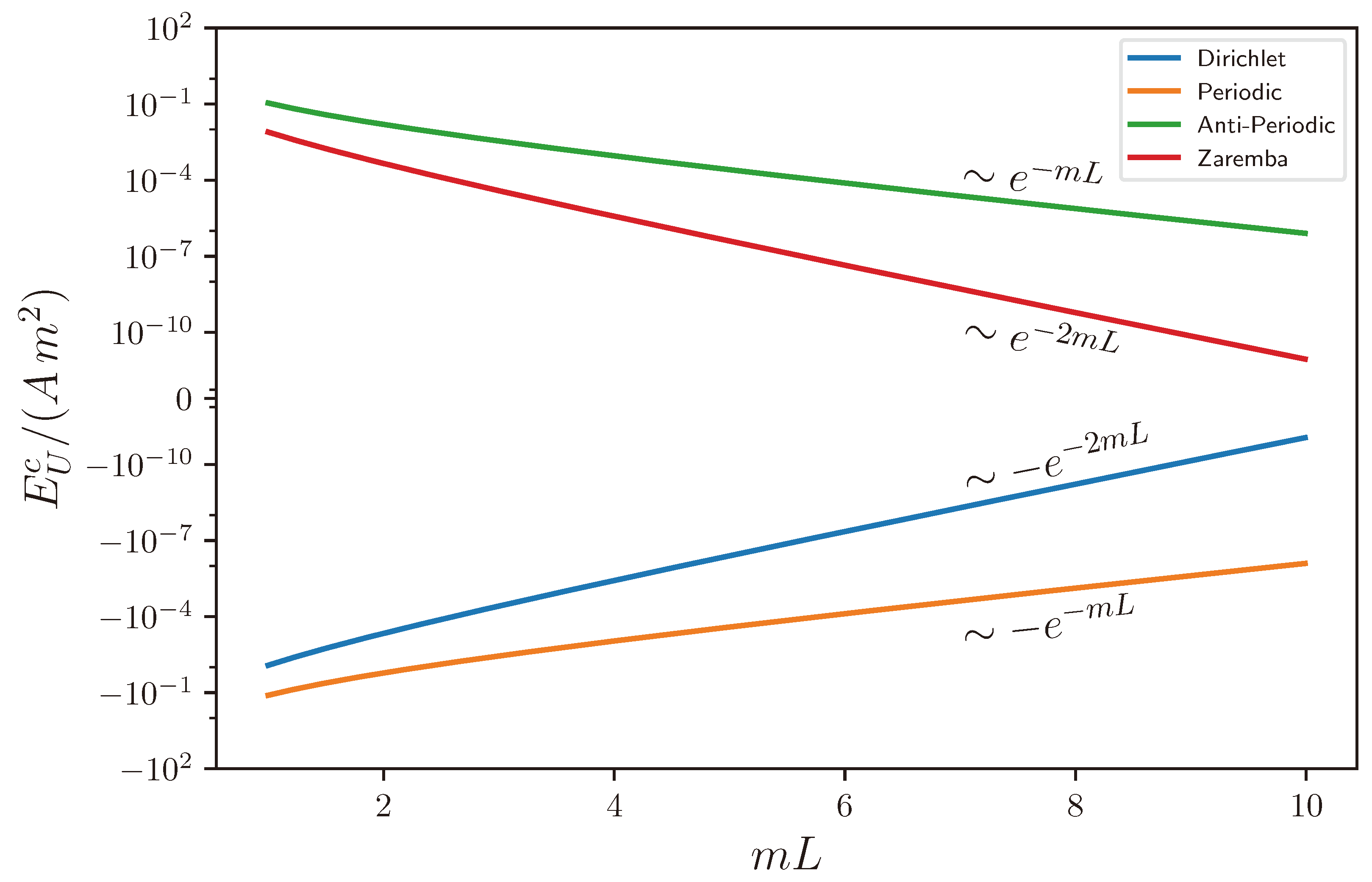
where the coefficients corresponding to the leading order in the exponential expansion are of the form

$$c_{1,\nu }=-\frac{n_{1}sin\gamma }{4\pi }{\left.\frac{d^{\nu }\left(k\mathcal{A}(\alpha ,\gamma ,k)\right)}{d{k}^{\nu }}\right|}_m^{\infty }.$$

(41)

This means that when $n_{1}sin\gamma =0$, all the terms that behave as $e^{-mL}$ vanish and the leading contribution will be of the order of $e^{-2mL}$. Thus, we have two different families of boundary conditions with different asymptotic behaviours

$$L{E}_U^c\sim \left\{\begin{array}{cc}{e}^{-mL}& \mathrm{if}\mathrm{tr}\left(U{\sigma }_1\right)\ne 0,\\ e^{-2mL}& \mathrm{if}\mathrm{tr}\left(U{\sigma }_1\right)=0,\end{array}\right.$$

(42)

depending on whether the matrix U that defines the boundary conditions depends or not on ${\sigma }_1$.

This is the most important result of this paper because it classifies the boundary conditions into two families. The difference between the two families is the rate of the exponential decay of the Casimir energy (42).

The physical characterization of the two families of boundary conditions with different exponential decays is the vanishing or not of $\mathrm{tr}\left(U{\sigma }_1\right)$. The non-vanishing case corresponds to boundary conditions which connect the values of the fields or its normal derivatives at the two boundary wires, whereas the vanishing case corresponds to families of boundary conditions which only constrains the values of the fields or its normal derivatives at each boundary separately.

The result is obtained for a massive free-field bosonic theory. If the observed rate of decay in gauge theories has the same behaviour, it will provide strong evidence of the scenario that describes the dynamics of gauge theories in (2 + 1) dimensions in terms of a bosonic massive scalar field.

5. Special Cases of Boundary Conditions

Let us analyse some particular cases where the integral of the Casimir energy can be analytically computed and which are of special interest for their potential implementation for gauge fields. An alternative derivation based on the explicit calculation of the spectrum of spatial Laplacian for these cases is postponed to Appendix A.

5.1. Dirichlet and Neumann Boundary Conditions

Dirichlet boundary conditions correspond to the physical case of fields vanishing at both boundary wires $\phi (L/2)=\phi (-L/2)=0$; in our parametrization (4), they are given by $U_D=-\mathbb{I}$. Notice that these boundary conditions do not relate the boundary values of the fields of one boundary with the boundary values at the other one.

The derivative of the logarithm of the quotient of spectral functions is

$$\frac{d}{dk}\log \left(h_{U_D}^L\left(ik\right)/h_{U_D}^{\infty }\left(ik\right)\right)=Lcoth\left(kL\right).$$

(43)

We can integrate the Casimir energy Formula (34)

$$\begin{array}{c}\hfill E_D^c(L,m)=-\frac{A}{16\pi L^2}\left(2mL{\mathrm{Li}}_2\left(e^{-2mL}\right)+{\mathrm{Li}}_3\left(e^{-2mL}\right)\right),\end{array}$$

(44)

which, in the massless limit, gives

$$E_D^c(L,0)=-\frac{A\zeta \left(3\right)}{16\pi L^2}.$$

(45)

But in the very large $mL\gg 1$ asymptotic limit, the Casimir energy has a fast exponential decay $e^{-2mL}$, as predicted by the feature that $-\mathrm{Tr}\mathbb{I}{\sigma }_1=0$.

The temperature-dependent terms of the free energy

$$F_D^{l\ne 0}(L,m,\beta )=-\frac{AL}{\beta {\pi }^2}\sum _{l=1}^{\infty }{\int }_m^{\infty }dk\frac{\sqrt{k^2-m^2}}{l}\Re \left(K_1\left(i\beta l\sqrt{k^2-m^2}\right)\right)\left(1-coth\left(kL\right)\right)$$

(46)

cannot be analytically computed, but from the asymptotic expansion of the term

$$1-coth\left(kL\right)\approx -e^{-2kL}$$

of the integrand, it can be shown that they have the same exponential decay, with $mL$ as the Casimir energy (44).

Neumann boundary conditions correspond to the case where the normal derivative of the fields vanish at the boundary wires $\dot{\phi }(L/2)=\dot{\phi }(-L/2)=0$. They are parameterized by the unitary matrix $U_N=\mathbb{I}$. The derivative of the logarithm of the quotient of spectral functions is the same as for Dirichlet boundary conditions (43), which tell us that the free energy has the same value, $E_N^c=E_D^c$ and $F_{U_D}^{l\ne 0}=F_{U_D}^{l\ne 0}$.

5.2. Periodic Boundary Conditions

The periodicity of the fields and the anti-periodicity of their normal derivatives at the boundaries $\phi (L/2)=\phi (-L/2)$, $\dot{\phi }(L/2)=-\dot{\phi }(-L/2)$ correspond to periodic boundary conditions associated with the unitary matrix $U_P={\sigma }_1$. Notice that, by definition, periodic boundary conditions relate the boundary values of the fields at one boundary to the values of the fields at the other one.

In this case, the derivative of the logarithm of the quotient of spectral functions is

$$\frac{d}{dk}\log \left(h_{U_P}^L\left(ik\right)/h_{U_P}^{\infty }\left(ik\right)\right)=Lcoth(kL/2).$$

(47)

Thus, the Casimir energy is

$$\begin{array}{c}\hfill E_P^c(L,m)=-\frac{A}{2\pi L^2}\left(mL{\mathrm{Li}}_2\left(e^{-mL}\right)+{\mathrm{Li}}_3\left(e^{-mL}\right)\right)\end{array}$$

(48)

and the massless limit becomes

$$E_P^c(L,0)=-\frac{A\zeta \left(3\right)}{2\pi L^2}.$$

(49)

Notice that, in this case, the exponential decay of the Casimir energy $e^{-mL}$ in the asymptotic limit $mL\to \infty$ is slower than that observed in Dirichlet or Neumann boundary conditions, which corresponds to the feature that $\mathrm{Tr}{\sigma }_1{\sigma }_1=2\ne 0$. The rest of terms of the free energy

$$\begin{array}{c}\hfill F_P^{l\ne 0}(L,m,\beta )=-\frac{AL}{\beta {\pi }^2}\sum _{l=1}^{\infty }{\int }_m^{\infty }dk\frac{\sqrt{k^2-m^2}}{l}\Re \left(K_1\left(i\beta l\sqrt{k^2-m^2}\right)\right)\left(1-coth(kL/2)\right).\end{array}$$

(50)

share the same behaviour.

5.3. Anti-Periodic Boundary Conditions

Anti-periodic boundary conditions correspond to the values and normal derivatives of the field at the boundary wires satisfying $\phi (L/2)=-\phi (-L/2)$, $\dot{\phi }(L/2)=\dot{\phi }(-L/2)$, and the associated unitary matrix is $U_A=-{\sigma }_1$. Again in this case, the boundary conditions relate the boundary values of the fields at one boundary with the boundary values at the other one. In this case, the derivative of the logarithm of the quotient of spectral functions is

$$\frac{d}{dk}\log \left(h_{U_A}^L\left(ik\right)/h_{U_A}^{\infty }\left(ik\right)\right)=Ltanh(kL/2).$$

(51)

Thus, the Casimir energy is

$$\begin{array}{c}\hfill E_{U_A}^c(L,m)=-\frac{A}{2\pi L^2}\left(mL{\mathrm{Li}}_2\left(-e^{-mL}\right)+{\mathrm{Li}}_3\left(-e^{-mL}\right)\right)\end{array}$$

(52)

which, in the massless limit, agrees with the well-known results

$$E_A^c(L,0)=\frac{3A\zeta \left(3\right)}{8\pi L^2}.$$

(53)

Notice that in this case the exponential decay of the Casimir energy $e^{-mL}$ is similar to the case of periodic boundary conditions, corresponding to the feature that $-\mathrm{Tr}{\sigma }_1{\sigma }_1=-2\ne 0$. The rest of the terms of the free energy

$$\begin{array}{c}\hfill F_{U_A}^{l\ne 0}(L,m,\beta )=-\frac{AL}{\beta {\pi }^2}\sum _{l=1}^{\infty }{\int }_m^{\infty }dk\frac{\sqrt{k^2-m^2}}{l}\Re \left(K_1\left(i\beta l\sqrt{k^2-m^2}\right)\right)\left(1-tanh(kL/2)\right)\end{array}$$

(54)

have the same exponential decay because $1-tanh(kL/2)\approx e^{-kL}$.

5.4. Zaremba Boundary Conditions

Zaremba boundary conditions correspond to the case where one wire has Dirichlet boundary conditions whereas the other has Neumann boundary conditions. In our parametrization, $U_Z=\pm {\sigma }_3$, and the derivative of the spectral function is

$$\frac{d}{dk}\log \left(h_{U_Z}^L\left(ik\right)/h_{U_Z}^{\infty }\left(ik\right)\right)=Ltanh\left(kL\right).$$

(55)

The Casimir energy is

$$\begin{array}{c}\hfill E_{U_Z}^c(L,m)=-\frac{A}{16\pi L^2}\left(2mL{\mathrm{Li}}_2\left(-e^{-2mL}\right)+{\mathrm{Li}}_3\left(-e^{-2mL}\right)\right),\end{array}$$

(56)

which, in the massless limit, reduces to

$$E_Z^c(L,0)=\frac{3A\zeta \left(3\right)}{64\pi L^2}.$$

(57)

The temperature-dependent part of the free energy is

$$F_Z^{l\ne 0}(L,m,\beta )=-\frac{AL}{\beta {\pi }^2}\sum _{l=1}^{\infty }{\int }_m^{\infty }dk\frac{\sqrt{k^2-m^2}}{l}\Re \left(K_1\left(i\beta l\sqrt{k^2-m^2}\right)\right)\left(1-tanh\left(kL\right)\right).$$

(58)

In both cases, the exponential suppression $e^{-2mL}$ coincides with that of Dirichlet or Neumann boundary conditions, and again in this case, the boundary conditions do not relate the boundary values of the fields at one boundary with the values at the other one.

5.5. Asymptotic Behaviour

The asymptotic behaviour of the Casimir energy for these boundary conditions follow the rule (42) in which Dirichlet, Neumann (44), and Zaremba (56) conditions decay as follows:

$$L{E}_U^c\sim e^{-2mL}$$

(59)

since for these cases $\mathrm{tr}\left(U{\sigma }_1\right)=0$, whereas the periodic (48) and anti-periodic (52) behave as follows:

$$L{E}_U^c\sim e^{-mL}$$

(60)

because these boundary conditions satisfy the inequality $\mathrm{tr}\left(U{\sigma }_1\right)\ne 0$. We can also appreciate the difference in the factor of the exponential decaying behaviour plotting the Casimir energy for these boundary conditions (Figure 1).

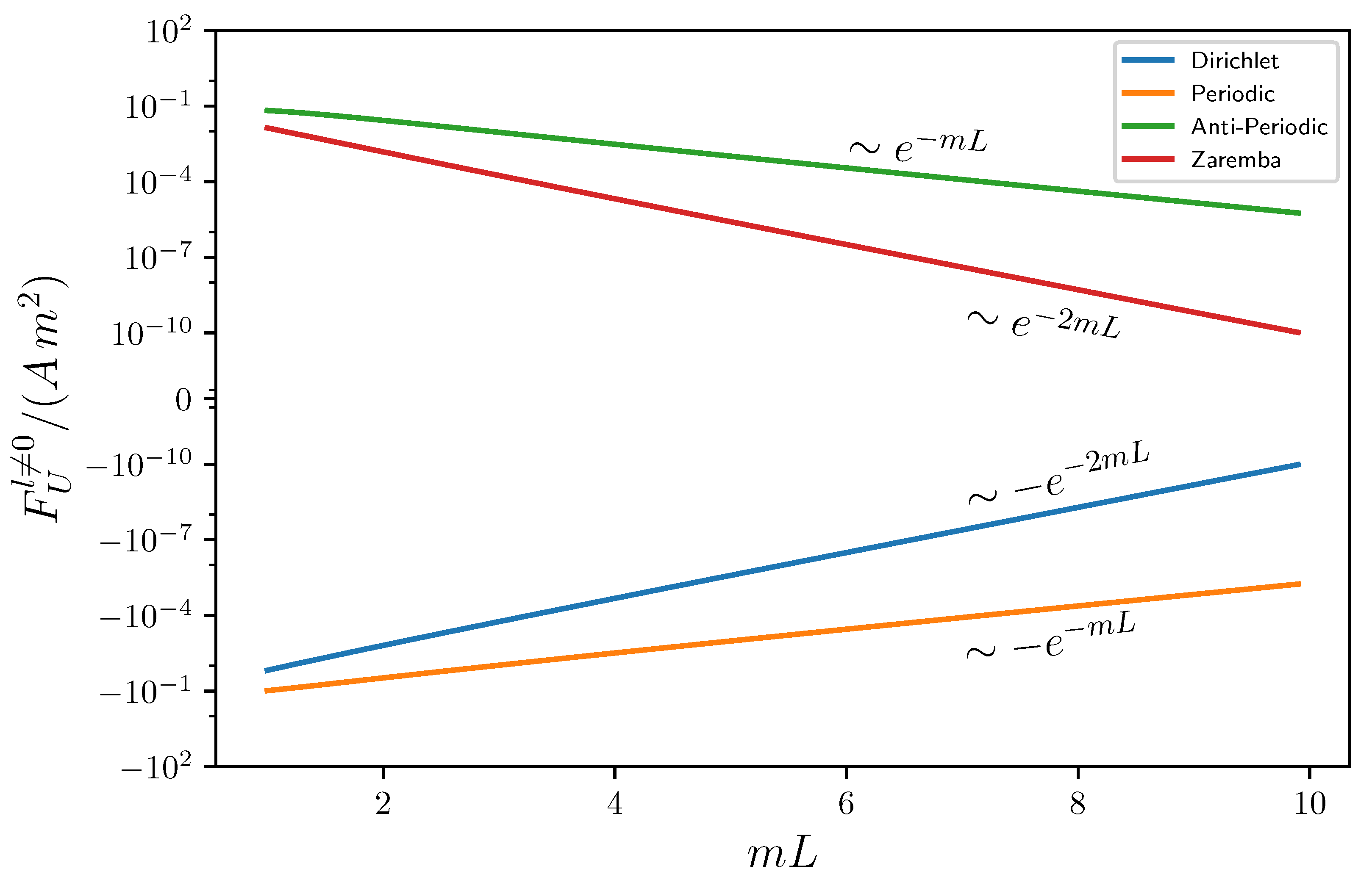
By plotting the temperature-dependent part of the free energy $F_U^{l\ne 0}$ (see Figure 2), it can also be seen how these terms exponentially decay to zero as $mL$ grows.

The physical difference between the two families gives rise to different asymptotic behaviours: the families with faster decays (Dirichlet, Neumann, Zaremba) are conditions imposed on each boundary wire separately, whereas in the second family (periodic, anti-periodic, pseudo-periodic) with slower decay rates, the boundary conditions involve a relationship between the values of the fields in both wires, establishing a interconnection between them.

6. Conclusions

We have shown the existence of two types of boundary conditions which give rise to different regimes of exponential decay of the Casimir energy at large distances for scalar field theories. The two types are distinguished by the feature that the boundary conditions involve or not interconnections between the behaviour of the fields at the two boundaries.

The fast exponential decays of the Casimir energy associated with all massive fields make Casimir energy negligible when compared with the contribution of massless fields coming from electrodynamics. This means that there is no hope of measuring its effects experimentally. However, from a conceptual point of view, it can become of crucial importance to understand the confining infrared behaviour of non-Abelian gauge theories if this regime can be effectively driven by a massive scalar field.

Indeed, analytic arguments [11,12] and non-perturbative numerical simulations [14] show that there is a similar exponential decay in gauge theories with Dirichlet boundary conditions. The verification that such a behaviour is modified for other types of boundary conditions would provide further evidence to the claim that the low-energy behaviours of non-Abelian SU(2) gauge theories are governed by an effective scalar field with a fixed non-vanishing mass. A remarkable feature is that the mass of this scalar field is considerably smaller than the lowest mass of the glueball spectrum [11,12].

In particular, the confirmation of the existence of the two regimes for different boundary conditions will be crucial for the verification of this conjecture. Numerical simulations are in progress to clarify this issue.

References

1. Casimir, H.B.G. On the attraction between two perfectly conducting plates. Proc. Kon. Ned. Akad. Wetensch. B 1948, 51, 793–795. Available online: https://dwc.knaw.nl/DL/publications/PU00018547.pdf (accessed on 22 February 2024).
2. Sparnaay, M.J. Attractive forces between flat plates. Nature 1957, 180, 334–335. [Google Scholar] [CrossRef]
3. Sparnaay, M.J. Measurements of attractive forces between flat plates. Physica 1958, 24, 751–764. [Google Scholar] [CrossRef]
4. Lamoreaux, S.K. Demonstration of the Casimir force in the 0.6 to 6 μm range. Phys. Rev. Lett. 1997, 78, 5–8. [Google Scholar] [CrossRef]
5. Mohideen, U.; Roy, A. Precision measurement of the Casimir force from 0.1 to 0.9 μm. Phys. Rev. Lett. 1998, 81, 4549–4552. [Google Scholar] [CrossRef]
6. Chan, H.B.; Aksyuk, V.A.; Kleiman, R.N.; Bishop, D.J.; Capasso, F. Nonlinear micromechanical Casimir oscillator. Phys. Rev. Lett. 2001, 87, 211801. [Google Scholar] [CrossRef]
7. Dalvit, D.; Milonni, P.; Roberts, D.; da Rosa, F. Casimir Physics; Springer: Berlin/Heidelberg, Germany, 2011. [Google Scholar] [CrossRef]
8. Asorey, M.; Muñoz-Castañeda, J. Attractive and repulsive Casimir vacuum energy with general boundary conditions. Nucl. Phys. B 2013, 874, 852–876. [Google Scholar] [CrossRef]
9. Muñoz-Castañeda, J.; Santamaría-Sanz, L.; Donaire, M.; Tello-Fraile, M. Thermal Casimir effect with general boundary conditions. Eur. Phys. J. C 2020, 80, 793. [Google Scholar] [CrossRef]
10. Symanzik, K. Schrödinger representation and Casimir effect in renormalizable quantum field theory. Nucl. Phys. B 1981, 190, 1–44. [Google Scholar] [CrossRef]
11. Karabali, D.; Nair, V.P. Casimir effect in (2 + 1)-dimensional Yang-Mills theory as a probe of the magnetic mass. Phys. Rev. D 2018, 98, 105009. [Google Scholar] [CrossRef]
12. Karabali, D.; Kim, C.; Nair, V. Planar Yang-Mills theory: Hamiltonian, regulators and mass gap. Nucl. Phys. B 1998, 524, 661–694. [Google Scholar] [CrossRef]
13. Karabali, D.; Nair, V. On the origin of the mass gap for non-Abelian gauge theories in (2 + 1) dimensions. Phys. Lett. B 1996, 1, 141–147. [Google Scholar] [CrossRef]
14. Chernodub, M.N.; Goy, V.A.; Molochkov, A.V.; Nguyen, H.H. Casimir Effect in Yang-Mills Theory in D = 2 + 1. Phys. Rev. Lett. 2018, 121, 191601. [Google Scholar] [CrossRef]
15. Asorey, M.; Ezquerro, F. Energy preserving boundary conditions in field theory. Phys. Rev. D 2023, 4, 045008. [Google Scholar] [CrossRef]
16. Asorey, M.; Beneventano, C.; D’Ascanio, D.; Santangelo, E. Thermodynamics of conformal fields in topologically non-trivial space-time backgrounds. J. High Energy Phys. 2012, 2013, 68. [Google Scholar] [CrossRef]
17. Asorey, M.; Beneventano, C.G.; Cavero-Peláez, I.; D’Ascanio, D.; Santangelo, E.M. Topological entropy and renormalization group flow in 3-dimensional spherical spaces. J. High Energy Phys. 2015, 2015, 78. [Google Scholar] [CrossRef]
18. Zou, J.; Marcet, Z.; Rodriguez, A.W.; Reid, M.T.H.; McCauley, A.P.; Kravchenko, I.I.; Lu, T.; Bao, Y.; Johnson, S.G.; Chan, H.B. Casimir forces on a silicon micromechanical chip. Nat. Commun. 2013, 4, 1845. [Google Scholar] [CrossRef]
19. Terças, H.; Ribeiro, S.; Pezzutto, M.; Omar, Y. Quantum thermal machines driven by vacuum forces. Phys. Rev. E 2017, 95, 022135. [Google Scholar] [CrossRef]
20. Geyer, B.; Klimchitskaya, G.; Mostepanenko, V. Thermal corrections in the Casimir interaction between a metal and dielectric. Phys. Rev. A 2005, 72, 022111. [Google Scholar] [CrossRef]
21. Milton, K.; Kalauni, P.A.; Parashar, P.; Li, Y. Casimir self-entropy of a spherical electromagnetic δ-function shell. Phys. Rev. D 2017, 96, 085007. [Google Scholar] [CrossRef]
22. Bordag, M. Free energy and entropy for thin sheets. Phys. Rev. D 2018, 98, 085010. [Google Scholar] [CrossRef]
23. Asorey, M.; Ibort, A.; Marmo, G. Global theory of quantum boundary conditions and topology change. Int. J. Mod. Phys. A 2005, 20, 1001–1025. [Google Scholar] [CrossRef]
24. Dowker, J.S.; Critchley, R. Effective Lagrangian and energy-momentum tensor in de Sitter space. Phys. Rev. D 1976, 13, 3224–3232. [Google Scholar] [CrossRef]
25. Blau, S.; Visser, M.; Wipf, A. Zeta functions and the Casimir energy. Nucl. Phys. B 1988, 310, 163–180. [Google Scholar] [CrossRef]
26. Moretti, V. Direct ζ-function approach and renormalization of one-loop stress tensors in curved spacetimes. Phys. Rev. D 1997, 56, 7797–7819. [Google Scholar] [CrossRef]
27. Moretti, V. One-loop stress-tensor renormalization in curved background: The relation between ζ-function and point-splitting approaches, and an improved point-splitting procedure. J. Math. Phys. 1999, 40, 3843–3875. [Google Scholar] [CrossRef]
Figure 1. Dependence of the Casimir energy in logarithmic scale as a function of the effective distance m L between the two boundary wires for different boundary conditions.
Physics 06 00040 g001
Figure 2. Free energy behaviour of the temperature-dependent part in logarithmic scale as a function of the effective distance m L between the two boundary wires for different boundary conditions, with m β = 1 .
Physics 06 00040 g002
Disclaimer/Publisher’s Note: The statements, opinions and data contained in all publications are solely those of the individual author(s) and contributor(s) and not of MDPI and/or the editor(s). MDPI and/or the editor(s) disclaim responsibility for any injury to people or property resulting from any ideas, methods, instructions or products referred to in the content.