A Study of Multi-Objective Crashworthiness Optimization of the Thin-Walled Composite Tube under Axial Load


Abstract
1. Introduction
2. Method
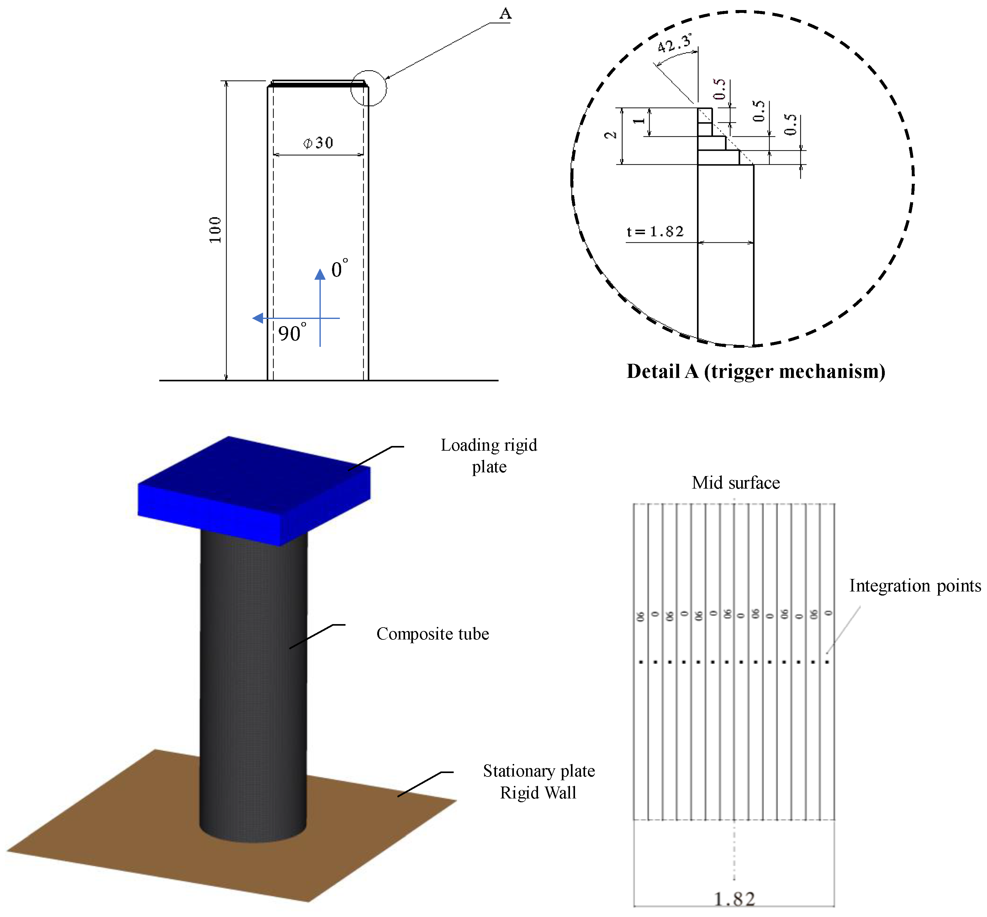
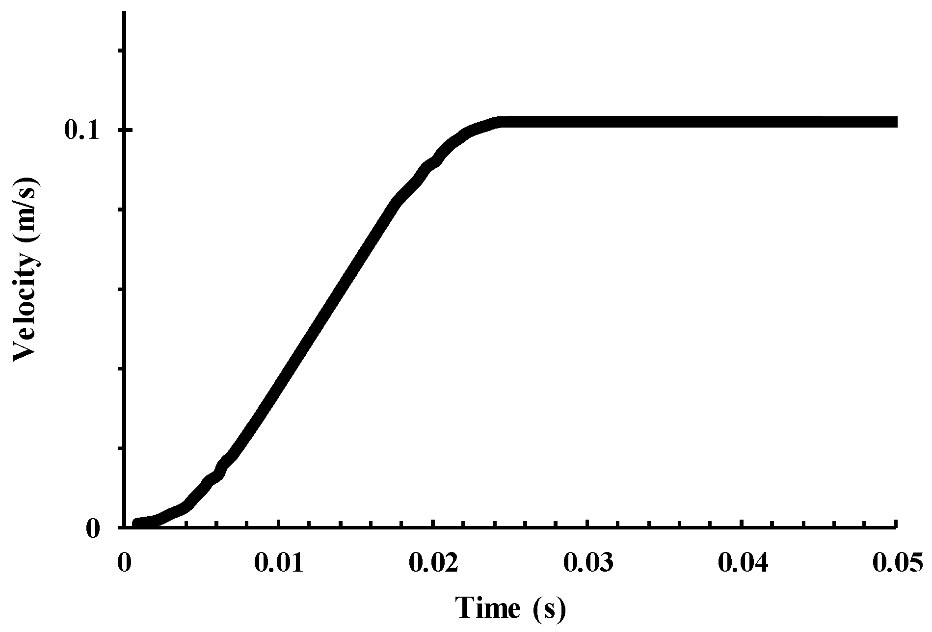
2.1. Finite Element Model
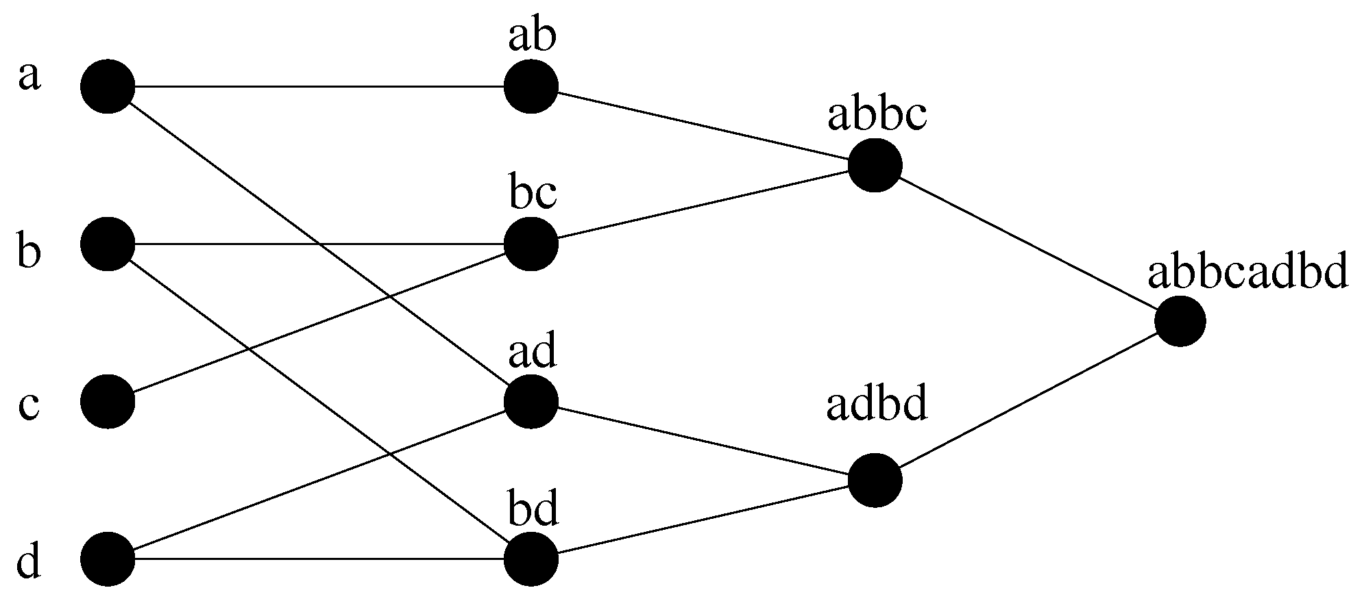
2.2. Modeling Using GMDH Neural Network.
3. Result and Discussion
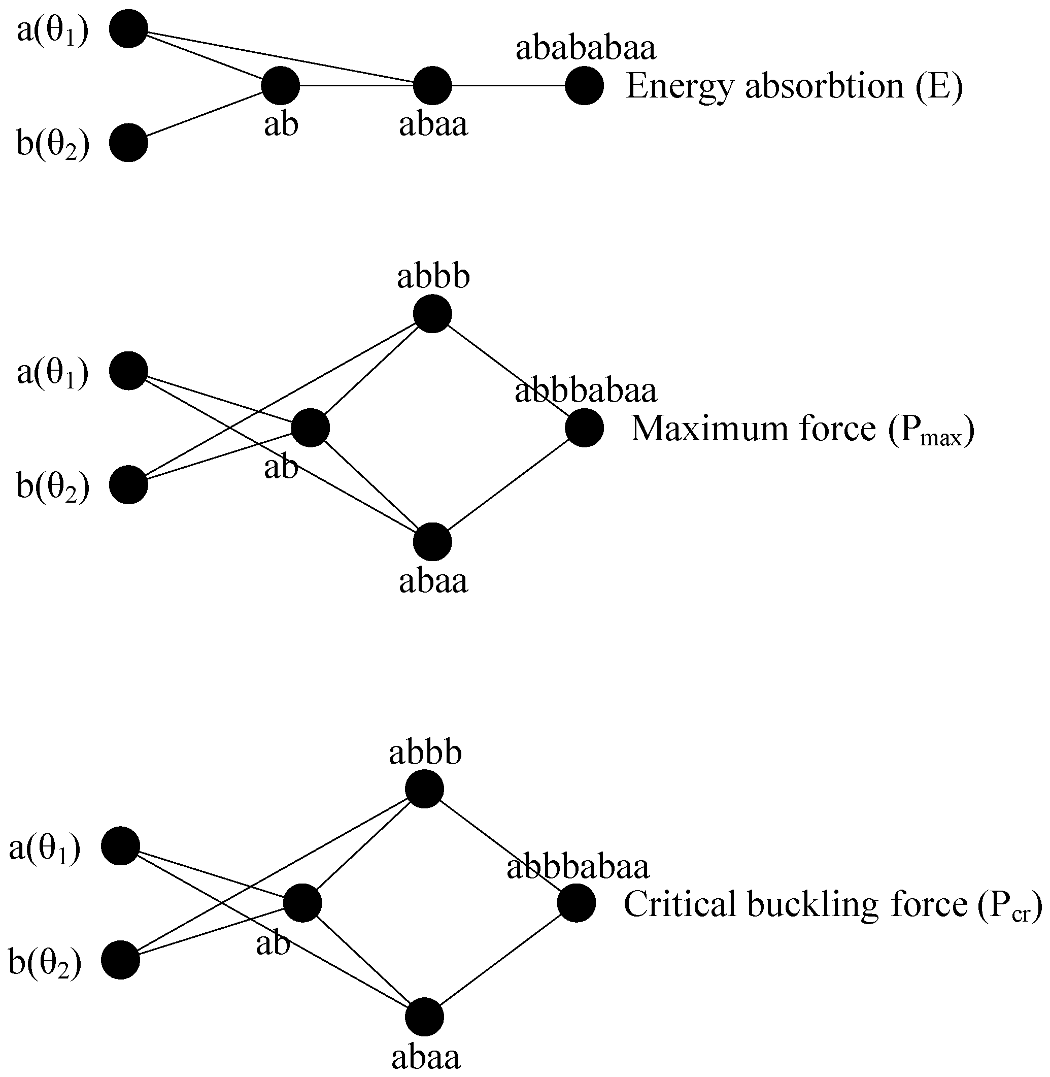
3.1. GMDH Modeling of Crashworthiness Parameters
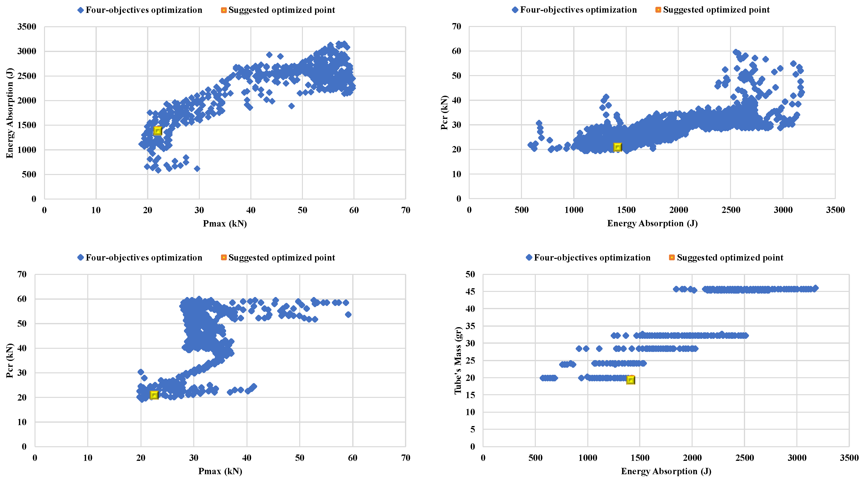
3.2. Multi-Objective Optimization
4. Conclusions
Author Contributions
Funding
Acknowledgments
Conflicts of Interest
Appendix A
References
- Seyedi, M.; Jung, S.; Dolzyk, G.; Wekezer, J. Experimental assessment of vehicle performance and injury risk for cutaway buses using tilt table and modified dolly rollover tests. Accid. Anal. Prev. 2019, 13, 105287. [Google Scholar] [CrossRef] [PubMed]
- Seyedi, M.; Jung, S.; Wekezer, J.; Kerrigan, J.R.; Gepner, B. Rollover Crashworthiness Analyses—An Overview and State of the Art. Int. J. Crashworthiness 2019, 25, 328–350. [Google Scholar] [CrossRef]
- Borazjani, S. Light-weight Design of Vehicle Roof Panel for Stiffness and Crash Analyses. Ph.D. Thesis, Politecnico di Torino, Turin, Italy, 2016. [Google Scholar] [CrossRef]
- Meredith, J.; Bilson, E.; Powe, R.; Collings, E.; Kirwan, K. A performance versus cost analysis of prepreg carbon fibre epoxy energy absorption structures. Compos. Struct. 2015, 124, 206–213. [Google Scholar] [CrossRef]
- Mamalis, A.; Robinson, M.; Manolakos, D.E.; Demosthenous, G.A.; Ioannidis, M.B.; Carruthers, J. Crashworthy capability of composite material structures. Compos. Struct. 1997, 37, 109–134. [Google Scholar] [CrossRef]
- Palanivelu, S.; Van Paepegem, W.; Degrieck, J.; Van Ackeren, J.; Kakogiannis, D.; Van Hemelrijck, D.; Vantomme, J. Experimental study on the axial crushing behaviour of pultruded composite tubes. Polym. Test. 2010, 29, 224–234. [Google Scholar] [CrossRef]
- Mamalis, A.G. Crashworthiness of Composite Thin-Walled Structures; Routledge: London, UK, 2017. [Google Scholar]
- Carruthers, J.J.; Kettle, A.; Robinson, A. Energy Absorption Capability and Crashworthiness of Composite Material Structures: A Review. Appl. Mech. Rev. 1998, 51, 635–649. [Google Scholar] [CrossRef]
- Talib, A.A.; Ali, A.; Badie, M.A.; Lah, N.A.C.; Golestaneh, A.F. Developing a hybrid, carbon/glass fiber-reinforced, epoxy composite automotive drive shaft. Mater. Des. 2010, 31, 514–521. [Google Scholar] [CrossRef]
- Palma, T.; Munther, M.; Damasus, P.; Salari, S.; Beheshti, A.; Davami, K. Multiscale mechanical and tribological characterizations of additively manufactured polyamide 12 parts with different print orientations. J. Manuf. Process. 2019, 40, 76–83. [Google Scholar] [CrossRef]
- Salari, S.; Dadkan, S.; Khakbiz, M.; Atai, M. Effect of Nanoparticles on Surface Characteristics of Dental Nanocomposite. Med. Devices Sens. 2020. [Google Scholar] [CrossRef]
- Caliskan, A.G. Crashworthiness of Composite Materials & Structures for Vehicle Applications. SAE Tech. Pap. 2000, 1, 15. [Google Scholar]
- Gan, N.; Feng, Y.; Yin, H.; Wen, G.; Wang, D.; Huang, X. Quasi-static axial crushing experiment study of foam-filled CFRP and aluminum alloy thin-walled structures. Compos. Struct. 2016, 157, 303–319. [Google Scholar] [CrossRef]
- Belingardi, G.; Boria, S.; Obradovic, J. Energy absorbing sacrificial structures made of composite materials for vehicle crash design. In Dynamic Failure of Composite and Sandwich Structures; Springer: Dordrecht, The Netherlands, 2013; Volume 192, pp. 577–609. [Google Scholar]
- Alkbir, M.; Sapuan, S.M.; Nuraini, A.A.; Ishak, M.R. Fibre properties and crashworthiness parameters of natural fibre-reinforced composite structure: A literature review. Compos. Struct. 2016, 148, 59–73. [Google Scholar] [CrossRef]
- Kazancı, Z.; Bathe, K.-J. Crushing and crashing of tubes with implicit time integration. Int. J. Impact Eng. 2012, 42, 80–88. [Google Scholar] [CrossRef]
- Huang, J.; Wang, X. Numerical and experimental investigations on the axial crushing response of composite tubes. Compos. Struct. 2009, 91, 222–228. [Google Scholar] [CrossRef]
- Swaminathan, N.; Averill, R.C. Contribution of failure mechanisms to crush energy absorption in a composite tube. Mech. Adv. Mater. Struct. 2006, 13, 51–59. [Google Scholar] [CrossRef]
- Bank, L.C. Progressive failure and ductility of FRP composites for construction. J. Compos. Constr. 2013, 17, 406–419. [Google Scholar] [CrossRef]
- Farley, G.L.; Jones, R.M. Prediction of the Energy-Absorption Capability of Composite Tubes. J. Compos. Mater. 1992, 26, 388–404. [Google Scholar] [CrossRef]
- Israr, H.A.; Rivallant, S.; Bouvet, C.; Barrau, J.J. Finite element simulation of 0/90 CFRP laminated plates subjected to crushing using a free-face-crushing concept. Compos. Part A Appl. Sci. Manuf. 2014, 62, 16–25. [Google Scholar] [CrossRef]
- Jia, X.; Chen, G.; Yu, Y.; Li, G.; Zhu, J.; Luo, X.; Duan, C.; Yang, X.; Hui, D. Effect of geometric factor, winding angle and pre-crack angle on quasi-static crushing behavior of filament wound CFRP cylinder. Compos. Part B Eng. 2013, 45, 1336–1343. [Google Scholar] [CrossRef]
- Palanivelu, S.; Van Paepegem, W.; Degrieck, J.; Kakogiannis, D.; Van Ackeren, J.; Van Hemelrijck, D.; Wastiels, J.; Vantomme, J. Parametric study of crushing parameters and failure patterns of pultruded composite tubes using cohesive elements and seam, Part. I: Central delamination and triggering modelling. Polym. Test. 2010, 29, 729–741. [Google Scholar] [CrossRef]
- Alghamdi, A. Collapsible impact energy absorbers: An. overview. Thin-walled Struct. 2001, 39, 189–213. [Google Scholar] [CrossRef]
- Xiao, X. Evaluation of a composite damage constitutive model for PP composites. Compos. Struct. 2007, 79, 163–173. [Google Scholar] [CrossRef]
- Xiao, X.; Botkin, M.E.; Johnson, N.L. Axial crush simulation of braided carbon tubes using MAT58 in LS-DYNA. Thin-Walled Struct. 2009, 47, 740–749. [Google Scholar] [CrossRef]
- Wade, B.; Feraboli, P.; Osborne, M. Simulating Laminated Composites Using LS-DYNA Material Model MAT54 Part I:[0] and [90] Ply Single-Element Investigation; FAA JAMS: Baltimore, MD, USA, 2012. [Google Scholar]
- Curtis, J.; Hinton, M.J.; Li, S.; Reid, S.R.; Soden, P.D. Damage, deformation and residual burst strength of filament-wound composite tubes subjected to impact or quasi-static indentation. Compos. Part B Eng. 2000, 31, 419–433. [Google Scholar] [CrossRef]
- Song, S.; Waas, A.M.; Shahwan, K.W.; Xiao, X.; Faruque, O. Braided textile composites under compressive loads: Modeling the response, strength and degradation. Compos. Sci. Technol. 2007, 67, 3059–3070. [Google Scholar] [CrossRef]
- Zarei, H.; Kröger, M.; Albertsen, H. An experimental and numerical crashworthiness investigation of thermoplastic composite crash boxes. Compos. Struct. 2008, 85, 245–257. [Google Scholar] [CrossRef]
- Nariman-Zadeh, N.; Darvizeh, A.; Ahmad-Zadeh; Hybrid, G. Genetic design of GMDH-type neural networks using singular value decomposition for modelling and prediction of the explosive cutting process. Mech. Eng. Part B J. Eng. Manuf. 2003, 217, 779–790. [Google Scholar] [CrossRef]
- Nariman-Zadeh, N.; Darvizeh, A.; Felezi, E.M.; Gharababaei, H. Polynomial modelling of explosive compaction process of metallic powders using GMDH-type neural networks and singular value decomposition. Model. Simul. Mater. Sci. Eng. 2002, 10, 727. [Google Scholar] [CrossRef]
- Amanifard, N.; Nariman-Zadeh, N.; Borji, M.; Khalkhali, A.; Habibdoust, A. Modelling and Pareto optimization of heat transfer and flow coefficients in microchannels using GMDH type neural networks and genetic algorithms. Energy Convers. Manag. 2008, 49, 311–325. [Google Scholar] [CrossRef]
- Khalkhali, A.; Safikhani, H. Pareto based multi-objective optimization of a cyclone vortex finder using CFD, GMDH type neural networks and genetic algorithms. Eng. Optim. 2012, 44, 105–118. [Google Scholar] [CrossRef]
- Ivakhnenko, A.G. Polynomial theory of complex systems. IEEE Trans. Syst. Man Cybern. 1971, 1, 364–378. [Google Scholar] [CrossRef]
- Atashkari, K.; Nariman-Zadeh, N.; Gölcü, M.; Khalkhali, A.; Jamali, A. Modelling and multi-objective optimization of a variable valve-timing spark-ignition engine using polynomial neural networks and evolutionary algorithms. Energy Convers. Manag. 2007, 48, 1029–1041. [Google Scholar] [CrossRef]
- Kim, J.-S.; Yoon, H.-J.; Shin, K.-B. A study on crushing behaviors of composite circular tubes with different reinforcing fibers. Int. J. Impact Eng. 2011, 38, 198–207. [Google Scholar] [CrossRef]
- Tsai, S.W.; Wu, E.M. A general theory of strength for anisotropic materials. J. Compos. Mater. 1971, 5, 58–80. [Google Scholar] [CrossRef]
- Du Bois, P.; Chou, C.C.; Fileta, B.B.; Khalil, T.B.; King, A.I.; Mahmood, H.F.; Mertz, H.J.; Wismans, J.; Prasad, P.; Belwafa, J.E. Vehicle Crashworthiness and Occupant Protection; American Iron and Steel Institute: Detroit, MI, USA, 2004. [Google Scholar]
- Atashkari, K.; Nariman-Zadeh, N.; Pilechi, A.; Jamali, A.; Yao, X. Thermodynamic Pareto optimization of turbojet engines using multi-objective genetic algorithms. Int. J. Therm. Sci. 2005, 44, 1061–1071. [Google Scholar] [CrossRef]


| Mechanical Properties | Carbon/Epoxy | Epoxy Resin |
|---|---|---|
| Tensile modulus (GPa) | 130 (11.4) * | 3.4 |
| Tensile strength (MPa) | 2725 (78.0) | 37.5 |
| Compressive modulus (GPa) | 91.7 (19.2) | NA |
| Compressive strength (MPa) | 551.2 (69.4) | NA |
| Shear modulus (GPa) | 8.2 (0.2) | 2.1 |
| Shear strength (MPa) | 78.4 (3.1) | 36.1 |
| ILSS (MPa) | 71.0 (0.3) | NA |
| Parameter | Value |
|---|---|
| DFAILT | 0.01 |
| DFAILC | −0.013 |
| DFAILM | 0.03 |
| DFAILS | 0.01 |
| Test | Mean Force (Pm-kN) | Maximum Force (Pmax-kN) | Specific Energy Absorption (SEA -kJ/kg) |
|---|---|---|---|
| Numerical simulation | 25.8 | 35.4 | 73.4 |
| Experimental analysis [37] | 25.2 | 31.4 | 72.7 |
| Simulation Number | Input Data | Output Data | ||||||
|---|---|---|---|---|---|---|---|---|
| E (J) | Pmax (kN) | Pcr (kN) | ||||||
| θ1 (deg) | θ2 (deg) | FEM | GMDH | FEM | GMDH | FEM | GMDH | |
| 1 | 90 | 180 | 2567 | 2535 | 43 | 41.8 | 42 | 42.5 |
| 2 | 90 | 135 | 1982 | 1991 | 27 | 27.8 | 30 | 30.7 |
| 3 | 90 | 90 | 2083 | 2096 | 30 | 26.9 | 31 | 29.3 |
| 4 | 90 | 45 | 1982 | 1986 | 27 | 27.9 | 30 | 30.6 |
| 5 | 90 | 0 | 2568 | 2612 | 43 | 43.9 | 43 | 43.6 |
| 6 | 60 | 180 | 1928 | 1825 | 34 | 32.1 | 34 | 33.1 |
| 7 | 60 | 160 | 1380 | 1437 | 23 | 26.3 | 26 | 27.7 |
| 8 | 60 | 45 | 1202 | 1215 | 22 | 22.2 | 24 | 23.9 |
| 9 | 60 | 0 | 1928 | 1914 | 34 | 33.3 | 34 | 33.6 |
| 10 | 30 | 135 | 1015 | 1047 | 20 | 19.2 | 20 | 19.82 |
| 11 | 30 | 45 | 1055 | 1074 | 19 | 19.3 | 19 | 18.9 |
| 12 | 0 | 135 | 1437 | 1372 | 37 | 36.9 | 37 | 36.9 |
| 13 | 0 | 45 | 1435 | 1395 | 37 | 38.2 | 37 | 37.1 |
| Output Parameter | RMSE | R2 | MAPE |
|---|---|---|---|
| Absorbed energy (E) | 18.7 | 0.99 | 2.22 |
| Maximum force (Pmax) | 0.79 | 0.99 | 1.02 |
| Critical force (Pcr) | 1.51 | 0.99 | 2.48 |
| Model | Optimized Outputs | ||
|---|---|---|---|
| SEA (kJ/kg) | Pmax (kN) | Pcr (kN) | |
| GMDH neural network | 72.6 | 23.7 | 21.08 |
| Numerical FE simulation | 68.5 | 23 | 23.03 |
| Error | 5.6 | 3 | 9.2 |
© 2020 by the authors. Licensee MDPI, Basel, Switzerland. This article is an open access article distributed under the terms and conditions of the Creative Commons Attribution (CC BY) license (http://creativecommons.org/licenses/by/4.0/).
Share and Cite
Seyedi, M.R.; Khalkhali, A. A Study of Multi-Objective Crashworthiness Optimization of the Thin-Walled Composite Tube under Axial Load. Vehicles 2020, 2, 438-452. https://doi.org/10.3390/vehicles2030024
Seyedi MR, Khalkhali A. A Study of Multi-Objective Crashworthiness Optimization of the Thin-Walled Composite Tube under Axial Load. Vehicles. 2020; 2(3):438-452. https://doi.org/10.3390/vehicles2030024
Chicago/Turabian StyleSeyedi, Mohammad Reza, and Abolfazl Khalkhali. 2020. "A Study of Multi-Objective Crashworthiness Optimization of the Thin-Walled Composite Tube under Axial Load" Vehicles 2, no. 3: 438-452. https://doi.org/10.3390/vehicles2030024
APA StyleSeyedi, M. R., & Khalkhali, A. (2020). A Study of Multi-Objective Crashworthiness Optimization of the Thin-Walled Composite Tube under Axial Load. Vehicles, 2(3), 438-452. https://doi.org/10.3390/vehicles2030024