Numerical Study of Longitudinal Inter-Distance and Operational Characteristics for High-Speed Capsular Train Systems

Abstract

High-speed capsular vehicles are firstly suggested as an idea by Elon Musk of Tesla Company. Unlike conventional high-speed trains, capsular vehicles are individual vessels carrying passengers and freight with the expected maximum speed of near 1200 [km/h] in a near-vacuum tunnel. More individual vehicle speed, dispatch, and position control in the operational aspect are expected over connected trains. This numerical study and investigation evaluate and analyze inter-distance control and their characteristics for high-speed capsular vehicles and their operational aspects. Among many aspects of operation, the inter-distance of multiple vehicles is critical toward passenger/freight flow rate and infrastructural investment. In this paper, the system’s equation, equation of the motion, and various characteristics of the system are introduced, and in particular control design parameters for inter-distance control and actuation are numerically shown. As a conclusion, (1) Inter-distance between vehicles is a function of error rate and second car start time, the magnitude range is determined by second car start time, (2) Inter-distance fluctuation rate is a function of error rate and second car start time, however; it can be minimized by choosing the correct second car start time, and (3) If the second car start time is chosen an integer number of push-down cycle time at specific velocity error rate, the inter-distance fluctuation can be zero.

1. Introduction

The conventional modes of transportation of people consist of four unique types and that are rail, road, water, and air. As transportation technology has been advanced in recent years, people are seeking much faster and more efficient ground transportation ways all over the world. Many countries have developed high-speed railway transportation. The most famous one is the Chinese bullet train- China Railway High-speed(CRH) train series as shown in Figure 1. with a normal speed of 350 [km/h], and now the Shanghai Maglev can reach a speed of 430 [km/h] during daily operation [1]. Other countries like France has SNCF TGV series train with a speed of 350 [km/h], Japan has Shinkansen series train with a speed of 320 [km/h], Germany has ICE with 320 [km/h], Spain AVE with 310 [km/h], South Korea KTX train with 305 [km/h], etc. [2,3,4,5].

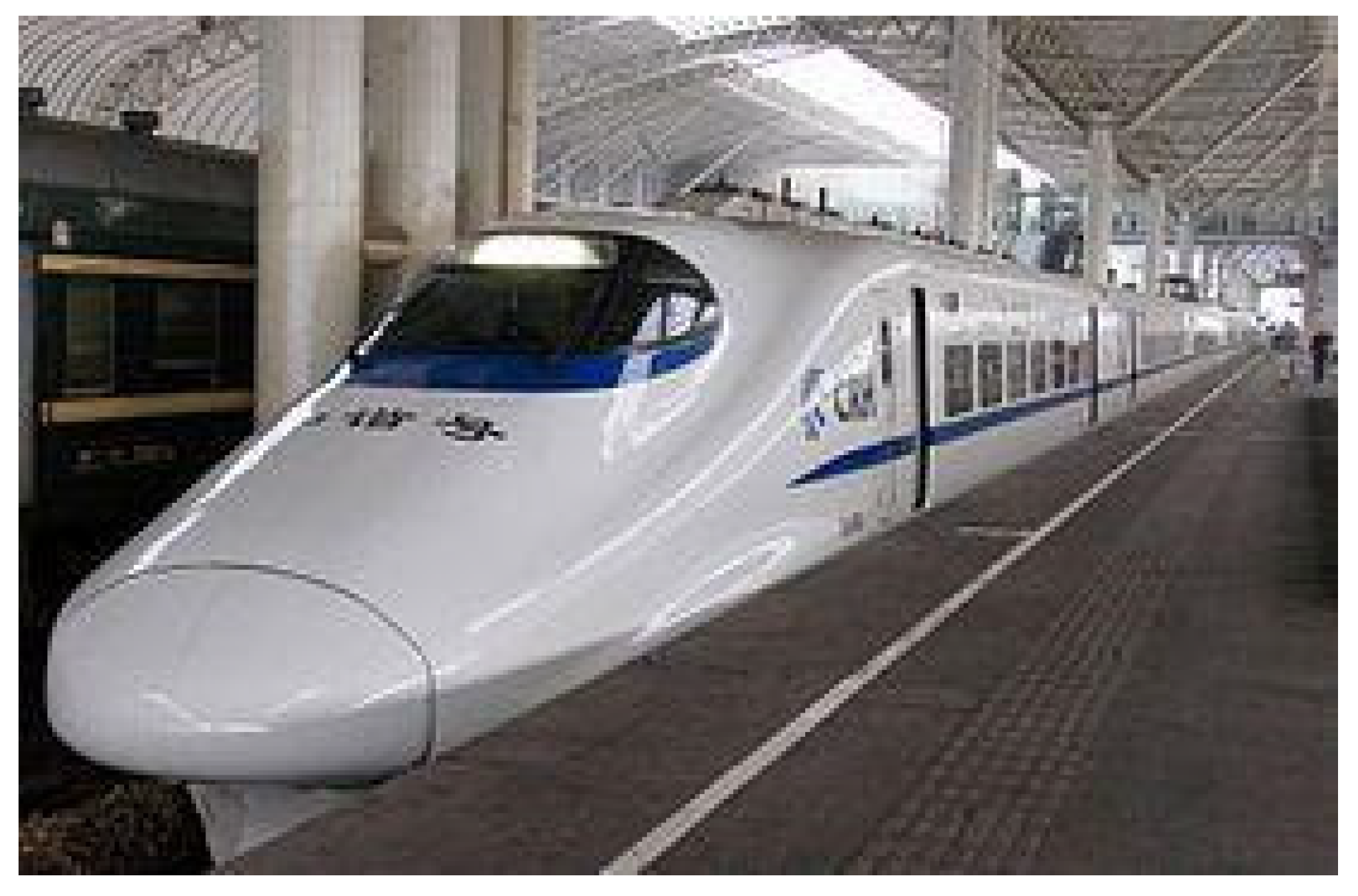
2. High-Speed Capsular Vehicles and Related Works

High-speed capsular systems are vehicles that travel within a vacuumed tunnel, which is designed to travel a long distance within a very short time. Due to reduced aerodynamic resistance, the vehicles normally can travel at ultra-high speed, more than 1000 [km/h]. The transportation system departures with a passenger-vehicle capsule pod as depicted in Figure 2. Hyperloop is one of the high-speed capsular vehicles, which was first published by Elon Musk of Tesla Company in August 2013 [6,7,8,9,10]. It is a kind of vehicle system incorporating reduced-pressure tubes in which pressurized capsules ride on air bearings driven by linear induction motors and axial compressors [11,12,13]. Reduced air resistance could permit vactrains to travel at very high speeds with relatively little power. Unlike conventional high-speed trains, capsular vehicles are individual vessels carrying passengers and freight with the expected maximum speed of near 1200 [km/h] in a near-vacuum tunnel and CFD (Computational fluid dynamics) works have been performed to validate feasibilities [14,15,16]. Capsular vehicles have a lot of advantages over traditional on-ground transportations like high speed, capacity, fuel efficiency, operational cost, environmentally friendly, etc. [17,18,19]. Among various subject areas for realization including communication [20,21], software systems and their designs [22], performance modeling and simulations [23], energy management [24] and eco-friendly effect [25], train control management and operation [26,27,28], this paper focuses on the inter-distance control aspect in operation since its inter-distance is directly related to the number of passengers, freight, and the overall efficacy of hyperloop system operation.

M. Overton et al. focused on and described the capsule hazards and mitigations along with specialized evacuation processes appropriate for Hyperloop [29]. C. Taylor et al. did a high-level Hyperloop commercial feasibility analysis overview about system costs, market, safety, capacity, etc. [30]. K. Goeverden et al. did Hyperloop performance analysis and comparison with high-speed rail and air passenger transport system about the operation, finance, and environment, found out that Hyperloop is better for the environment with long-distance travel, but not for operation and finance [31]. Mitropoulos and et al. did a construction design about the Hyperloop transportation system. They proposed the model of the tube, capsule, compressor, suspension, and propulsion [32]. The MIT Hyperloop Team and some academic institutes competed in the SpaceX Hyperloop competition from June 2015 to January 2017 [17,33]. They did a detailed explanation of the design of the pod, the construction of the pod, and the tests that were performed–including an analysis of the competition run.

R. Janzen proposed a high-speed vehicle model–Transpod. It is designed to carry passengers at speeds exceeding 1000 [km/h], presented concerning dynamics considerations. The system is based on electromagnetic propulsion of vehicles within a protected tube guideway, whose air pressure is reduced and controlled for improved performance at high speed. The tube environment is designed for levitation systems, stability systems, and safety support systems, to permit multiple TransPod vehicles to run simultaneously with high-frequency departures [12].

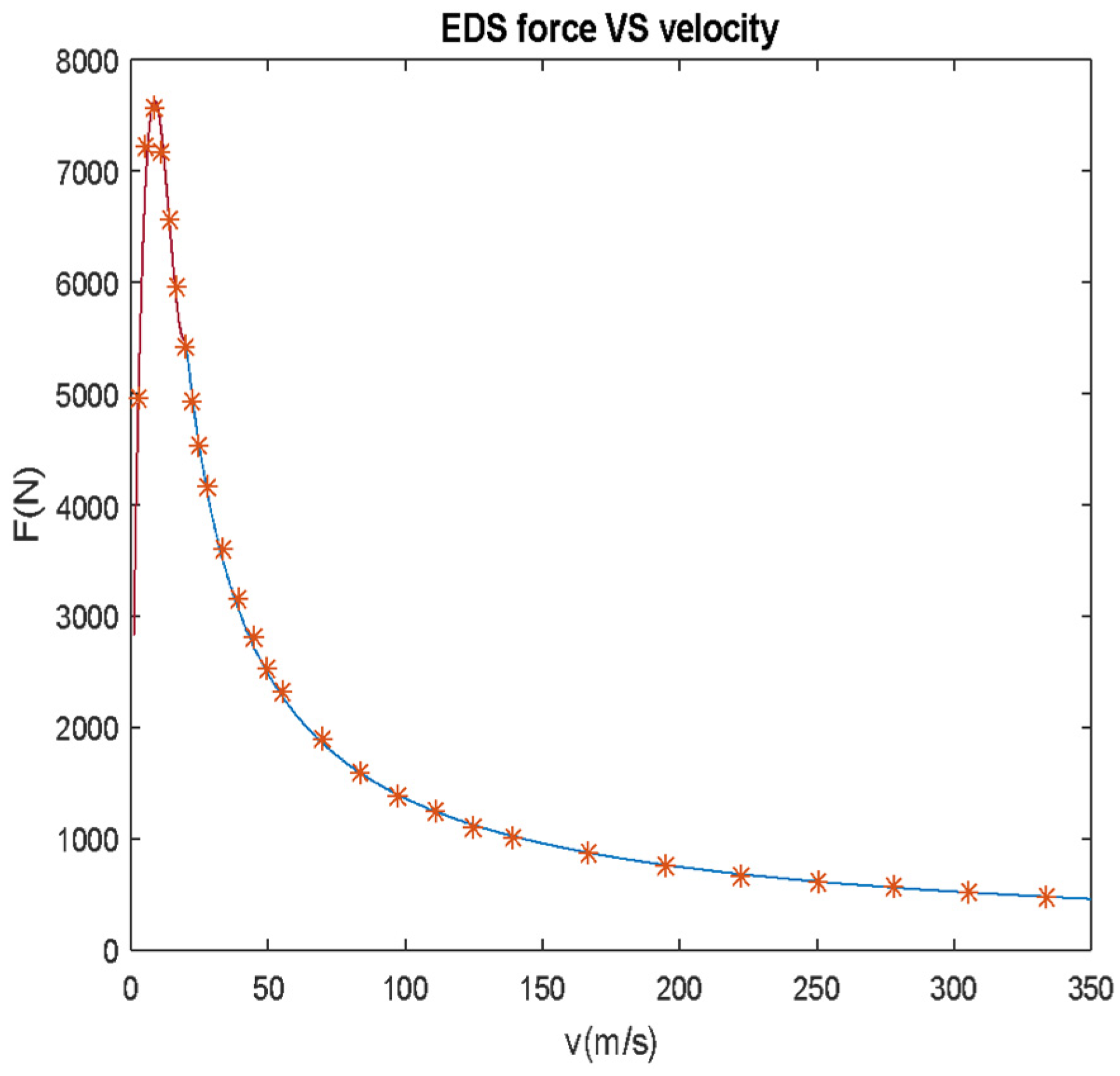
3. Systems Dynamic Model

In this paper, a specific system model and its specification has been used as shown in

Table 1. Given System Specifications.

Given System Specifications
Pressure	1/1000 [atm]
Max speed	1220 [km/h] (339 [m/s])
Weight	24,000 [kg] (No passenger)
	26,000 [kg] (with full passenger)
Dimension	1.25 × 1.25 × 26 [m3]
Levitation gap	over 100 [mm]
Levitation	Superconductor EDS
Propulsion	LSM
Acceleration	(+,−) 0.5 g [m/(s^2)]

. Traffic dynamics modeling is an essential task for longitudinal control. For single-lane traffic modeling, considering constant space platoon, the dynamics function will be defined:

$$X_i=X_{i-1}-D_i$$

(1)

where $X_{i-1}$ and $X_i$ are the x (longitudinal axis) co-ordinates of the preceding vehicle and the vehicle under the consideration and $D_i$ is a constant distance between adjacent two vehicles. For single-vehicle dynamic modeling,

$$m\ddot{X}={\displaystyle \sum }\hspace{1em}\hspace{1em}F\left(t\right)=F_{input}\left(t\right)-F_d-F_{EDS}$$

(2)

Aero resistance force $F_d$ is

$$F_d=C_D\times \frac{1}{2}\times \rho \times V^2\times A\left(N\right)$$

(3)

where:

$$\rho =0.00116 \mathrm{kg}/{\mathrm{m}}^3,$$

$$C_D=6.5,A=1.41 {\mathrm{m}}^2,Fd=0.0053{\mathrm{V}}^2.$$

EDS resistance force is a resistance force caused by magnetic levitation. We obtained experimental data of the real-time EDS force corresponding to a series of velocities from 0 [km/h] to 1220 [km/h]. Using the discrete data, we generated the continuous equation to simulate the data set, which is given by Equation (4). To better illustrate the proximity of the equation, we draw the trend line of the data set as shown in Figure 3 below.

In this system, the aerodynamic drag force and EDS resistance force are both functions of velocity. Thus, the system equation can become:

$$m\dot{V}=F_{input}\left(t\right)-F_d\left(V\right)-F_{EDS}\left(V\right)$$

(4)

Furthermore, we have:

$$\dot{V}=F_{input}\left(t\right)/m-F_d\left(V\right)/m-F_{EDS}\left(V\right)/m$$

(5)

If the input force is given always proportional to the mass, then the system becomes a first-ordinary differential equation about velocity no matter how much the system masses are. Thus, to solve this system is to solve the velocity of this system.

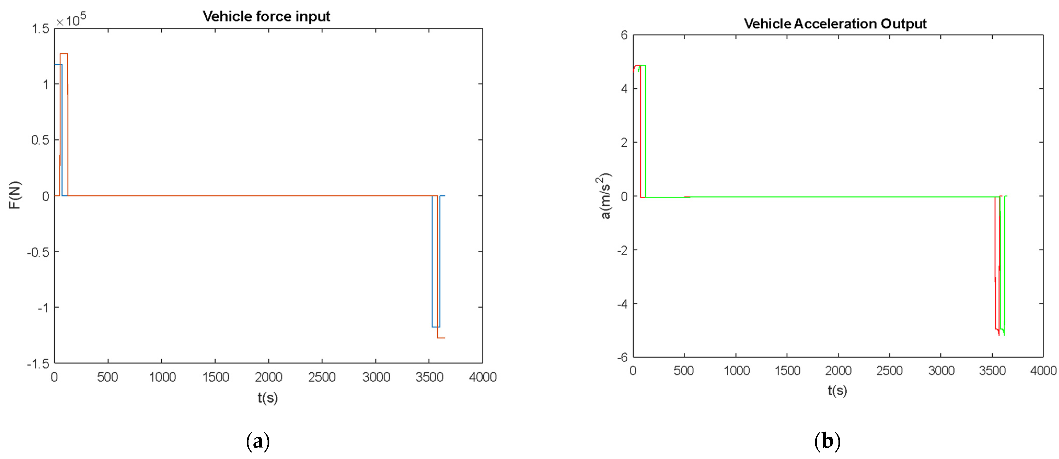
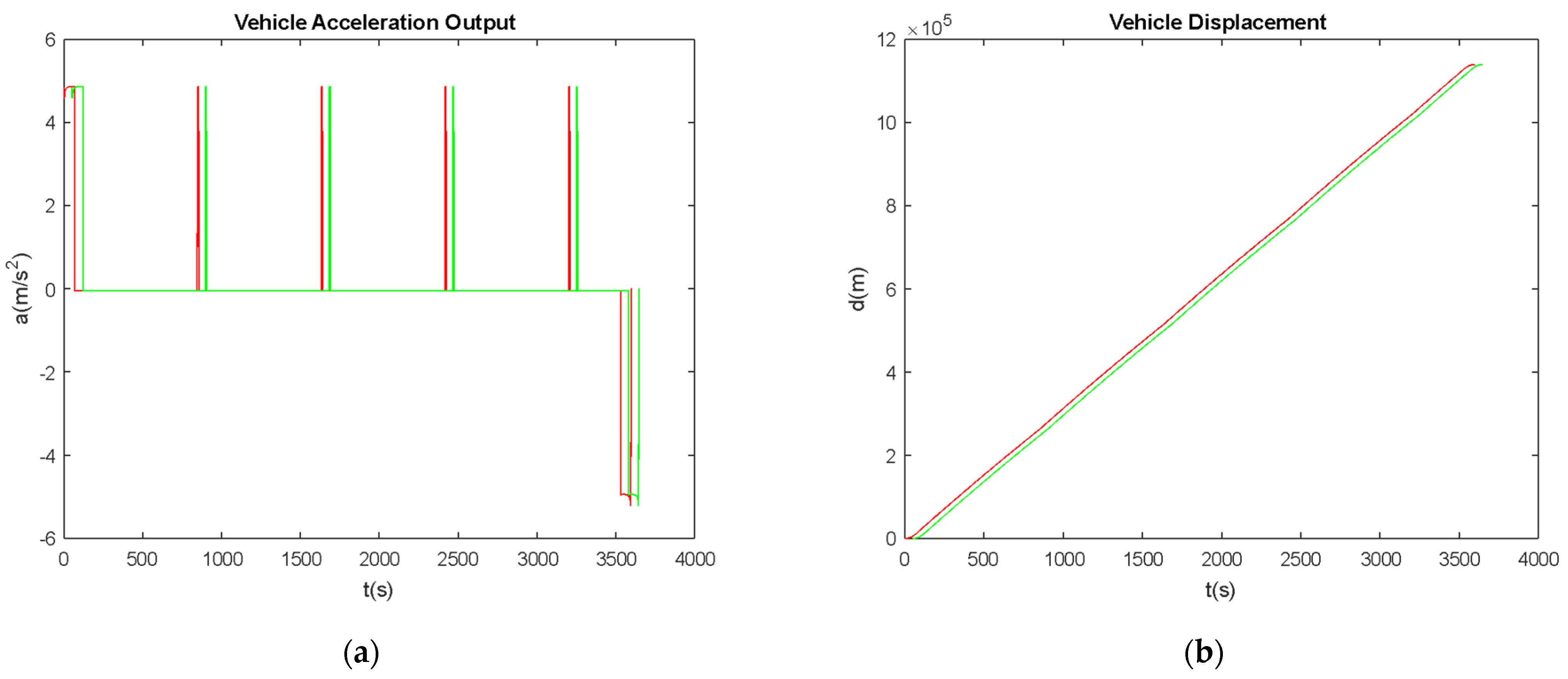
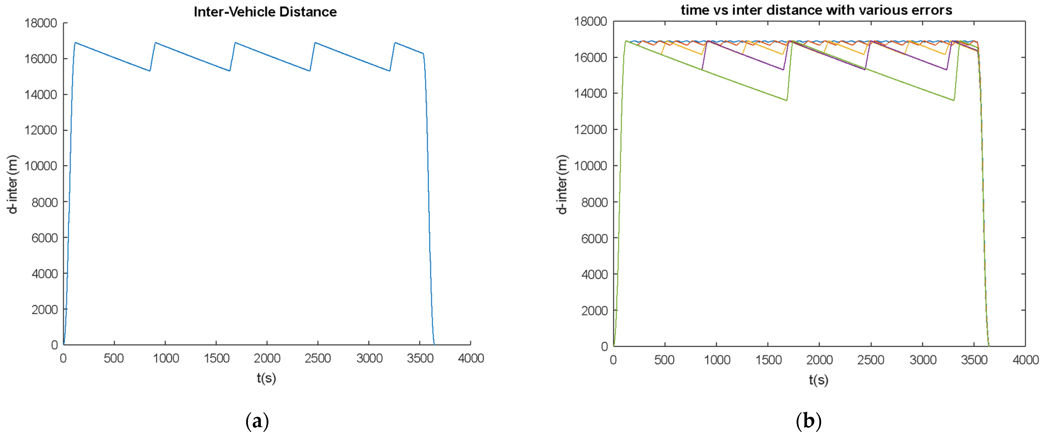
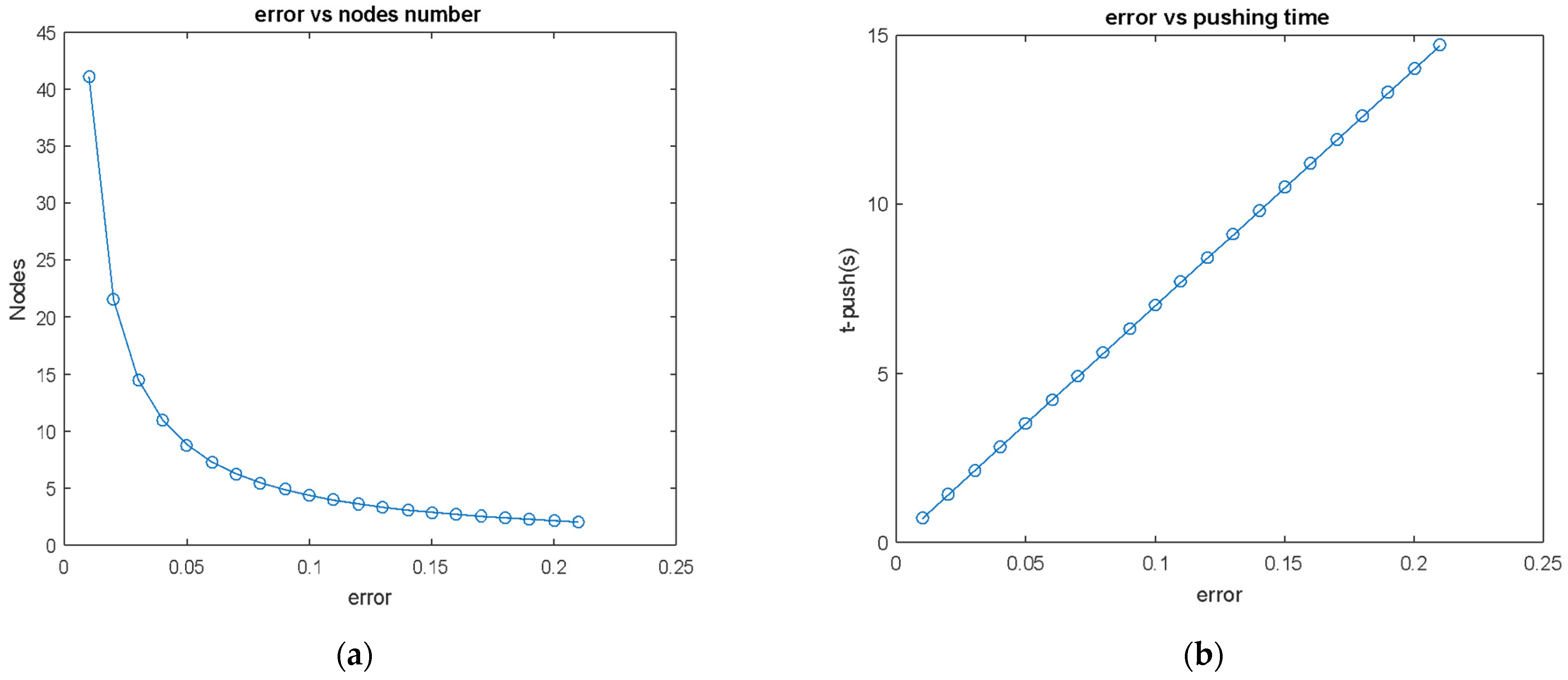
4. Numerical Analysis

In our simulation, the mass is given by two states: 24,000 [kg] with no load and 26,000 [kg] with a full load. We assume in this system two vehicles are departing at a certain time, first with no load and second with a full load. At first, to make the system simple and efficient, we give a pulse force denoted in Figure 4a. Then the vehicles’ acceleration output response is shown in Figure 4b. For the first vehicle, if we give the initial input force to push the vehicle to maximum speed, then stop pushing, let the vehicle drive freely in the tunnel, after a certain time, give the same negative force to decelerate, and we name these three regions as acceleration region, free region, and deceleration region. As you can see, for the corresponding velocity figure, the acceleration region, the speed is increasing rapidly with an acceleration of about 4.9 [m/s^2], for the free drop region, the speed is slowly dropping, due to there is not a lot of resistance, the deceleration is small, for the deceleration region, the speed is decreasing sharply. The second car starts 50 [s] later and is given the same force pattern. The acceleration output response of the second vehicle is the same as the first one.

As shown in Figure 4b, two vehicles’ acceleration outputs are having the same pattern—acceleration-slow dropping-deceleration. Figure 5a shows the acceleration region, as the velocity goes up before 19.82 [m/s], the acceleration is decreasing a little, and after the velocity passes the 19.82 [m/s], the EDS force goes down, the acceleration goes up to the about 4.9 [m/s^2]. Figure 5b shows for the constant but deceleration region due to aerodynamic drag and EDS resistance, the velocity is dropping at an acceleration of −0.04 [m/s^2]. For the deceleration region shown in Figure 6a, the absolute value of deceleration is increasing as the velocity goes down. Figure 6b shows the corresponding velocity response of two vehicles where 50 [s] is apart from the start time.

Another important aspect of the capsular vehicle’s operation is its inter-distance or displacement. The displacement of two vehicles is shown in Figure 7a. They are having the same nonlinear pattern with a time difference of 50 [s]. The inter-distance between two vehicles is changing as the figure shows in Figure 7b. Inter-distance is a nonlinear pattern. Inter-distance is going up quickly up to maximum at first 120 [s], then it starts dropping gradually because the speed of the first vehicle is smaller than the second one, finally, it drops rapidly to zero at the end.

The inter-distance is changing a lot in the middle region. However, from a system stability view, this is not good, thus we need to control the inter-distance to a proper range.

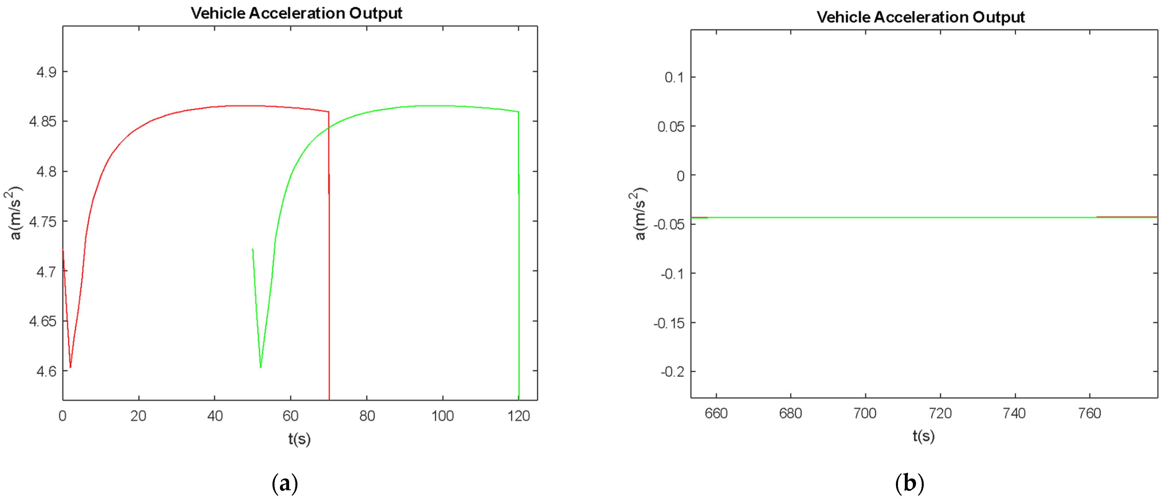
5. Vehicle’s Actuation and Operation Aspects

To control the inter-distance, we need to adjust the two vehicles’ displacement. Then we will need to regulate the vehicle velocity. We have two choices—either we control the single-vehicle velocity pattern or adjust the second car start time. To make our system more stable, we are trying to give the input during the free drop region for a single vehicle. We introduced the velocity drop error, which is defined by:

$$Error=\left(Vmax-Vmin\right)/Vmax$$

(6)

where $Vmax$ is the designed maximum speed, $Vmin$ is the free drop minimum speed allowance, and $Error$ is the speed drop allowance;

From this design, first, we push the vehicle to the maximum. When the velocity dropped to a certain speed, we give one input to push the vehicle speed back to maximum and then let it go freely. When the speed drops to the allowed minimum again and we give the push again, then keep doing the same loop until it gets to the final deceleration region.

Figure 8a shows a velocity response with an error of 0.1. In this case, the maximum speed is 339 [m/s], then the minimum speed allowance is 305.1 [m/s]. Whenever the velocity dropped down to 305.1 [m/s], the vehicle will get a push to 339 [m/s]. Then the designed input force for this scenario is shown in Figure 8b. For two vehicles with different masses, the force impulses are 118 [KN] and 128 [KN] separately.

Then the vehicle output acceleration is shown in Figure 9a. For the acceleration and deceleration region, the acceleration output is the same as without regulation. For the middle region, the acceleration gets the same positive pulses when the input force has functioned.

The vehicle’s displacement is shown in Figure 10a. The trend is the same as before. Figure 10a shows the inter-distance after regulation, as we see, the inter-distance is get controlled in one range, which means the velocity control is effective. However, it is getting multi up-down regions. Moreover, various error rates were applied as shown in Figure 10b.

5.1. Minimizing the Flunctuation Distance

To minimize the inter-distance fluctuation range, we are going to try two ways: (1) control the velocity error, and (2) control the second car start time. First, we fix the second vehicle start time at 50 [s] and vary the velocity error. Figure 10b shows the inter-distance with various errors at 1%, 2%, 5%, 10%, 20%. Inter-distance fluctuation is increasing when the error increases.

For one up-down region, we name it a node. As we see in Figure 11a, the nodes number is decreasing exponentially when the error increases. Moreover, the pushing time for pushing vehicles back to maximum speed from minimum is increasing linearly when error increases, see Figure 11b. The inter-distance fluctuation (df), which refers to the difference of maximum value and minimum value of fluctuation region, is also increasing linearly when error increases, also shown in Figure 11b.

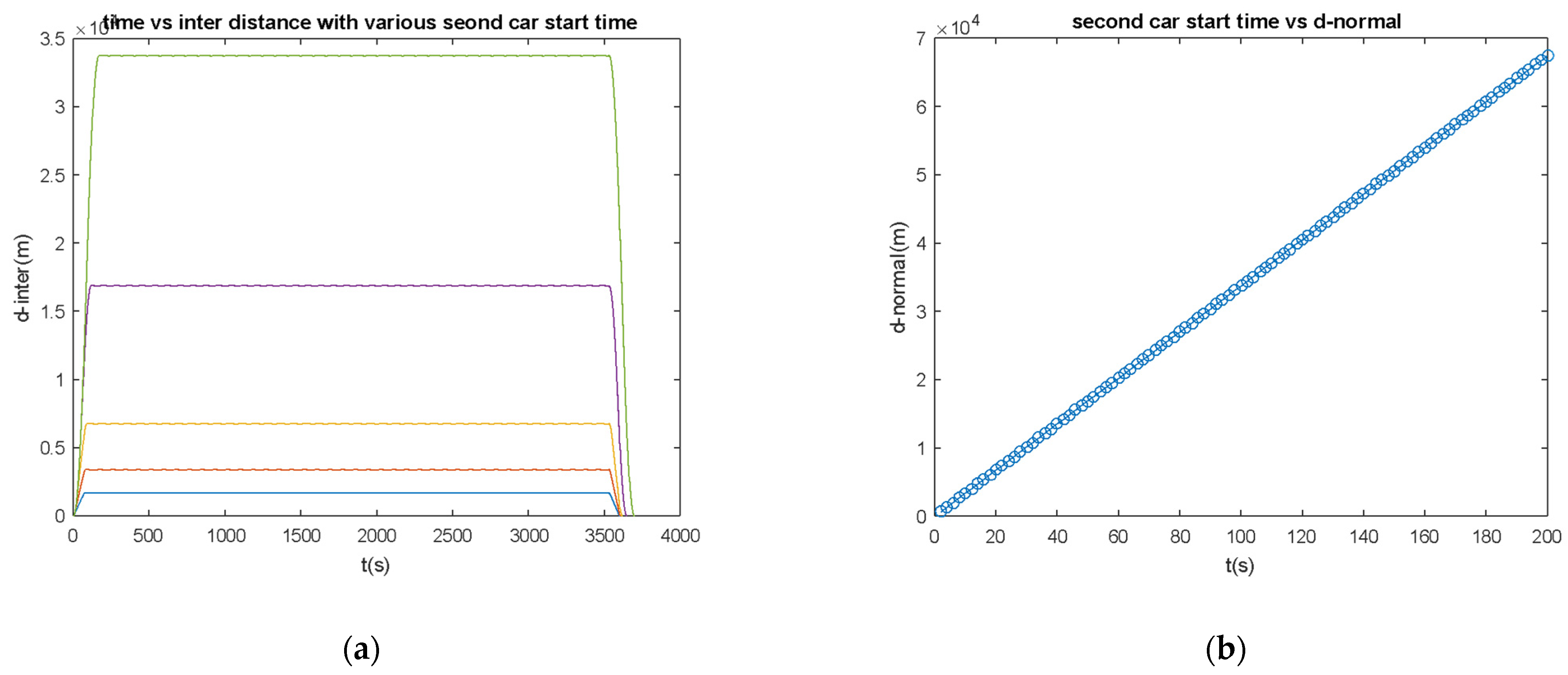
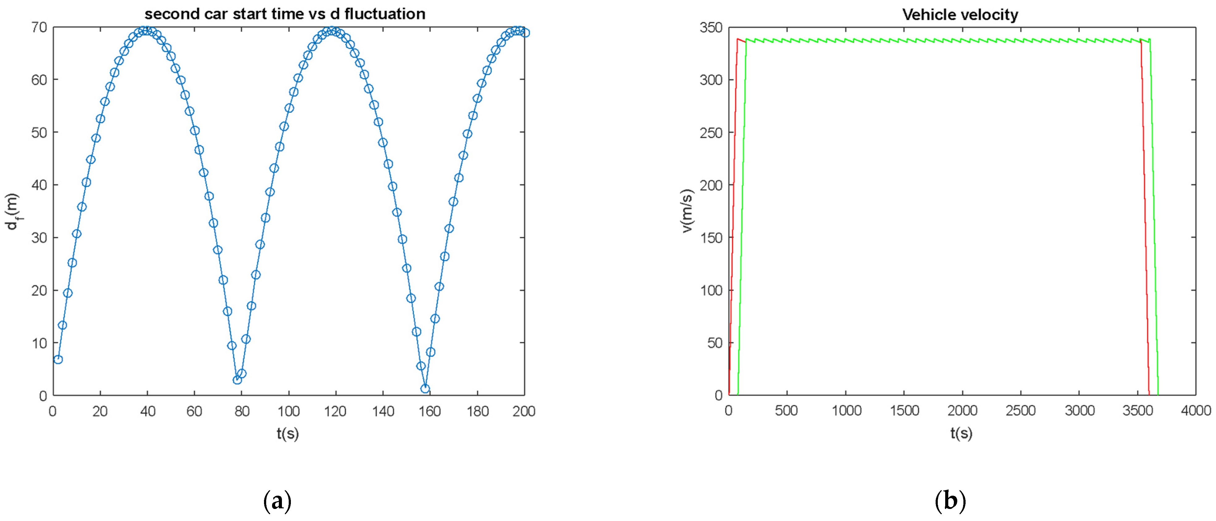
5.2. Second Vehicle Start Time Actuation and Characteristics

After studying the velocity error effect, we find out, when the error is smaller, the inter-distance fluctuation is smaller. Now we fix the error at 1% and vary the second vehicle start time. Figure 12a shows the inter-distance with various second vehicle start time at 5 [s], 10 [s], 20 [s], 50 [s], 100 [s]. Inter-distance fluctuation normal value(d_normal), which refers to the average of maximum value and minimum value of fluctuation region, is increasing when the second vehicle start time increases, see Figure 12b. The nodes number is kept the same when the error increases, which means the nodes number is the only function of error. Moreover, the pushing time is also kept the same when error increases, which means the pushing time is also only a function of error.

Interestingly, the inter-distance fluctuation is showing a periodical pattern when error increases, shown in Figure 13a. From the figure, we can see, at a certain point, the fluctuation can be maximum, and at a certain point, the fluctuation can be zero, which means, at some second vehicle start time, there is no fluctuation for inter-distance. If we take the first zero fluctuation point, which is 76.64 [s], the velocity simulation is shown in Figure 13b, we can see that the two vehicles’ velocity figures become overlapped after the first vehicle’s velocity drops down to a minimum. Then the first pushing region of the first vehicle coincides with the second vehicle acceleration. Moreover, the corresponding inter-distance is shown in Figure 14a. After the inter-distance reaches to maximum, then the inter-distance is keeping the same value, there is no fluctuation anymore.

The second vehicle start period for zero inter-distance fluctuation is a push-down cycle time. Figure 14b shows the cycle time for different velocity errors. For specific velocity error rates, when the second car starts at an integral number of cycle times, the inter-distance fluctuation can always be minimized.

6. Conclusions

In this paper, operational control of high-speed capsular vehicles, numerical analysis, and evaluation has been performed with multiple control parameters. The goal is to find the best scenario to minimize the inter-distance and its fluctuation. The major accomplishment of this effort is that we generated a dynamic motion model for our unique system and proceeded with a numerical analysis toward operational control of high-speed vehicles. After we studied the numerical analysis of the system, we found out:

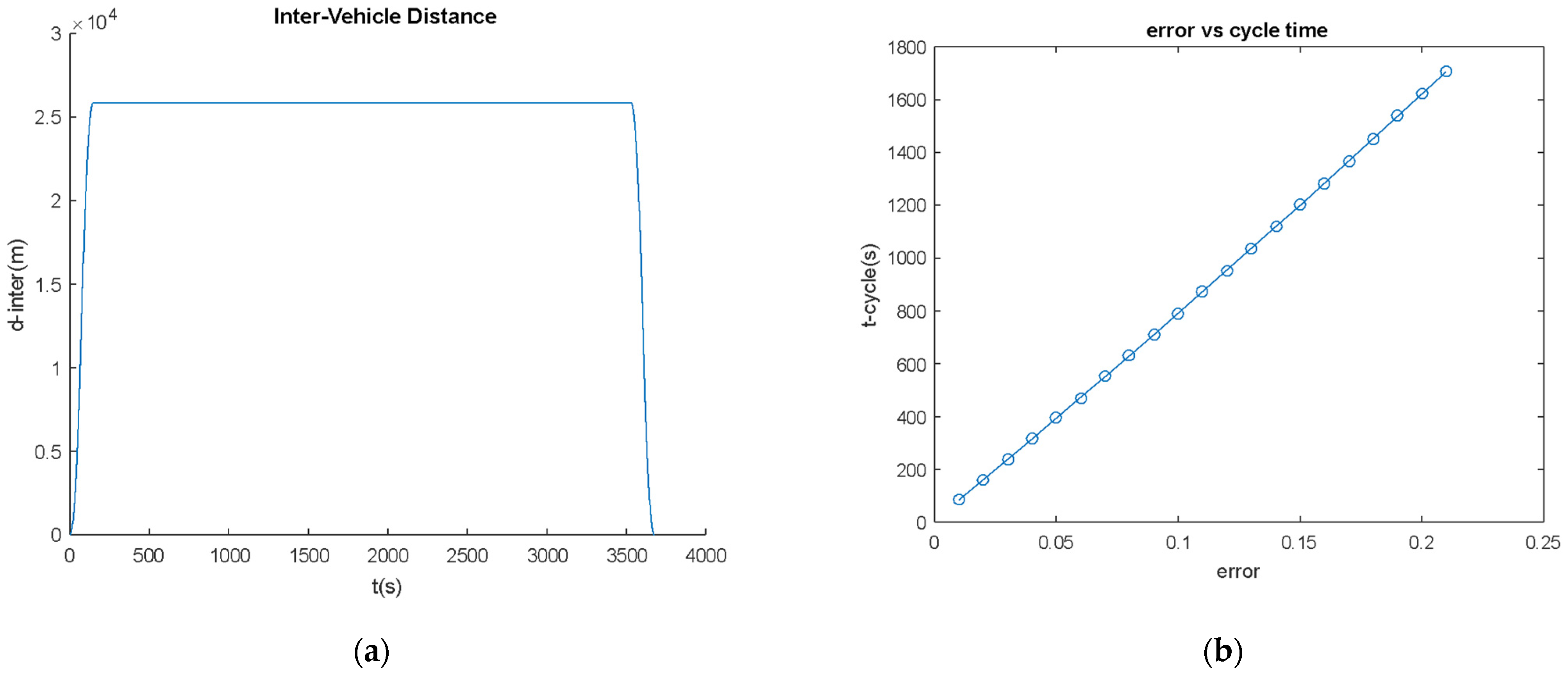
• Inter-distance is a function of error rate and second car start time, the magnitude range is determined by second car start time.
• Inter-distance fluctuation rate is a function of error rate and second car start time. However, it can be minimized by choosing the correct second car start time.
• If the second car start time is chosen as an integer number of push-down cycle times at a specific velocity error rate, the inter-distance fluctuation can be zero.

Through this important finding based on the numerical evaluation, authors can conclude that we can design a control law to minimize the inter-distance and fluctuation rate by setting error rate and second car start time aiming for maximized passenger or freight rate with given time for future application.

References

1. Xiangming, W. Experience in operation and maintenance of Shanghai Maglev demonstration line and further application of Maglev in China. In Proceedings of the Maglev’ 2006 Germany Proceedings, Dresden, Germany, 13–15 September 2006; Volume 1, pp. 17–19. [Google Scholar]
2. Leheis, S. High-speed train planning in France: Lessons from the Mediterranean TGV-line. Transp. Policy 2012, 21, 37–44. [Google Scholar] [CrossRef] [Green Version]
3. Hood, C. Shinkansen: From Bullet Train to Symbol of Modern Japan; Routledge: London, UK, 2006. [Google Scholar]
4. Sunduck, D.; Keun-Yul, Y.A.N.G.; Jae-Hoon, L.E.E.; Byung-Min, A.H.N. Effects of Korean Train Express (KTX) operation on the national transport system. Proc. East. Asia Soc. Transp. Stud. 2005, 5, 175–189. [Google Scholar]
5. Song, D.; Yang, C.H.; Hong, S.K.; Kim, S.B.; Woo, M.S.; Sung, T.H. Study on application of piezoelectricity to Korea Train eXpress (KTX). Ferroelectrics 2013, 449, 11–23. [Google Scholar] [CrossRef]
6. Abdelrahman, A.S.; Sayeed, J.; Youssef, M.Z. Hyperloop Transportation System: Analysis, Design, Control, and Implementation. IEEE Trans. Ind. Electron. 2017, 65, 7427–7436. [Google Scholar] [CrossRef]
7. Nar, P.; Narkar, B.; Subhash, S.; Palekar, L.S.; Ramchandra, Y. Review of Hyperloop Technology: A New Mode of Transportation. Int. J. Sci. Res. Dev. 2018, 6, 73–75. [Google Scholar]
8. Nemchenko, A.; Boyarskaya, A. The Hyperloop High-Speed Train. 2017. Available online: https://rep.bntu.by/bitstream/handle/data/33629/The%20Hyperloop%20High-Speed%20Train.pdf?sequence=1 (accessed on 2 May 2019).
9. Ross, P.E. Hyperloop: No Pressure. IEEE Spectr. 2015, 53, 51–54. [Google Scholar] [CrossRef]
10. Singh, A.; Mahajan, A.; Mahajan, N.; Gaikwad, A. Hyperloop Transportation System. Int. Res. J. Eng. Technol. 2019, 6, 2554–2558. [Google Scholar]
11. Dhandapani, C. A Review: Hyperloop Transportation System. Cikitusi J. Multidiscip. Res. 2019, 6, 5. [Google Scholar]
12. Janzen, R. Transpod ultra-high-speed tube transportation: Dynamics of vehicles and infrastructure. Procedia Eng. 2017, 199, 8–17. [Google Scholar] [CrossRef]
13. Ji, W.Y.; Jeong, G.; Park, C.B.; Jo, I.H.; Lee, H.W. A study of non-symmetric double-sided linear induction motor for Hyperloop All-In-One System (propulsion, levitation, and guidance). IEEE Trans. Magn. 2018, 54, 1–4. [Google Scholar] [CrossRef]
14. Lluesma-Rodríguez, F.; González, T.; Hoyas, S. CFD simulation of a hyperloop capsule inside a closed environment. Results Eng. 2021, 9, 100196. [Google Scholar] [CrossRef]
15. Oh, J.S.; Kang, T.; Ham, S.; Lee, K.S.; Jang, Y.J.; Ryou, H.S.; Ryu, J. Numerical analysis of aerodynamic characteristics of hyperloop system. Energies 2019, 12, 518. [Google Scholar] [CrossRef] [Green Version]
16. Yang, Y.; Wang, H.; Benedict, M.; Coleman, D. Aerodynamic simulation of high-speed capsule in the Hyperloop system. In Proceedings of the 35th AIAA Applied Aerodynamics Conference, Denver, CO, USA, 5–9 June 2017. [Google Scholar]
17. Opgenoord, M.M.J.; Merian, C.; Mayo, J.; Kirschen, P.; O’Rourke, C.; Izatt, G. MIT Hyperloop Final Report; Massachusetts Institute of Technology: Cambridge, MA, USA, 2017. [Google Scholar]
18. Dudnikov, E. Advantages of a new Hyperloop transport technology. In Proceedings of the 2017 Tenth International Conference Management of Large-Scale System Development (MLSD), Moscow, Russia, 2–4 October 2017. [Google Scholar]
19. Almujibah, H.; Kaduk, S.I.; Preston, J. Hyperloop—Prediction of Social and Physiological Costs. Transp. Syst. Technol. 2020, 6, 43–59. [Google Scholar] [CrossRef]
20. Zhang, J.; Liu, L.; Han, B.; Li, Z.; Zhou, T.; Wang, K.; Wang, D.; Ai, B. Concepts on Train-to-Ground Wireless Communication System for Hyperloop: Channel, Network Architecture, and Resource Management. Energies 2020, 13, 4309. [Google Scholar] [CrossRef]
21. Zhang, J.; Liu, L.; Wang, K.; Han, B.; Piao, Z.; Wang, D. Analysis of the Effective Scatters for Hyperloop Wireless Communications Using the Geometry-Based Model. In International Conference on Machine Learning for Cyber Security; Springer: Berlin/Heidelberg, Germany, 2020. [Google Scholar]
22. Nikolaev, R.; Idiatuallin, R.; Nikolaeva, D. Software system in Hyperloop pod. Procedia Comput. Sci. 2018, 126, 878–890. [Google Scholar] [CrossRef]
23. Van Goeverden, K.; Milakis, D.; Janic, M.; Konings, R. Analysis and modelling of performances of the HL (Hyperloop) transport system. Eur. Transp. Res. Rev. 2018, 10, 41. [Google Scholar] [CrossRef]
24. Lafoz, M.; Navarro, G.; Torres, J.; Santiago, Á.; Nájera, J.; Santos-Herran, M.; Blanco, M. Power supply solution for ultrahigh speed hyperloop trains. Smart Cities 2020, 3, 642–656. [Google Scholar] [CrossRef]
25. Janić, M. Estimation of direct energy consumption and CO2 emission by high speed rail, transrapid maglev and hyperloop passenger transport systems. Int. J. Sustain. Transp. 2021, 15, 696–717. [Google Scholar] [CrossRef]
26. Ahmadi, E.; Alexander, N.A.; Kashani, M.M. Lateral dynamic bridge deck–pier interaction for ultra-high-speed Hyperloop train loading. In Proceedings of the Institution of Civil Engineers-Bridge Engineering; Thomas Telford Ltd.: London, UK, 2020; Volume 13, pp. 198–206. [Google Scholar]
27. Bose, A.; Viswanathan, V.K. Mitigating the Piston Effect in High-Speed Hyperloop Transportation: A Study on the Use of Aerofoils. Energies 2021, 14, 464. [Google Scholar] [CrossRef]
28. Eichelberger, M.; Geiter, D.T.; Schmid, R.; Wattenhofer, R. High-Throughput and Low-Latency Hyperloop. In Proceedings of the 2020 IEEE 23rd International Conference on Intelligent Transportation Systems (ITSC), Rhodes, Greece, 20–23 September 2020. [Google Scholar]
29. Sarin, M.; Overton, M. Complex Hyperloop Capsule Safety Requirements and Risk Mitigations. In Proceedings of the 36th International System Safety Conference, Phoenix, AZ, USA, 13–17 August 2018. [Google Scholar]
30. Hyde, D.J.; Barr, L.C.; Taylor, C. Hyperloop Commercial Feasibility Analysis: High Level Overview; John, A., Ed.; Volpe National Transportation Systems Center (US): Cambridge, MA, USA, 2016.
31. Alexander, N.A.; Kashani, M.M. Exploring Bridge Dynamics for Ultra-High-Speed, Hyperloop, Trains. Structures 2018, 14, 69–74. [Google Scholar]
32. Mitropoulos, L.; Kortsari, A.; Koliatos, A.; Ayfantopoulou, G. The Hyperloop System and Stakeholders: A Review and Future Directions. Sustainability 2021, 13, 8430. [Google Scholar] [CrossRef]
33. Gkoumas, K. Hyperloop Academic Research: A Systematic Review and a Taxonomy of Issues. Appl. Sci. 2021, 11, 5951. [Google Scholar] [CrossRef]
Figure 1. An exemplary picture of high-speed connected vehicles (image courtesy by China Railway High-speed).
Vehicles 04 00002 g001
Figure 2. Conceptual rendering of capsular vehicles (image from KRRI).
Vehicles 04 00002 g002
Figure 3. EDS force simulation with velocity.
Vehicles 04 00002 g003
Figure 4. (a) Input force and (b) vehicle accleration output when (m1 = 24,000 [kg] (blue), m2 = 26,000 [kg] (red), t_scndstart = 50 [s]) in the duration of 3600 [s] of operation, (red) and (green) respectively.
Vehicles 04 00002 g004
Figure 5. (a) Acceleration response in the initial stage (before the velocity reaches 19.82 [m/s] or initial 120 [s] (red and then green), and (b) while the vehicle is cruising when (m1 = 24,000 [kg] (red), m2 = 26,000 [kg] (green), t_scndstart = 50 [s]).
Vehicles 04 00002 g005
Figure 6. (a) Acceleration output in the final state near 3600 [s] when (m1 = 24,000 [kg] (red), m2 = 26,000 [kg] (green), t_v2 = 50 [s]) and (b) velocity response corresponding to the acceleration output Figure 4b and input force as shown in Figure 4a.
Vehicles 04 00002 g006
Figure 7. (a) Each vehicle’s displacement (m1 = 24,000 [kg] (red), m2 = 26,000 [kg] (green), t_scndstart = 50 [s]), and (b) inter-distance between two vehicles when when (m1 = 24,000 [kg], m2 = 26,000 [kg], t_scndstart = 50 [s]) in the duration of 3600 [s] of operation (blue).
Vehicles 04 00002 g007
Figure 8. (a) Regulated velocity response with error = 0.1 rate (red for 24,000 [kg], green for 26,000 [kg], and (b) Corresponding force input to generate the regulated velocity as shown in Figure 8a when (m1,m2) = (24,000 (blue),26,000 (red) [kg], t_scnd = 50 [s]) respectively.
Vehicles 04 00002 g008
Figure 9. (a) Acceleration output when regulated velocity with error = 0.1 rate, (red for 24,000 [kg], green for 26,000 [kg], and (b) Vehicles’ displancement when regulated velocity with error = 0.1 rate (m1,m2) = (24,000, 26,000 [kg], t_scnd = 50 [s]) respectively.
Vehicles 04 00002 g009
Figure 10. (a) Inter-distance between two vehicles when regulated velocity with error = 0.1, and (b) Inter-distnace with various error rates (error = 1%, 2%, 5%, 10%, 20%, t_scndstart = 50 [s], m1 = 24,000 [kg], m2 = 26,000 [kg]), green, purple, yellow, orange, blue respectively.
Vehicles 04 00002 g010
Figure 11. (a) Various error rates vs. number of nodes, and (b) various error rates vs. pushing time when (error = 1%, 2%, 3%, …, 20%, t_scndstart = 50 [s], m1 = 24,000 [kg], m2 = 26,000 [kg]).
Vehicles 04 00002 g011
Figure 12. (a) Inter-distance with various second vehicle start time and (b) second car’s start time vs. inter-distance flunctuation normal distance when (error = 1%, t_scndstart = 5, 10, 20, 50, 100 s, m1 = 24,000 [kg], m2 = 26,000 [kg]) green, purple, yellow, orange, blue respectively.
Vehicles 04 00002 g012
Figure 13. (a) Inter-distance fluctuation with various second vehicle start time, and (b) velocity response (error = 1%, t_scndstart = 5 [s], 6 [s], 7 [s], …, 100 [s], m1 = 24,000 [kg] (red), m2 = 26,000 [kg] (green)).
Vehicles 04 00002 g013
Figure 14. (a) Inter-distance at error = 1%, t_scndstart = 76.64 [s], and (b) various error rates vs. push-down cycle time when (m1 = 24,000 [kg], m2 = 26,000 [kg]).
Vehicles 04 00002 g014