Article

Effectiveness of Climbing Lanes for Slow-Moving Vehicles When Riding Uphill: A Microsimulation Study

1
Department of Civil, Constructional and Environmental Engineering, University of Rome La Sapienza, Via Eudossiana 18, 00184 Rome, Italy
2
Civil Engineer, 00100 Rome, Italy
*
Author to whom correspondence should be addressed.
Vehicles 2023, 5(3), 744-760; https://doi.org/10.3390/vehicles5030041
Submission received: 22 May 2023 / Revised: 25 June 2023 / Accepted: 26 June 2023 / Published: 28 June 2023

Abstract

:
Long uphill stretches of single-carriageway rural roads with one lane per travel direction may reduce the Level of Service (LoS), due to the decreased speed of heavy vehicles. In those circumstances, a slowdown of traffic, resulting in the formation of platoons, may be generated due to the difficulty of performing overtaking maneuvers safely. To solve this critical issue, an additional (climbing) lane for slow vehicles may be included in the road platform. This study aims to evaluate the effectiveness of such climbing lanes in a real case in Italy (National Road n. 4 “Via Salaria”—around 44+000 km). Using a microsimulation model implemented in VISSIM, the study analyzes speeds and travel times, delays, and queuing waiting times, comparing the Actual Scenario (AS) without climbing lanes, with two counterfactual scenarios: the first one (CS1) with three stretches of climbing lanes, and the second one (CS2), with just two stretches, in which the first two additional lanes of CS1 are merged together. The obtained results confirm the effectiveness of installing climbing lanes on road sections with the described characteristics, and the potential of microsimulation models also to carry out such kind of evaluations.

1. Introduction

Single-carriageway rural roads with just one lane per each travel direction have safety- and functionality-related issues in steep longitudinal slopes stretches [1,2]. Different vehicles with different performance properties, depending on their power-to-weight ratio, result in various speeds along uphill grades. Both passenger cars and heavy vehicles have been extensively analyzed with regard to their characteristics interactions with road infrastructures and users [3,4]. In particular, the AASHTO 2018 “A Policy on Geometric Design of Highways and Streets” [5] presents vehicle operating characteristics on grades, and establishes relationships between grades and their lengths with operating speed.
Generally, the presence of heavy vehicles and the difficulty of performing overtaking maneuvers cause “platoons” to form, generating delays in travel times and a lowering of the Level of Service, LoS. The “Geometric Design of Highways and Streets” [5] provides a series of performance diagrams for heavy vehicles, according to different power-to-weight ratio, to evaluate their speed changes in covering variable slope sections [6,7], both in acceleration and deceleration. Excessively low speed values of heavy-vehicles compared to average operating speeds can generate passenger cars queuing, increasing travel times, and becoming a possible incentive for improper and potentially dangerous overtaking [8]. The operating condition decay results in a road LoS drop, which is possible to define on the basis of two indicators, according to the HCM [9]:
-
Percent time-spent-following (PTSF): average percentage of travel time that vehicles spend queuing behind heavy and slow vehicles, unable to overtake;
-
Average travel speed (ATS): ratio between road section length and both direction vehicles travel time, during a set time interval.
To ensure an adequate operating level even in possible traffic slowdowns due to the presence of heavy vehicles on long stretches of uphill road, a separate climbing lane for slow-moving vehicles can be added to the existing platform. Its use is justified [5,9] when:
-
Upgrade traffic flow rate is in excess of 200 veh/h;
-
Upgrade truck flow rate is in excess of 20 veh/h;
-
A 15-km/h or greater speed reduction is expected for a typical heavy truck, or level of service E or F exists on the grade, characterized by unstable or breakdown flows, or a reduction of two or more levels of service is experienced when moving from the approach segment to the grade.
In Italy, the Ministerial Decree of 5 November 2001 [9] states that the introduction of supplementary lanes is necessary when traffic conditions may become critical. This can be ascertained by considering:
-
The slowdown suffered by heavy vehicles on uphill stretches, to be considered intolerable if the speed of such vehicles is reduced to less than 50% of that of passenger cars on the same stretch;
-
The decay in traffic quality and safety conditions in relation to the percentage of heavy vehicles and the expected traffic volume.
Several studies have researched and demonstrated the functionality and influence of climbing lanes on road capacity and safety by implementing microsimulation models. Microsimulation allows the reconstruction of traffic evolution in a road network and the interaction between vehicles in terms of overtaking, lane changes, and queuing [10,11]. Yeo et al. [12] evaluated the operational efficiency and safety resulting from an auxiliary lane using the OFFA microsimulation software; the analysis was conducted by evaluating the total delay time and driving speed. The simulation showed that benefits to the functionality of the analyzed section exist if the traffic volumes do not exceed 900 veh/h and the percentage of heavy traffic is around 30–40%. Ko et al. [13] analyzed the dynamic management of climbing lanes on a highway sections using the VISSIM microsimulation software. The study proposed to open the climbing lane when the average speed on the main lane falls below 80 km/h, and to close it when the desired operating conditions are restored. The results showed an increase in the average speeds by up to 15.6%, a reduction in average delay times by 30.6%, and a reduction in the number of merging conflicts by up to 62.1%. Other studies investigated traffic flow characteristics and road safety enhancement through the VISSIM software, thanks to the addition of a climbing lane [14,15]. The results showed highest speeds and a reduction in head-on collisions between the two opposing vehicular streams. Valencia-Alaix et al. [16] conducted a study on uphill gradients of a two-lane road, one in each direction, using the TWOPAS microsimulation software. The analysis was carried out by considering different scenarios in which a climbing lane would be included, varying the values of longitudinal slope, vehicular flow, and percentage of heavy vehicles. The operational efficiency of the climbing lane was studied in terms of PTSF and the ATS. An increase in PTSF between 9 and 22% has been observed, while ATS had improved as the number of heavy vehicles has increased. Hou et al. [17] conducted a statistical analysis according to the Propensity Score Matching method to quantify the effect of including climbing lanes on a freeway segment. A comparison of the scenarios with and without the additional lanes demonstrated in the first case a reduction in the number of accidents, in the accidents per kilometer, and in the accidents per 100 million vehicle/traveled kilometers by 18.3%, 17.5%, and 17.4%, respectively.
In this paper, in accordance with the scientific literature, we aim to develop a preventive analysis to evaluate the effectiveness of several alternative configurations proposed to solve critical issues on an existent road section (National Road n. 4 “Via Salaria”). Traffic microsimulation models, in fact, correctly calibrated and validated [18,19], attempt to simulate drivers’ behavior within a predefined road network. They can predict the likely impact of changes in driving behaviors and choices resulting from changes to the infrastructure itself or to vehicular flows or types. For this reason, to analyze the possible effects that the addition of one or more climbing lanes might generate on the road network, it was decided to exploit this ability of the models. In particular, the case study was examined using a microsimulation model implemented in the VISSIM software. The investigation was carried out on an approximately 5-km length stretch of the road, starting at 44+000 km, which is characterized by steep gradients.
The paper is composed of three parts, and the content of each is as follows: (1) case study input data description and microsimulation analyses through a calibrated and validated model, (2) results coming from a comparison of speed and travel times, delays, and queuing waiting times between the actual scenario (AS), without climbing lanes, and two counterfactual scenarios (CS1 and CS2) marked by the presence of the auxiliary lanes, and (3) experimental verification which confirms the effectiveness of climbing lanes in both functional and safety terms on rural roads with one lane in each travel direction.

2. Materials and Methods

This paper proposes a comparative analysis of the benefits deriving from climbing lanes along a section of a single-carriageway rural road with one lane in each direction. The methodology is divided into two macro phases: the first one involves the identification of the case study and the geometric and traffic data necessary to define the operating conditions, while the second phase implements the simulation of the analyzed scenarios after a calibration and a validation of the adopted software.

2.1. Case Study

2.1.1. Road Geometrical and Functional Features

Important upgrading works are planned for the National Road n. 4 Via Salaria aimed at improving its operating conditions. In particular, in the actual scenario, AS, between progressive 42+800 km and 49+000 km, there is a succession of slopes which results in disruption to traffic and safety issues for the infrastructure. The developed model aims at simulating the traffic conditions of Via Salaria in the road section considered (Figure 1).
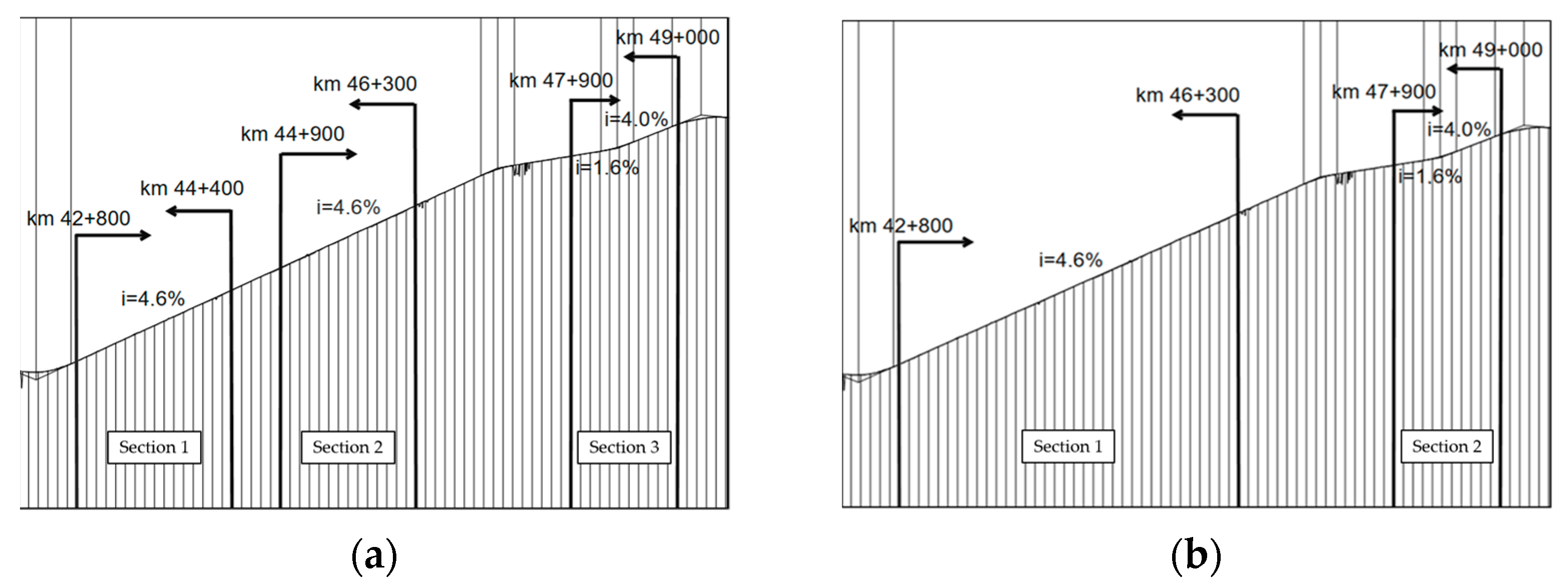
Several design solutions have been proposed for the functional upgrading and enhancement of the road; among them, there is one project, CS1, which includes three sections of climbing lane (Figure 2a), where the speed of heavy vehicles falls below the 50% of the speed of passenger cars, in accordance with DM 2001 [20]:
(1)
The first one in the section between 42+800 km e and 44+400 km;
(2)
The second one in the section between 44+900 km and 46+300 km;
(3)
The last one in the section between 47+900 km and 49+000 km.
An alternative scenario, CS2, has been studied, which involves just 2 sections of climbing lane, between 42+800 km and 46+300 km, and from 47+900 km to 49+000 km, to comply with a spacing of not less than 600 m between additional lanes, as stated in the Italian guideline [20] (Figure 2b).
The geometry of the road has been reconstructed from the plano-altimetric information made available by the road Administration owner of the examined road [21]. Within the VISSIM simulation software, the layout configuration was represented through a series of nodes and arcs (Links e Connectors), while the elevation trend was defined by assigning all links their own longitudinal slope values. Finally, the cross-section dimensions of the secondary rural road platform have been associated, according to the classification of the Italian guideline [20].

2.1.2. Traffic Data Analysis—LoS Calculation

The traffic data collection is a necessary step to enable the functional condition of the examined road section to be correctly defined, and to stabilize the percentage of heavy vehicles out of the entire traffic flow. The traffic data used to develop the present study are those collected by the Automatic Statistical Traffic Detection System of the Italian national road network manager, ANAS SpA [22]. The Traffic Observatory is a structure that the company mainly uses to provide traffic data and information to users; all the sensors send their data to a central Platform for Monitoring and Analysis—called PANAMA—and the reliability of the acquired data is ensured by a series of control procedures [23]. For the case study analyzed, Anas stations 64 and 2350, located at 36+000 km and 58+000 km of Via Salaria, respectively, were identified because they are the two point-based sensors closest to the road section under investigation (Figure 3). The dataset for 5 months of fall-winter days is aggregated every 5 min and divided by travel direction: A (ascending flow directed towards Rieti) and D (descending flow direct towards Rome).
The peak hour traffic flows have been averaged among the two stations recordings, and are summarized in Table 1, divided by the two travel directions, in the morning and in the afternoon, and between weekdays and weekends, as follows:
Among the various information provided with the traffic data is the classification of the vehicles according to the “Famas 9+1” classification scheme, which divides the traffic into nine vehicular categories, plus one that is none of the above ones: Motorcycles, Cars, Car Trailers, Vans, Trucks < 7.5 m, Trucks > 7.5 m, Articulated trucks, Road trains, Buses, and Others. Table 2 shows the vehicular sub-categories in the two travel directions:
The LoS of the examined section has been assessed according to the HCM [9], through the definition of the ATS and PTSF. The performed calculation showed a “C” LoS, characterized by a stable flow, at or near free flow conditions, with reference to the data from the two stations in the most critical month and hour (between 5 p.m. and 6 p.m.).

2.2. Microsimulation

Traffic simulation is a widely applied method in scientific research on modeling, planning and development of traffic networks and systems [24,25]. The aim is to accurately recreate observed and measured traffic on the road. In particular, three simulation models can be distinguished, classified according to their area of application: microscopic, macroscopic and mesoscopic modeling [26].
In this paper, the investigation was performed through the VISSIM software, produced by the German company PTV [27]. It is a discrete, randomized, microscopic simulation software that assumes a time step of 1/10th of a second. VISSIM provides an interface to visualize vehicle motion with 2D or 3D animation and to analyze various traffic conditions by varying lane configuration, traffic composition, traffic signals, bus stops, etc. [28,29]. The software has a four-level structure: traffic supply, traffic demand, traffic control facilities, and data output [28]. The first part describes the physical infrastructure, while the second part indicates the demand of people and vehicles running on the physical infrastructure. The third level indicates the traffic control facilities (i.e., priority rules between primary and secondary roads, and traffic lights). Finally, output data include dynamic demonstration and traffic control status, statistical data, and vehicle status.
The microscopic modeling method has been adopted for the present study, based on the sub-models of car-following, lane-changing, and gap acceptance [24]. It has been necessary to perform a calibration and validation of the studied model [30], before the implementation of the analyzed scenarios.

2.2.1. Calibration Phase

Calibration is a necessary step because no model can return complete accuracy in reproducing all possible traffic conditions. Every microsimulation software has within it a set of user-adjustable parameters for the purpose of calibrating the model by adapting it to local conditions. The goal of calibration is, therefore, to find the set of parameter values that can best reproduce the observed reality. There are two levels of parameter setting for calibration, a global and a local one [31]. From the global perspective, basic settings regarding simulation, traffic, and vehicular fleet characteristics are considered. In Table 3, the default values and those adopted for the model definition are shown:
Regarding the local level, the parameters characterizing the car-following and lane-changing sub-models are considered. In the examined case study, for the car-following and lane-changing sub-models, the default parameters (Table 4 and Table 5) provided by the software have been applied and subsequently validate:
As stated before, and according to the scientific literature [32,33], the variables of a microscopic traffic model can be calibrated in respect of two different levels of investigation: a macroscopic or global level, e.g., traffic volumes and speeds’ distributions’ variables, and a microscopic or local level, e.g., car following or lane changing parameters. In the present study, just the global level has been calibrated, as shown in Table 3, while the local level has kept the default parameters unchanged (Table 4 and Table 5).

2.2.2. Validation Phase

Model validation is the step following the calibration one and is the process through which it is verified whether the simulated model can correctly reproduce real traffic conditions [34]. In this study, since the default parameters of the software were used for the local level, we have verified whether the basic settings actually offer the possibility of faithfully reproducing real traffic conditions through microsimulation. As stated in Section 2.1.2, the available traffic characteristic are speeds and hourly volumes.
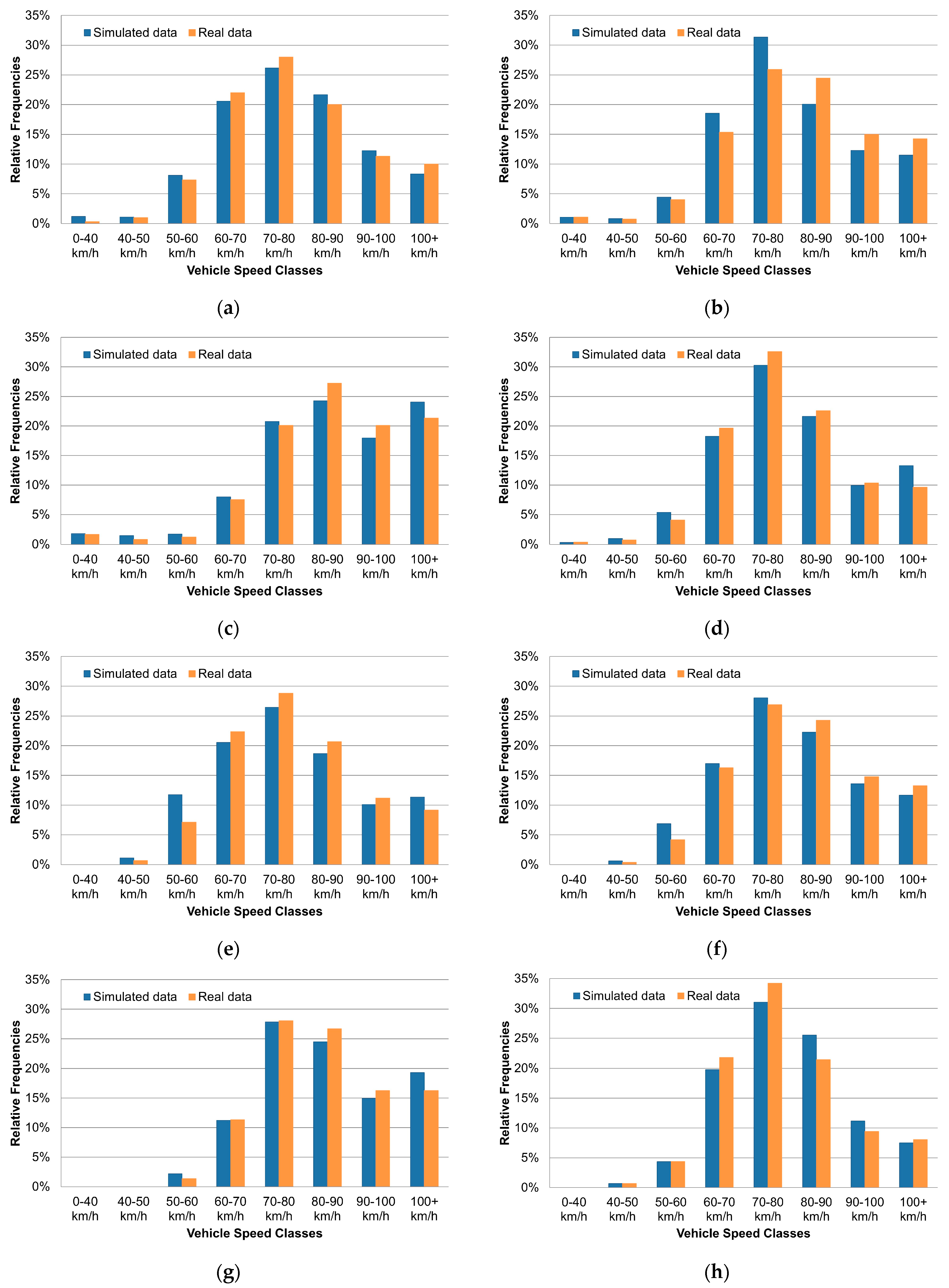
From the actual data, it has been possible to obtain frequency histograms (Figure 4a–h), useful for validating the model in terms of speed class distributions, and cumulative distribution curves of travel operating speeds measured by the sensors. VISSIM enables to create desired speed curves for each individual vehicular category: starting from the actual operating speeds, the desired speeds in free-flow conditions have been hypothesized.
As it can be seen from the histograms in Figure 4, the results obtained dividing the sample into speed classes show an acceptable level of actual data reproducibility by the software-simulated model. Moreover, a chi-square ( χ 2 ) goodness of fit test has been applied to understand how well the microsimulation model fits the set of observations. The results obtained are presented in Table 6:
With a 7 degrees of freedom (8 speed classes) and a significance level (α) equal to 0.05, we have compared the results with a tabled chi-square critical value equal to 14.067. Since the χ 2 values are less than the critical value, then the differences between the observed and simulated distributions are not statistically significant. The fit between the distributions is good enough: only 5% of the data are greater than 14.067.

2.2.3. Actual Microsimulation Analyses

To simulate the different traffic scenarios with the micro-simulation software Vissim, 100 simulations were performed for each case stady, each lasting 3600 s. The parameters with which the performance of each vehicle category has been evaluated are the following:
-
Speed;
-
Travel times and delay times;
-
Queue waiting times to determine the travel speeds of the vehicles, data collection points—the so-called control points—have been added to relevant sections, such as the starting and ending points of the analyzed road trunk, and the starting and ending points of the three climbing lanes. Through the control points the evaluation of travel times and delays and, consequently, queue waiting times have been also performed.

3. Results and Discussion

The evaluation of the effectiveness of climbing lanes has been conducted on an around 5 km long road segment of the National Road n. 4 Via Salaria, characterized by steep gradients. Different traffic scenarios were simulated with the VISSIM microsimulation software, and 100 simulations were performed for each scenario analyzed, each lasting 3600 s. The VISSIM software considers the stochastic nature of road traffic by implementing automotive models with parameters that use stochastic distributions. According to Table 2, the software defines vehicle groups with similar technical characteristics and physical driving behavior, but the dynamic parameters of vehicles belonging to a same group assume different values extracted from a stochastic distribution of the same. For example, VISSIM does not adopt a single acceleration and deceleration value but uses functions to represent the variability associated with driver behavior. In addition, VISSIM applies weight and power distributions only for the types of vehicles in the HGV category. The program calculates the power-to-weight ratio in kW/t, which can take values between 7 and 30 kW/t. Depending on the ratio obtained, an acceleration/deceleration curve is associated to the vehicle accordingly [29]. To ensure slow moving vehicles just on the climbing lanes, the option “Blocked-Vehicles: Car” was set directly to the link corresponding to the additional lane. The investigation is based on the comparison between the actual scenario (AS) and two alternative scenarios (CS1 and CS2) in terms of:
-
Vehicle speeds;
-
Travel times and delay times;
-
Queuing waiting times.
The 100 simulations values obtained in each studied scenario have been measured at the nodes, at the beginning and end sections of the investigated segment and at the beginning and end sections of the climbing lanes, and then averaged.

3.1. Vehicle Speeds

The study focused on the determination of the average speeds for each vehicular category (Cars, Buses, and HGV) along the examined segment, in the three analyzed scenarios, AS, CS1, and CS2 (Figure 5):
Figure 5a compares the average speeds’ trends of light vehicles in the three analyzed scenarios: it is observed that in general, average speeds decrease progressively along the segment, due to the presence of high longitudinal uphill gradients. In detail, the comparison shows that in AS, compared to the CS1 and CS2 scenarios, the average speeds are significantly reduced because of the interference between heavy and light vehicles. Heavy vehicles, in fact, in lack of additional lanes for uphill travel, limit the driving of cars. Comparing the different vehicular categories’ speeds in the stretch of road between 42+800 km and 46+300 km, characterized by a longitudinal gradient of 4.6%, in the AS, light vehicles travel at sharply reduced speeds, influenced by bus and HGV speeds ranging between 50 and 60 km/h (Figure 5a–c). In the section, between 47+200 km and 48+300 km, the longitudinal slope decreases to 1.6% and there is an increase in the average speeds. In general, there is a marked improvement in vehicular performances in CS1 and CS2 scenarios compared to AS: vehicles manage to maintain their average speed around the desired speed along the entire route. Passenger cars and HGVs show that the CS2 is the best solution in terms of average speeds along the entire route, whereas the buses’ average speeds are not markedly different between the two counterfactual scenarios. The greatest speed difference of about 4 km/h, in fact, is localized in a short section, while in the rest of the studied trunk the average speeds are almost identical. This is due to the stochastic nature of a microsimulation model.
Frequency histograms by speed classes for light vehicles have been realized to assess the disturbance of heavy vehicles (“HGVs” and Buses”) in sections with higher longitudinal gradient. Figure 6 shows the histograms at 42+800 km and 49+000 km:
At the beginning of the track, see Figure 6a, the frequency distribution of light vehicle speeds shows a normal-type pattern around the mean value in all the three scenarios. As the distances increase to the final section (Figure 6b), an increasing number of light vehicles are observed in the AS moving at low speeds, due to the disturbance caused by heavy vehicles, which contribute to the phenomenon of “platooning” that generates functionality and safety problems. In the other 2 scenarios, CS1 and CS2, however, there is generally a higher frequency of higher speed classes.

3.2. Travel Times and Delay Times

VISSIM can estimate the average travel time of specific routes if they are defined in the network. Each route consists of a departure section and a destination section. The average travel time of a vehicle (including waiting or stopping time) is defined as the time between the instant of crossing the first cross-section and the instant of crossing the second cross-section.
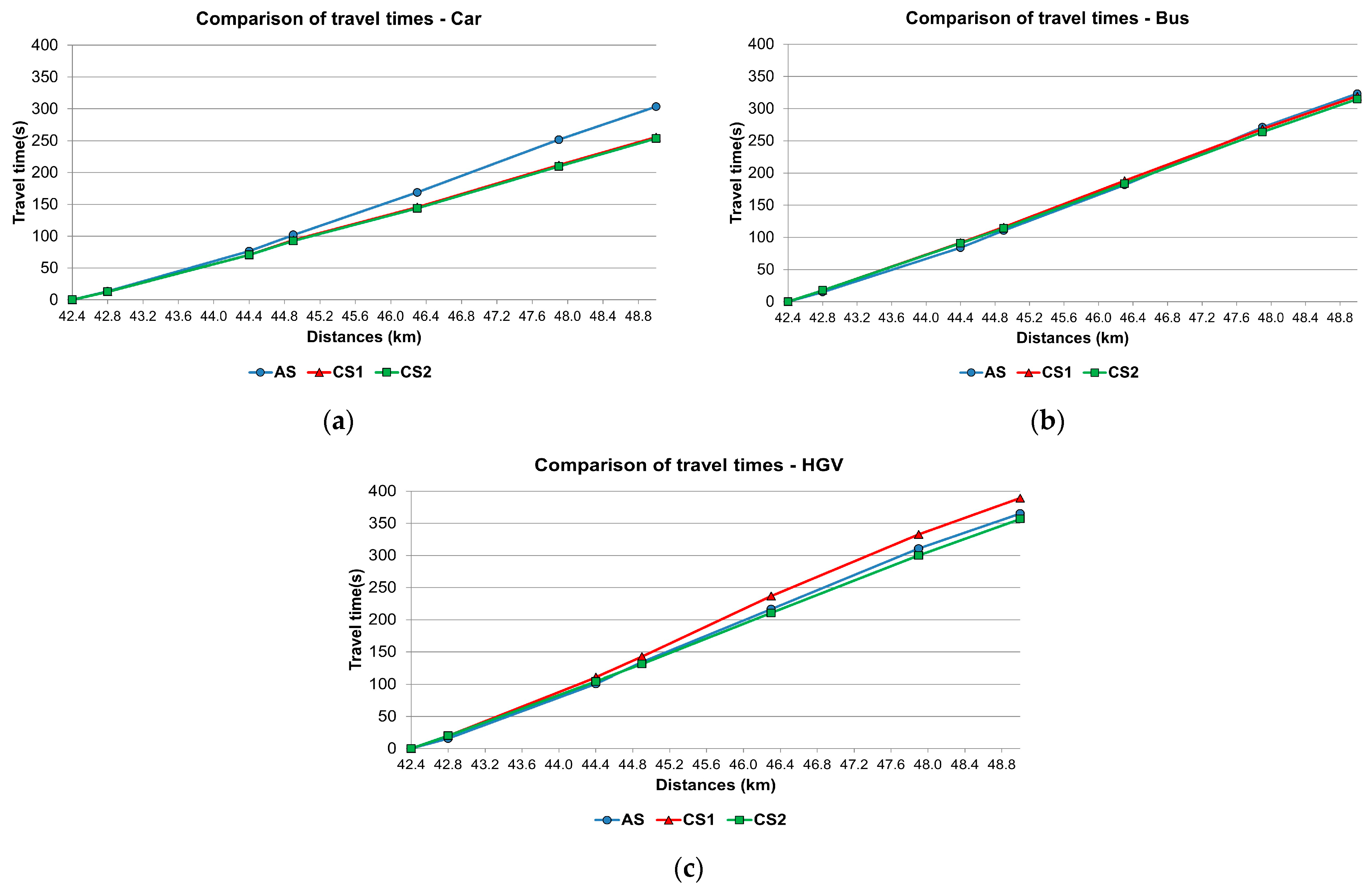
Shown in Figure 7 and Figure 8 are the average travel times and average delay times of each vehicular category along the considered segment in the three scenarios analyzed: AS, CS1, and CS2:
The analysis of Figure 7 shows that HGVs take the longest time to travel the analyzed segment, due to their performance characteristics (mass/power ratio). Figure 7c shows, in fact, average travel time values for HGVs varying between 357 and 389 s, depending on the scenarios represented; buses, on the other hand, present an average travel time that is almost unchanged as the three scenarios vary, with a value of about 314 s (Figure 7b). From Figure 7a, it is evident that for light vehicles the average travel time changes from 303 s in the AS to about 50 s in the presence of the climbing lanes (scenarios CS1 and CS2).
This result makes clear both the interaction effects between heavy vehicles and light vehicles within the traffic flow and the benefit provided by climbing lanes (and its magnitude).
Concerning the delay times analysis, HGVs (Figure 8c) present the highest average values, varying between 88 (CS1 and CS2) and 98 s (AS), followed by buses (Figure 8b) with values varying between 50 and 57 s, depending on the scenarios analyzed, influenced by the behavior of HGVs as well. Light vehicles, on the other hand, accumulate average delay times in AS equal to 63 s (Figure 8a), queuing behind heavy vehicles. These delay times decrease by about 50 s in the alternative scenarios, reaching cumulative values of about 13 s.
The increase in travel times and, consequently, delay times in AS thus leads to a drop in the performance of both light and heavy vehicles and, consequently, also to an increase in the risk of improper maneuvers, such as hazardous overtaking. The average travel and delay times of heavy vehicles and buses in CS1 and CS2 are found to be slightly higher due to the queuing waiting time caused by finding sufficient available gaps to enter in before the ending of the climbing lanes.
Frequency histograms have been realized for travel times (Figure 9) and delay times (Figure 10) of light vehicles, too, to assess the disturbance effect of heavy vehicles (“HGVs” and Buses”) in the sections with higher longitudinal gradient. Figure 9 and Figure 10 show histograms at 42+800 km and 49+000 km:
The distribution of average travel times and delay times at the beginning of the analyzed section evidence an almost similar behavior of cars in all three scenarios (Figure 9a and Figure 10a). In contrast, the analysis of the distribution of average travel times at the final distance shows a tail of values in the AS, while it maintains a normal distribution for the CS1 and CS2 scenarios, around an average value of about 44 s (Figure 9b). Turning to the analysis of the frequency distributions of the light vehicles delay times, a similar trend can be found at the final road section, corresponding to 49+000 km: a tail of cumulative delays in AS, largely due to the presence of the heavy vehicles on the same lane. The beneficial effect of the climbing lanes, therefore, is demonstrated by the presence of a peak of delay time values close to 0 for the CS1 and CS2 scenarios (Figure 10b).

3.3. Queuing Waiting Times

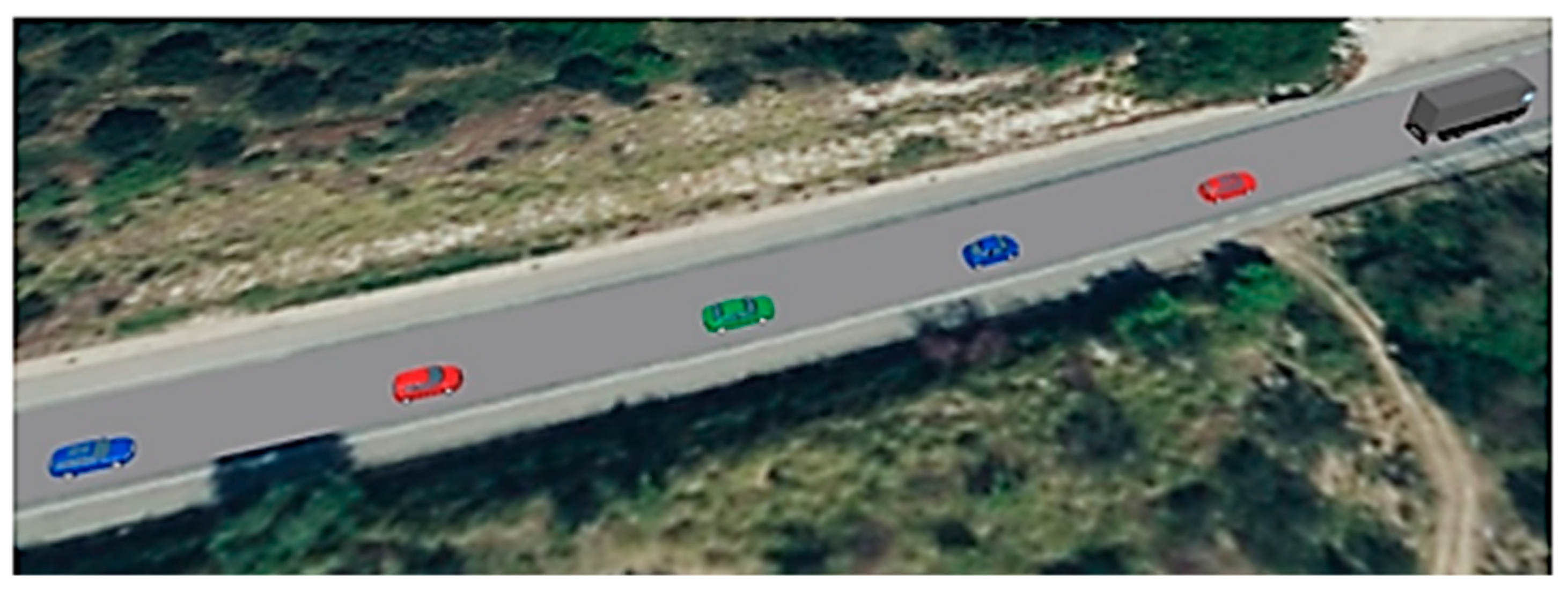
Queuing waiting time refers to the time a vehicle spends behind another vehicle before possibly performing the desired overtaking maneuver. This assessment is very important for safety purposes, as high delay times and, therefore, high queuing waiting times (Figure 11) reduce the level of service of a road and sometimes incentivize illegal overtaking maneuvers.
Queuing waiting times due to the presence of heavy vehicles (Figure 12b) have been determined in AS as the difference between the total delay time in the case where all three vehicular categories are present and the total delay time in the case where only light vehicles are present (Figure 12a).
Figure 12a shows the effect of heavy vehicles on the average delay times of light vehicles, which cause about 86% of the total delay time (63 s), while the remaining 14% is due to interactions between light vehicles only (9 s). The settings of the microsimulation software cause all heavy vehicles to travel in the climbing lanes while light vehicles travel in the main lane. In this way, there is no interaction between heavy and light vehicles, but this may not happen in real life as well, where the variables that condition driving are many and not all perfectly reproducible through a microsimulation model. For this reason, queuing waiting times have been determined, only in single-lane sections in each travel direction, for each scenario, Table 7:
The queuing waiting times in CS1 and CS2 in the sections where the climbing lanes are not present are greatly reduced when compared to the values obtained at the same distances in the AS scenario (i.e., 1.25 vs. 4.38 and 3.99 vs. 20.29). This is a further confirmation that the introduction of the auxiliary lane for slow-moving vehicles provides benefits also in the sections between them. Such a reduction in average queuing waiting time, in fact, significantly lowers the risk of non-permitted overtaking on the left. The queuing waiting times are found to be identical in the two counterfactual scenarios. The only difference lies in the fact that, having created in CS2 a single additional lane section between 42+800 km and 46+300 km, queuing waiting times are zero in the sub-section between 44+400 km and 44+900 km, providing additional functionality and safety benefits to the infrastructure.
It should be noted that, due to the software’s difficulty in simulating overtaking on roads with one lane in each direction, the travel times and delays simulated by VISSIM may probably be overestimated compared with those measurable in situ. However, it is believed that the results of the carried-out simulations are qualitatively satisfactory for the purpose of assessing the influence of heavy vehicles on light vehicles and the decay of operating conditions due to the longitudinal slope and mutual interactions between vehicles, and that they allow a comparison of possible design alternatives and a selection of the one deemed optimal.

4. Conclusions

This study has set the goal of evaluating the effects of climbing lanes on long uphill stretches of single-carriageway rural roads with one lane in each travel direction by implementing a microsimulation model in the VISSIM software. In particular, the survey has been carried out on an existing stretch of approximately 5-km length of the National Road n. 4 Via Salaria, characterized by steep gradients. On the segment between 42+800 km and 49+000 km, a series of upgrading works are planned to improve the operating conditions of the infrastructure. Three scenarios have been analyzed and compared, with the aim of identifying the optimal solution (also in terms of benefit–cost ratio): the AS referring to the rod infrastructure actual scenario, and two counterfactual scenarios, CS1 and CS2, involving three and two climbing lanes in sequence, respectively.
The implementation of a microsimulation model, calibrated and validated through the actual conditions of the analyzed segment, starts from the observation of the traffic operating conditions in AS, and then compares them with those coming from the two proposed alternatives CS1 and CS2. The consequential effects of the climbing lanes for the uphill of slow-moving vehicles were analyzed and quantified in terms of vehicle speeds, travel times and delay times, and queuing waiting times of three different vehicular classes: light vehicles, HGVs, and buses.
The obtained results, in accordance with the scientific literature, confirm the effectiveness of climbing lanes on a single-carriageway rural road with one lane in each direction as they limit the formation of “platoons,” ensuring an adequate level of service and increasing the intrinsic safety of the infrastructure [35,36]. Between the two proposed alternative scenarios, it has been demonstrated that CS2, which involves the merging of the first two additional lane sections provided in CS1, has greater benefits especially in terms of average travel speed and travel time. Moreover, from a road safety point of view, merging two climbing lanes into one results in a reduction in the number of conflict points due to the merging maneuvers of slow-moving vehicles to and from the additional lane.
This paper evaluates the beneficial effects of climbing lanes for uphill travel, which improve vehicular performances, and highlights the potential of microsimulation models in the analysis and evaluation of different traffic scenarios, through a real case study. Future research may explore issues related to road safety through a more detailed evaluation of queuing waiting times, which are often the basis of dangerous driving behaviors (e.g., hazardous overtaking) to improve driving conditions.

Author Contributions

Conceptualization, G.C. and R.G.; methodology, G.D.S. and R.G.; software, R.G.; validation, G.D.S., P.P. and G.C.; formal analysis, G.C. and R.G.; investigation, G.C.; resources, G.D.S.; data curation, R.G.; writing—original draft preparation, R.G. and P.P; writing—review and editing, G.D.S. and P.P.; visualization, G.D.S. and P.P.; supervision, G.C.; project administration, G.C. All authors have read and agreed to the published version of the manuscript.

Funding

This research received no external funding.

Data Availability Statement

Data are unavailable due to privacy and ethical restrictions.

Conflicts of Interest

The authors declare no conflict of interest.

References

  1. Al-Kaisy, A. Two-Lane Highways: Indispensable Rural Mobility. Encyclopedia 2022, 2, 625–631. [Google Scholar] [CrossRef]
  2. Cantisani, G.; Borrelli, C.C.; Del Serrone, G.; Peluso, P. Optimizing Road Safety Inspections on Rural Roads. Infrastructures 2023, 8, 30. [Google Scholar] [CrossRef]
  3. Harwood, D.; Mason, J.; Glauz, W.D.; Kulakowski, B.T.; Fitzpatrick, K. Truck Characteristics for Use in Highway Design and Operation; Appendixes, Final Report; National Academies: Washington, DC, USA, 1990; Volume 2, ISBN 1111111111. [Google Scholar]
  4. Del Serrone, G.; Cantisani, G.; Peluso, P.; Coppa, I.; Mancinetti, M.; Bianchini, B. Road Infrastructure Safety Management: Proactive Safety Tools to Evaluate Potential Conditions of Risk. Transp. Res. Procedia 2023, 69, 711–718. [Google Scholar] [CrossRef]
  5. Officials, T. A Policy on Geometric Design of Highways and Streets, 2011; AASHTO: Washington, DC, USA, 2011. [Google Scholar]
  6. Glennon, J.C. An Evaluation of Design Criteria for Operating Trucks Safely on Grades. Highw. Res. Rec. 1970, 312, 93–112. [Google Scholar]
  7. Carlsson, G. Model for Calculating the Effect of Longitudinal Profiles on the Speed of Heavy Vehicles; Statens Väginstitut: Stockholm, Sweden, 1970. [Google Scholar]
  8. Moridpour, S.; Mazloumi, E.; Mesbah, M. Impact of heavy vehicles on surrounding traffic characteristics. J. Adv. Transp. 2014, 49, 535–552. [Google Scholar] [CrossRef]
  9. Manual, H.C. Highway Capacity Manual; Transportation Research Board: Washington, DC, USA, 2000; Volume 2. [Google Scholar]
  10. Modelli di Simulazione del Traffico. Available online: http://tis.unical.it/tritone_tesi/2010-2011_4.htm (accessed on 4 May 2023).
  11. Cantisani, G.; Del Serrone, G.; Biagio, G. Di Calibration and Validation of and Results from a Micro-Simulation Model to Explore Drivers’ Actual Use of Acceleration Lanes. Simul. Model. Pract. Theory 2018, 89, 82–99. [Google Scholar] [CrossRef]
  12. Choi, S.; Suh, J.; Yeo, H. Microscopic Analysis of Climbing Lane Performance at Freeway Uphill Section. Transp. Res. Procedia 2017, 21, 98–109. [Google Scholar] [CrossRef]
  13. Ko, H.; Han, E.; Kim, K.; Park, S.; Engineering, I.Y.-K.J. Dynamic Control of Climbing Lane on Expressways. KSCE J. Civ. Eng. 2019, 23, 400–410. [Google Scholar] [CrossRef]
  14. Qin, Y.; Xiong, J.; Li, J. Driving Simulation Evaluation to Traffic Flow Characteristics and Driving Safety of Climbing Lane on a Rural Highway. J. Highw. Transp. Res. Dev. 2012, 6, 79–83. [Google Scholar] [CrossRef]
  15. Yaqin, Q.; Jian, X.; Hongqi, L.; Fengxiang, G.; Huasen, W. Driving Simulation Study of Traffic Flow Characteristics of the Climbing Lane on a Two-Lane Rural Road. In ICCTP 2009: Critical Issues in Transportation Systems Planning, Development, and Management; ASCE Library: Reston, VA, USA, 2009; Volume 358, pp. 804–811. [Google Scholar] [CrossRef]
  16. Valencia-Alaix, V. Operational Evaluation of Climbing Lanes on Steep Grades and Heavy Trucks. Transp. Res. Procedia 2020, 48, 840–884. [Google Scholar] [CrossRef]
  17. Hou, Q.; Meng, X.; Huo, X.; Cheng, Y.; Mechanics, J.L.-P.A.S. Effects of Freeway Climbing Lane on Crash Frequency: Application of Propensity Scores and Potential Outcomes; Elsevier: Amsterdam, The Netherlands, 2019. [Google Scholar]
  18. Rrecaj, A.A.; Bombol, K.M. Calibration and Validation of the VISSIM Parameters—State of the Art. Tem J. Technol. Educ. Manag. Inform. 2015, 4, 255–269. [Google Scholar]
  19. Manjunatha, P.; Vortisch, P.; Mathew, T. Methodology for the Calibration of VISSIM in Mixed Traffic. In Transportation Research Board 92nd Annual Meeting; Transportation Research Board: Washington, DC, USA, 2013. [Google Scholar]
  20. IT Ministry for Infrastructures and Transport. Ministerial Decree Nov, 5-2001, No. 6792. Norme Funzionali e Geometriche per la Costruzione delle Strade; Official Gazette of IT Republic: Rome, Italy, 2002. [Google Scholar]
  21. Cantisani, G.; Del Serrone, G. Procedure for the Identification of Existing Roads Alignment from Georeferenced Points Database. Infrastructures 2020, 6, 2. [Google Scholar] [CrossRef]
  22. Osservatorio del Traffico|Anas, S.p.A. Available online: https://www.stradeanas.it/it/le-strade/osservatorio-del-traffico (accessed on 9 May 2023).
  23. Cantisani, G.; Del Serrone, G.; Peluso, P. Reliability of Historical Car Data for Operating Speed Analysis along Road Networks. Science 2022, 4, 18. [Google Scholar] [CrossRef]
  24. Azlan, N. Overview of Application of Traffic Simulation Model. In MATEC Web of Conferences; EDP Sciences: Les Ulis, France, 2018. [Google Scholar] [CrossRef] [Green Version]
  25. Friedrich, M. A multi-modal transport model for integrated planning. In Proceedings of the 8th World Conference on Transport ResearchWorld Conference on Transport Research Society, Mumbai, India, 26–31 May 1999; Volume 2. [Google Scholar]
  26. Dorokhin, S.; Artemov, A.; Likhachev, D.; Novikov, A.; Starkov, E. Traffic Simulation: An Analytical Review. IOP Conf. Ser. Mater. Sci. Eng. 2020, 918, 012058. [Google Scholar] [CrossRef]
  27. Software per la Simulazione Dettagliata del Traffico|PTV Group. Available online: https://www.ptvgroup.com/it/soluzioni/prodotti/ptv-vissim/ (accessed on 12 May 2023).
  28. Yang, Z.; Ge, L. Research on Microscopic Traffic Simulation Model in VISSIM. DEStech Trans. Comput. Sci. Eng. 2018. [Google Scholar] [CrossRef] [PubMed] [Green Version]
  29. PTV, A.G. PTV VISSSIM 10 User Manual; PTV AG: Karlsruhe, Germany, 2018. [Google Scholar]
  30. Pontius, R.G.; Pacheco, P. Calibration and Validation of a Model of Forest Disturbance in the Western Ghats, India 1920–1990. GeoJournal 2004, 61, 325–334. [Google Scholar] [CrossRef]
  31. Guidelines for Applying Traffic Microsimulation Modeling. Available online: https://scholar.google.com/scholar?hl=it&as_sdt=0%2C5&q=Guidelines+for+Applying+Traffic+Microsimulation+Modeling+Software&btnG= (accessed on 2 May 2023).
  32. Gallelli, V.; Iuele, T.; Vaiana, R.; Vitale, A. Investigating the Transferability of Calibrated Microsimulation Parameters for Operational Performance Analysis in Roundabouts. J. Adv. Transp. 2017, 2017, 3078063. [Google Scholar] [CrossRef]
  33. Gallelli, V.; Guido, G.; Vitale, A.; Vaiana, R. Effects of Calibration Process on the Simulation of Rear-End Conflicts at Roundabouts. J. Traffic Transp. Eng. 2019, 6, 175–184. [Google Scholar] [CrossRef]
  34. Santos, L.P. Sensitivity Analysis of Vissim Driver Behavior Parameters on Safety of Simulated Vehicles and their Interaction with Operations of Simulated Traffic. In 92nd Annual Meeting of the Transportation Research Board; Transportation Research Board: Washington, DC, USA, 2013. [Google Scholar]
  35. Zlatkovic, M.; Ksaibati, K.; Haq, M.T. Final Report Wy-2002f Safety and Operational Analysis with Mitigation; University of Wyoming: Laramie, WY, USA, 2020. [Google Scholar]
  36. Ekneligoda, D.M. Study of the Performance of Passing and Climbing Lanes along Colombo—Rathnapura—Wellawaya—Batticolo Road Study of the Performance of Passing and Climbing Lanes along Colombo—Rathnapura—Wellawaya—Batticolo Road. Ph.D. Thesis, University of Moratuwa, Moratuwa, Sri Lanka, 2020. [Google Scholar]
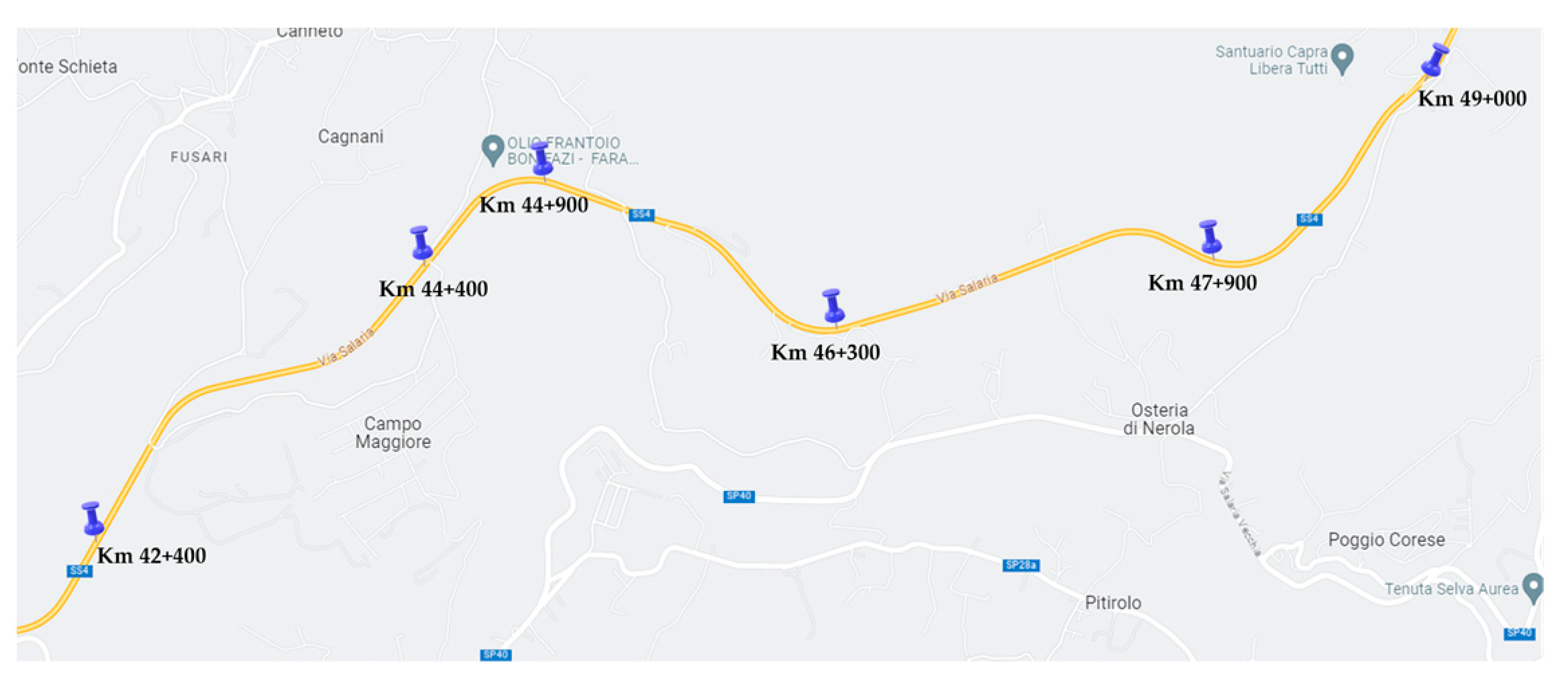
Figure 1. Horizontal layout of the studied section [Google Maps].
Vehicles 05 00041 g001
Figure 2. Vertical alignment of the road section considered Via Salaria (a) CS1, that includes three climbing lanes; (b) CS2, that includes just two climbing lanes.
Vehicles 05 00041 g002
Figure 3. Point-based sensors analyzed, falling within the examined section.
Vehicles 05 00041 g003
Figure 4. Comparison of real and simulated speeds in the two directions of travel, during the peak hour of the morning or afternoon, on weekdays, and weekend: (a) Ascending direction, morning, weekday; (b) Ascending direction, afternoon, weekday; (c) Descending direction, morning, weekday; (d) Descending direction, afternoon, weekday; (e) Ascending direction, morning, weekend; (f) Ascending direction, afternoon, weekend, (g) Descending direction, morning, weekend; (h) Descending direction, afternoon, weekend.
Vehicles 05 00041 g004
Figure 5. Average speeds comparison in the three analyzed scenarios (AS, CS1, e CS2), for each vehicular category: (a) Car; (b) Bus; (c) HGV.
Vehicles 05 00041 g005
Figure 6. Light vehicle speed distributions in the 3 scenarios: (a) 42+800 km; (b) 49+000 km.
Vehicles 05 00041 g006
Figure 7. Average travel times along the considered segment in the three scenarios analyzed (AS, CS1, and CS2) for each vehicular category: (a) Car; (b) Bus; (c) HGV.
Vehicles 05 00041 g007
Figure 8. Average delay times along the considered segment in the three scenarios analyzed (AS, CS1, and CS2) for each vehicular category: (a) Car; (b) Bus; (c) HGV.
Vehicles 05 00041 g008
Figure 9. Light vehicles travel times frequency histograms in the three scenarios analyzed: (a) 42+800 km; (b) 49+000 km.
Vehicles 05 00041 g009
Figure 10. Light vehicles delay times frequency histograms in the three scenarios analyzed: (a) 42+800 km; (b) 49+000 km.
Vehicles 05 00041 g010
Figure 11. Queuing waiting times of light vehicles behind an HGV (VISSIM).
Vehicles 05 00041 g011
Figure 12. Estimated light vehicles queuing times in AS: (a) with and without heavy vehicles; (b) final curve obtained by subtraction.
Vehicles 05 00041 g012
Table 1. Peak hour traffic flows during weekdays and weekends.
Peak Hour Traffic Flow (veh/h)WeekdayWeekends
Ascendant morning480410
Ascendant afternoon380320
Descendant morning420390
Descendant afternoon400420
Table 2. Vehicular sub-categories distribution in the 2 travel directions.
Vissim Typological
Classification
Famas 9+1 Typological
Classification
% dir. A% dir. D
Carmotorcycles, cars, vans9596
Heavy Goods Vehicle—HGVcar trailers, trucks, articulated trucks, road trains43
Busbuses11
Table 3. Global parameters setting for the model calibration.
Default SettingsAdopted Settings
Simulation resolution; Time steps (seconds)/seconds of simulation1010
Simulation speed1010
Vehicular composition (Vehicular types; speed distributions desired; percentage of each vehicular class of total flow)100 (Car; 50 km/h; 0.980)
200 (HGV, 50 km/h; 0.020)
100 (Car; 90 km/h; 0.950)
200 (HGV; 75 km/h; 0.040)
300 (Bus; 75 km/h; 0.010)
Vehicular Fleet-Anas control unit data
Vehicular classesCar, HGV, Bus, Tram, Pedestrian, BicycleCar, HGV, Bus
Table 4. Wiedemann 99 model for the “car following” parameters.
ParametersDescriptionUnitDefault Value
CC0Standstill distancem1.50
CC1Gap time distributions0.90
CC2‘Following’ distance oscillationm4.00
CC3Threshold for entering ‘Following’s−8.00
CC4Negative speed differencem/s−0.35
CC5Positive speed differencem/s0.35
CC6Distance dependency of oscillation1/(ms)11.44
CC7Oscillation accelerationm/s20.25
CC8Acceleration from standstillm/s23.50
CC9Acceleration at 80 km/hm/s21.50
Table 5. Lane changing parameters.
ParametersUnitDefault Values
OwnTrailing Vehicle
Maximum decelerationm/s23.502.50
−1 m/s2 per distancem80.0080.00
Accepted decelerationm/s21.001.00
Waiting time before diffusions60.00
Minimum clearance (front/rear)M0.50
Safety distance reduction factor-1.00
Maximum deceleration for cooperative brakingm/s22.50
Table 6. Chi-square (χ2) goodness of fit during weekdays and weekends.
Chi-Square ( χ 2 ) Goodness of Fit WeekdayWeekends
Ascendant morning11.112.9
Ascendant afternoon13.07.8
Descendant morning6.85.5
Descendant afternoon8.96.8
Table 7. Average queuing waiting times in the 3 scenarios, AS, CS1 and CS2.
Distances (km)Queuing Waiting Times (s)
Starting Point Ending PointASCS1CS2
42+40042+8000.080.050.05
42+80044+4004.93--
44+40044+9004.381.25-
44+90046+30015.61--
46+30047+90020.293.993.99
47+90049+0008.82--
Disclaimer/Publisher’s Note: The statements, opinions and data contained in all publications are solely those of the individual author(s) and contributor(s) and not of MDPI and/or the editor(s). MDPI and/or the editor(s) disclaim responsibility for any injury to people or property resulting from any ideas, methods, instructions or products referred to in the content.