Article

Optimizing Nonlinear Lateral Control for an Autonomous Vehicle

by
Lorien Revueltas
1,
Omar-Jacobo Santos-Sánchez
2,
Sergio Salazar
1,* and
Rogelio Lozano
1,3
1
CINVESTAV, Mexico 07360, Mexico
2
Research Center in Information Technology and Systems “CITIS-ICBI”, Autonomous University of the State of Hidalgo, Pachuca 42184, Mexico
3
Universite de technologie de Compiegne, CNRS, Heudiasyc, CS 60 319 Compiegne, France
*
Author to whom correspondence should be addressed.
Vehicles 2023, 5(3), 978-993; https://doi.org/10.3390/vehicles5030053
Submission received: 3 July 2023 / Revised: 28 July 2023 / Accepted: 7 August 2023 / Published: 10 August 2023

Abstract

:
The lack of general algorithms for the control of nonlinear systems is a generalized problem, especially when attempting to stabilize systems such as ground vehicles, which have uncertainties and are usually linearized under the assumption of small angles. To solve this problem, in this work, the implementation of a suboptimal discrete control is developed to stabilize an autonomous automobile. We assume the system is affine for the optimization procedure of finite horizon that allows us to find a solution while avoiding solving the Ricatti-type equation, commonly encountered in this kind of algorithm. This procedure is applied to the dynamical model of the lateral displacement and orientation errors of the vehicle that was discretized through the method of Euler. These nonlinear models discretized to compute a bounded control. The control is tested in different simulated scenarios to show the efficiency of the system for solving typical tasks for the path planning of an autonomous vehicle.

1. Introduction

Driving a vehicle is a very complex task, that requires the full concentration of the driver. To enable a computer system to replace the human driver effectively, it must be equipped with multiple sensors and control algorithms for various aspects of a land vehicle’s architecture. Many systems have been developed with different approaches to solve a variety of circumstances, from urban driving to highways, where the number of other vehicles, the presence of objects, and the velocity of the car are incredibly diverse. These studies concern autonomous vehicles, which are able to travel long distances without any human assistance beyond the supervision of the correct function of the developed systems. Nevertheless, different problems can be solved and improved, and current research is devoted to enhancing the response of the vehicle. This is carried out by using new control algorithms applied to nonlinear models or new approaches that enhance the measurements and reduce uncertainties. Some of the results obtained are described in the next paragraphs. Their proposed solutions often included a combination of different types of controllers, observers, estimators, adaptive control, or fuzzy control.
Jin et al. [1] created an observer for the side-slip angle with road friction adaptation. Their proposition also relies on using discrete time control. In each iteration for the state and parameter estimation, the optimization problem is solved. The integration of a continuous sensor is fused with the discrete time control.
Xiong et al. [2] designed another slip angle estimator that uses high-fidelity Inertial Measurement Unit (IMU) information, and the attitude estimator created a method such that the accumulated error is eliminated. The attitude estimator information is gathered by two estimators based on the vehicle dynamic model. This algorithm includes a delay estimation and prediction to improve the performance, given that it takes time to detect abnormal estimations created by a critical steering in the vehicle.
Shao et al. [3] reduce the risk of rollover in an efficient and robust manner, using a slip angle observer with sliding mode in combination with a switching term that depends on a linear observer. They included an adaptive sliding mode control in which, in order to have compensated for the system uncertainties, the gain is adaptively tuned. This is used in the steer-by-wire system that must be equipped to decrease lateral acceleration in the vehicle. The controller for the rollover must be properly adjusted with the other control system to prevent potential incidents such as collisions.
Wang et al. [4] used two models combined, the vehicle model and the vision model. This was made to increase the robustness of the estimation of the body slip-angle. They included an inter-sample compensation and multi-rate Kalman filter to improve the accuracy of the estimator strategy that constrains the error in the heading and the lateral position. This inter-sample period is created for the difference in the sampling time of a regular camera and the period of the motor of the vehicle, the latter being faster than the former. Their controller for reference tracking considers two degrees of liberty.
Zhang [5] considered a robot arm to steer the hand wheel with a lateral tracking control strategy that was proposed using a cost function. He obtained a strategy that constrains the error in the heading and the lateral position. His strategy also includes active acceleration and braking. The robustness in performance was achieved through the design made by linear matrix inequalities while a scheduling gain approach is used for the robustness in the control system to the time-changing variables.
Tagne et al. [6], for lateral control, designed a higher-order sliding mode control. The steering angle is used as the control input and the error in the lateral displacement is the output. Their work uses the super-twisting algorithm to ensure the controller works in high velocities, since it reduces the lateral displacement. Using high-order sliding mode and the super-twisting algorithm allows for robust control against nonlinearities and parameter uncertainties, while also reducing chattering.
Fekih et al. [7] developed a fault-tolerant control based on Linear-Quadratic Regulator (LQR) control with a feed-forward gain for path tracking. In the case of parameter variations or uncertainties, the proposal includes a weight adjustment algorithm. They also incorporated an observer to detect and identify sensor faults through sensor fusion, along with a fault-tolerant controller to ensure stability.
Wang et al. [8] proposed the union of two methods, the first one is a tire force distribution rule, and the second one is a path-tracking controller with a time-varying Model Predictive Control (MPC). In this case, the strong nonlinearities and coupling of the dynamics of the tire are described with a UNiTire model that is combined with slip conditions; however, the model for the controller was linearized using Taylor expansion.
Moreno-Gonzalez et al. [9] used the paradigm known as Model- Free control for a control that is decoupled in its architecture. The Model-Free framework reduces the dynamics of a complex system with strong nonlinearities to a simple model with online updating, ensuring stability in different velocities and dynamic constraints. The method was evaluated based on trajectory tracking, stability, safety, and passenger comfort.
Barari et al. [10] proposed a two-layer hierarchical control strategy for coordinated control. The upper layer uses a self-tunable super-twisting sliding mode control to handle parametrical uncertainties, while the lower layer employs Model Predictive Control (MPC) for control action in active front steering and direct yaw moment control. The design takes into account parametric uncertainties in mass, cornering stiffness of tires, and moment of inertia.
The hierarchical architecture used by G. Chen et al. [11] to achieve better performance and energy savings includes, among other parts, a sliding mode control for the yaw moment and the total force, an energy-efficiency optimization to reduce losing power, and a blended strategy for controlling the brake. The energy optimization in the motor also produces an energy recovery using a motor efficiency map and, to reduce losing power as a consequence of the tire sideslip, the lateral force is decreased. The steering angle is designated on the basis of the Ackerman steering theorem [12]. This proposition uses a linear model for the accelerations and a nonlinear equation for the control of the steering angle. In the area of fuzzy systems, Nguyen et al. [13] used the fuzzy static output developed with Fuzzy Lyapunov Function and the non-parallel distributed compensation to counteract the uncertain behaviors from dynamics of the vehicle and specifically the forces acting in the tires. This approach involves reformulating the control problem as an optimization problem using convexification techniques. The control constraints are expressed as linear matrix inequalities, which can be efficiently solved using semidefinite programming techniques.
Taghavifar et al. [14], proposed a fuzzy control that was implemented in the form of a fuzzy neural network to enhance the path-tracking performance. The control is adaptive and based on the design of exponential and sliding modes in the approach of fuzzy neural networks. The chattering is eliminated using a convergence control law adjusted with the base on the variable exponential sliding manifold. A hierarchical controller is included in the design for the stability of the closed-loop system, the controller was obtained using a Lyapunov approach.
However, all the approaches mentioned above were not designed using the nonlinear model of the system. The vehicle model is often linearized through the consideration of small angles. Nevertheless, the model of the vehicle has strong nonlinearities, as can be seen in the model of the bicycle described by Rajamani [12].
The present paper aims to design a control algorithm that effectively incorporates the nonlinearities inherent in the vehicle model, thereby enhancing the performance of the closed-loop system. The proposed approach introduces a suboptimal control strategy for the vehicle, leveraging information from lateral position and orientation errors. Its primary contribution involves the development of a nonlinear discrete suboptimal control, utilizing the nonlinear dynamical model of the vehicle. It is crucial to highlight that synthesizing an optimal controller for nonlinear systems, be they discrete or continuous, necessitates solving the Bellman equation, which is generally unknown. However, the proposed controller design adeptly circumvents the need to solve the Bellman equation within the suboptimal nonlinear discrete algorithm. Instead, a minimization procedure is employed to ensure the achievement of local minimum, ensuring efficient control performance. To evaluate the effectiveness of the proposed controller, extensive numerical simulations are conducted. The chosen tests include a lane-keeping assessment, where the vehicle is required to stay centered within a lane or realign itself with a new center after changing lanes. This capability enables the vehicle to avert collisions with surrounding vehicles, objects, and structures, enhancing safety and efficiency. Additionally, a velocity profile tracking test is performed, a key component of path planning for guiding a vehicle from point A to point B along a specific route. These simulations demonstrate the robustness and practical applicability of the proposed control strategy in critical real-world scenarios.

2. Materials and Methods

The methods used to obtain the results exposed in the next section can be divided into two categories. The first category is the mathematical development of the equations that describe the control with the model of the vehicle in discrete time, and the second is the description of how to make the mathematical simulation in Matlab Simulink 2022a.
The mathematical development of the control starts from the definition of controllability for a pair of points in a discrete-time system and proceeds to describe how this applies in the case of affine systems when trying to find an optimal control that minimizes certain performance indexes. Then, the suboptimal is adapted to the model of the vehicle, which has to be discretized for this purpose. The description of the settings for the mathematical simulations includes the parameters used for the model and the necessary parameters for the control. It also included the proof of the properties of the control parameters, which are defined to need these properties.

2.1. Suboptimal Control

2.1.1. Optimization Procedure of Finite Horizon

We remind the reader that the controllability of discrete systems has the following basic definition.
Definition 1. 
The pair x o , x 1 is said to be controllable if an admissible control u ( k ) exits and, when applied to the system defined by x ( k + 1 ) = f x ( k ) , u ( k ) takes the system from x 0 to x 1 in N finite number of steps. Where x ( k ) , f . , . R n , u ( k ) R m .
To be admissible, a control must be bounded. According to the definition, one of the problems for nonlinear discrete systems is finding the N step in which the state finally converges to x 1 . In the present paper, we consider that the value of the step will be changed in the case that the system state is not equal to the final state x 1 ; in other words, the number of steps is fixed.

2.1.2. Affine Systems Suboptimal Discrete Nonlinear Control

The discrete affine system is described below
x ¯ ( k + 1 ) = f 0 ( x ¯ k ) + f 1 x ¯ k u k ,
where k = 0 , 1 , , N , x ¯ k , f 0 ( x ¯ k ) R n , f 1 x ¯ k R n × m and u ( k ) R m . The sampling time for this discrete system is defined as T s . The problem considered here is to find the control input u ( k ) that minimizes the following quadratic performance index when applied to the system:
J = 1 2 x ¯ T N S x ¯ ( N ) + 1 2 k = 0 N 1 x ¯ T k Q x ¯ ( k ) + u T ( k ) R u ( k ) ,
where t f = T s N is the finite time horizon, N some integer representing the step, matrices Q , S 0 and R > 0 have the appropriate dimensions, and they are used as weighting matrices for the relative importance of the values of x ¯ ( k ) and u ( k ) . The higher the values of the matrices elements, the more significant the corresponding x ¯ ( k ) and u ( k ) are. Suppose that the Definition 1 is satisfied by a pair of points x 0 , x t f of the nonlinear discrete system (1). The main ideas of the dynamic programming approach exposed below, was proposed originally in [15]. This approach was applied to the Unmanned Aerial Vehicle (UAV) in [16], to an Autonomous Soaring UAV in [17] and to an hybrid exoskeleton in [18].
Theorem 1. 
Consider the quadratic performance index (2) and the system in Equation (1). The suboptimal sequence u ˜ N k , which makes the performance index reach a local minimum, is
u ˜ N k = f 1 T x ¯ N k Q f 1 x ¯ N k + R 1 f 1 T x ¯ N k Q f 0 x ¯ N k ,
for all k = 2 N , , N , where matrices Q and R are symmetric positive semidefinite.
Proof. 
First, consider the following definition:
J N , N * = 1 2 x ¯ T N S x ¯ ( N )
The term is independent of the control law u ( N ) at the discrete time N. Then, it receives the name of the optimal value of J at the discrete time N. The definition of the following step is
J N 1 , N * = min u N 1 1 2 x ¯ T N S x ¯ ( N ) + 1 2 x ¯ T N 1 Q x ¯ ( N 1 ) + 1 2 u T ( N 1 ) R u ( N 1 ) = min u N 1 J N , N * + 1 2 x ¯ T N 1 Q x ¯ ( N 1 ) + 1 2 u T ( N 1 ) R u ( N 1 ) ,
Through the state space equation given by (1) the computed value of the state x ¯ ( N ) is
J N 1 , N * x ¯ N 1 , u N 1 = min u N 1 1 2 f 0 ( x ¯ N 1 ) + f 1 x ¯ N 1 u N 1 T S · · f 0 ( x ¯ N 1 ) + f 1 x ¯ N 1 u N 1 + + 1 2 x ¯ T N 1 Q x ¯ ( N 1 ) + 1 2 u T ( N 1 ) R u ( N 1 )
The minimum value of J N 1 , N will be found as the next step, consequently
u * N 1 = f 1 T x ¯ N 1 S f 1 x ¯ N 1 + R 1 f 1 T x ¯ N 1 S f 0 x ¯ N 1 ,
The term f 1 T x ¯ N 1 S f 1 x ¯ N 1 + R 1 exists as long as the matrix R > 0 . The control algorithm given by (7), as can be seen, turns out to be the optimal control, since
2 J N 1 , N x ¯ N 1 , u N 1 2 u N 1 = R > 0
The existence of the minimum is verified due to the strong convexity of the right-hand side of (6) to u N 1 . For the step N 2 , in light of the fact that the value of u * N 1 has been the optimal value for the step N 1 , and in accordance to the optimality principle of Bellman, this control formulates the optimal value for x ¯ N 1 . Subsequently, for this step N 2
J ˜ N 2 , N x ¯ N 2 , u N 1 , u N 2 = min u N 1 , u N 2 1 2 x ¯ N T S x ¯ N + + 1 2 x ¯ T N 1 Q x ¯ ( N 1 ) + 1 2 x ¯ T N 2 Q x ¯ ( N 2 ) + 1 2 u T ( N 1 ) R u ( N 1 ) + 1 2 u T ( N 2 ) R u ( N 2 )
We observe a relation, where the terms requiring x ¯ N m always rely on the control u N m 1 . According to this relation, x ¯ N relies on u N 1 , x ¯ N 1 relies on u N 2 , and so on. However, the term u N 1 found before is the optimal control and x ¯ N 1 is derived from the state Equation (1). Subsequently,
J ˜ N 2 , N x ¯ N 2 , u N 2 = min u N 2 1 2 x ¯ N T S x ¯ N + 1 2 f 0 ( x ¯ N 2 ) + + f 1 x ¯ N 2 u N 2 T Q f 0 ( x ¯ N 2 ) + + f 1 x ¯ N 2 u N 2 + 1 2 x ¯ T N 2 Q x ¯ ( N 2 ) + + 1 2 u T ( N 1 ) R u ( N 1 ) + 1 2 u T ( N 2 ) R u ( N 2 )
Now, to obtain the suboptimal control u N 2 , we make use of this last equation in this step, avoiding the very complex problem of having a Riccati-type equation in the discrete domain. However, note that (10), with regard to u N 2 , is strongly convex, guaranteeing that a minimum exists. Nevertheless, instead of the optimal value of u N 2 , we have an approximation. The reason for this is that, in order to find the true optimal control signal u N 2 , the Riccati-type equation has to be solved first, applying the solution to the nonlinear discrete model, which is hard to find. We used the above procedure to find the suboptimal control for N 2 .
u ˜ N 2 = f 1 T x ¯ N 2 Q f 1 x ¯ N 2 + R 1 f 1 T x ¯ N 2 Q f 0 x ¯ N 2
Considering the development described, we can determine that the general equations are
u ˜ N k = f 1 T x ¯ N k Q f 1 x ¯ N k + R 1 f 1 T x ¯ N k Q f 0 x ¯ N k ,
J ˜ N k , N x ¯ N k , u N k = J ˜ N k + 1 , N + 1 2 x ¯ T N k Q x ¯ ( N k ) + u ˜ T ( N k ) R u ˜ ( N k ) ,
for all k = 2 , , N . Reaching the minimal value of the performance index (2) is ensured by the suboptimal sequence obtained through these steps; see Equation (8). □

2.1.3. Suboptimal Control of the Land Vehicle

Consider the following mathematical model proposed in terms of the lateral and orientation errors with respect to the lane [12]:
m e ¨ 1 V x ψ ˙ d e s = 2 C α f δ f 1 2 C α r f 2 I z e ¨ 2 = 2 C α f f f 1 + 2 C α r r f 2 ,
where
f 1 = arctan e ˙ 1 V x e 2 + f e ˙ 2 + ψ ˙ d e s V x f 2 = arctan e ˙ 1 V x e 2 r e ˙ 2 + ψ ˙ d e s V x
The model is illustrated in Figure 1. Model variables can be consulted in the Table 1.
Now, we define the vector state as
x = x 1 x 2 x 3 x 4 T x 1 = e 1 , x 2 = e ˙ 1 , x 3 = e 2 , x 4 = e ˙ 2 , u = δ ,
then
x · = f ˜ 0 ( x ) + f ˜ 1 u ,
where
x ˙ = x ˙ 1 x ˙ 2 x ˙ 3 x ˙ 4 f ˜ 0 ( x ) = x 2 1 m η 1 m μ V x ψ ˙ d e s x 4 f I z η + r I z μ f ˜ 1 = 0 2 C α f m 0 2 C α f f I z η = 2 C α f arctan x 2 V x x 3 + f ( x 4 + ψ ˙ d e s ) V x μ = 2 C α r arctan x 2 V x x 3 r ( x 4 + ψ ˙ d e s ) V x
According to the approximation of Euler, for x ¯
x ¯ · x ¯ k + 1 x ¯ k T s ,
as before the sampling time is T s
x ¯ k + 1 = T s f ¯ 0 ( x ¯ k ) + x ¯ k f 0 ( x ¯ k ) + T s f ¯ 1 f 1 u k ,
where k = 0 , 1 , 2 , 3 , , then
x ¯ k + 1 = f 0 ( x ¯ k ) + f 1 u k ,
where
f 0 ( x ¯ k ) = T s x 2 k + x 1 k 1 m η ( k ) 1 m μ ( k ) T s V x ψ ˙ d e s + x 2 k T s x 4 k + x 3 k f I z η ( k ) + r I z μ ( k ) + x 4 k f 1 T = 0 2 m T s C α f 0 2 I z f T s C α f η ( k ) = 2 T s C α f arctan x 2 k V x x 3 k + f ( x 4 k + ψ ˙ d e s ) V x μ ( k ) = 2 T s C α r arctan x 2 k V x x 3 k r ( x 4 k + ψ ˙ d e s ) V x
According to the control given by (7), the suboptimal control in the discrete time N 1 , as a function of the error x ˜ = x x t f , is
u * N 1 = T T S T + R 1 T T S f 0 ( x ¯ N 1 ) ,
where
T = 0 2 m T s C α f 0 2 I z f T s C α f S = s 11 s 12 0 0 s 21 s 22 0 0 0 0 s 33 s 34 0 0 s 43 s 44 f 0 ( x ¯ N 1 ) = T s x ˜ 2 N 1 + x ˜ 1 N 1 1 m η ˜ ( N 1 ) 1 m μ ˜ ( N 1 ) a ˜ 1 ( N 1 ) T s x ˜ 4 N 1 + x ˜ 3 N 1 f I z η ˜ ( N 1 ) + r I z μ ˜ ( N 1 ) + x ˜ 4 N 1 η ˜ ( N 1 ) = 2 T s C α f arctan b ˜ 1 ( N 1 ) ) + f ( x ˜ 4 N 1 + ψ ˙ d e s ) V x μ ˜ ( N 1 ) = 2 T s C α r arctan b ˜ 1 ( N 1 ) r ( x ˜ 4 N 1 + ψ ˙ d e s ) V x a ˜ 1 ( N 1 ) = T s V x ψ ˙ d e s + x ˜ 2 N 1 , b ˜ 1 ( N 1 ) = x ˜ 2 N 1 V x x ˜ 3 N 1 ,
then
u * ( N 1 ) = m 2 I z 2 R m 2 I z 2 + 4 s 44 m 2 f 2 T s 2 C α f 2 + 4 s 22 I z 2 T s 2 C α f 2 2 m s 21 T s C α f x ˜ 1 ( N 1 ) + + T s x ˜ 2 N 1 + 2 m s 22 T s C α f [ x ˜ 2 N 1 T s V x ψ ˙ d e s 1 m η ˜ ( N 1 ) 1 m μ ˜ ( N 1 ) + 2 I z f s 43 T s C α f x ˜ 3 N 1 + x ˜ 4 T s N 1 2 I z f s 44 T s C α f 1 I z r μ ˜ ( N 1 ) + 1 I z f η ˜ ( N 1 ) x ˜ 4 N 1 ,
for N k , where k = 2 , 3 , , N , we have that
u ˜ N k = T T Q T + R 1 T T Q f 0 ( x ¯ N k ) ,
where
Q = q 11 q 12 0 0 q 21 q 22 0 0 0 0 q 33 q 34 0 0 q 43 q 44 f 0 ( x ¯ N k ) = T s x ˜ 2 N k + x ˜ 1 N k 1 m η ˜ N k 1 m μ ˜ ( N k ) a ˜ 1 ( N k ) T s x ˜ 4 N k + x ˜ 3 N k f I z η ˜ N k + r I z μ ˜ ( N k ) + x ˜ 4 N k η ˜ N k = 2 T s C α f arctan b ˜ 1 ( N k ) + f ( x ˜ 4 N k + ψ ˙ d e s ) V x μ ˜ ( N k ) = 2 T s C α r arctan b ˜ 1 ( N k ) r ( x ˜ 4 N k + ψ ˙ d e s ) V x a ˜ 1 ( N k ) = T s V x x ˜ 4 N k + x ˜ 2 N k b ˜ 1 ( N k ) = x ˜ 2 N k V x x ˜ 3 N k ,
then
u * N k = m 2 I z 2 R m 2 I z 2 + 4 q 44 m 2 f 2 T s 2 C α f 2 + 4 q 22 I z 2 T s 2 C α f 2 2 m q 21 T s C α f x ˜ 1 N k + + x ˜ 2 T s N k + 2 m q 22 T s C α f x ˜ 2 N k T s V x ψ ˙ d e s 1 m η ˜ ( N k ) + + 1 m μ ˜ ( N k ) + 2 I z f q 43 T s C α f x ˜ 3 N k + x ˜ 4 T s N k 2 I z f q 44 T s C α f 1 I z r η ˜ ( N k ) + 1 I z f μ ˜ ( N k ) x ˜ 4 N k ,
for k = 2 , 3 , N . Notice that S and Q have to be positive semidefinite matrices (and symmetric), so e i g S and e i g Q are positive and real, and q 12 = q 21 , q 34 = q 43 , s 12 = s 21 , s 34 = s 43 .

2.2. Numerical Simulation

2.2.1. Configuration of Numerical Simulations

Two scenarios of simulation were used to illustrate the response of the proposed suboptimal control. Both are implemented in Matlab Simulink with a velocity of V x = 30 m/s. The first scenario is a lane-keeping task, starting with a lateral error of 1 m and the model is expected to reach e 1 = 0 m with the action of the suboptimal control. The listed parameters in Table 2 were used for the lateral model in the simulation.
Furthermore, the Q matrix must be selected to be positive-definite, and the same holds for the R matrix. These matrices have been selected by trial and error and are given:
Q = 2.5 0.8 0 0 0.8 0.3 0 0 0 0 5.25 0.2 0 0 0.2 0.3 , R = 1
To recreate the conditions of a lane-keeping task in the environment of Matlab Simulink, we used the block model shown in Figure 2. In the model, the principal blocks are the Lateral Model, Suboptimal Control, and ψ d e s . The Lateral Model block contains the equations of the lateral dynamics of the vehicle in discrete time, Equations (14) and (15). The Suboptimal control block includes the proposed suboptimal control Equation (28). And the ψ d e s block was added to have the possibility of changing the desired orientation in accordance to the kind of road that will be simulated, but in this case, since we have a straight road, the value returned from this block is zero. The parameters from Table 1 are added in the Lateral Model Bloc and in the Suboptimal control block because these parameters were used in the equations mentioned before. The parameter t s , also known as the sampling time, is set to be equal to 0.01 s. The simulation is set to use fixed time steps, to introduce t s as a constant and avoid the necessity of creating a function to introduce the sampling time to the model. The block with the mathematical expression of 1 z is the representation of the time delay that allows us to move from x ( n + 1 ) to x ( n ) . The rest of the blocks are there to show the results of the different variables ( e 1 , e ˙ 1 , e 2 , e ˙ 2 , and u ( N ) ).
For the second test implemented, which is the tracking of a velocity profile, we added another two blocks, the first one is to create the velocity profile designed for this test. This profile starts at v ( 0 ) = 0 m/s and increments smoothly until reaching the velocity of v = 2 m/s when the time stamp is equal to 20 s, remains in the velocity of v = 2 m/s for 60 s, and then returns to v = 0 m/s during the next 20 s. The other block is for integrating the signal to be used in the discrete model. The Block Model for the second test is shown in Figure 3. This test uses the same parameters as before including, the fixed time step for the solver.

2.2.2. Properties of Matrices Q and R

The necessity of having positive definite matrices Q and R was established in the development of the equations for the suboptimal control. This section presents the proof that the selected Q and R are positive definite.

2.2.3. Symmetry of Matrices Q and R

For a matrix to be positive definite, first it has to be symmetric.
Definition 2. 
A matrix B is symmetric if it is equal to its transpose [19].
B = B T
Since Matrix R is of size 1 × 1 , then R is equal to its transpose R = R T . For matrix Q,
Q = 2.5 0.8 0 0 0.8 0.3 0 0 0 0 5.25 0.2 0 0 0.2 0.3 ,
the values q 12 = q 21 = 0.8 , q 34 = q 43 = 0.2 . Then,
Q T = 2.5 0.8 0 0 0.8 0.3 0 0 0 0 5.25 0.2 0 0 0.2 0.3 ,
and Q = Q T .

2.2.4. Positive Definiteness of Matrices Q and R

To demonstrate this property, the following definition can be used.
Definition 3. 
If all the principal minors of a real and symmetric matrix B are positive, then B is a positive-definite matrix (Criterion of Sylvester) [20].
The leading principal minor is the determinant of a principal submatrix, which is formed with the first n rows and columns of B, ( | B n × n | ) [20]. There is only one principal minor for R, and it is | R 1 , 1 | = 1 . Therefore, the matrix R is positive definite.
For matrix Q, there are four principal submatrices:
Q 1 , 1 = 2.5 , Q 2 , 2 = 2.5 0.8 0.8 0.3 , Q 3 , 3 = 2.5 0.8 0 0.8 0.3 0 0 0 5.25 , Q 4 , 4 = 2.5 0.8 0 0 0.8 0.3 0 0 0 0 5.25 0.2 0 0 0.2 0.3 ,
The leading principal minors of matrix Q are
| Q 1 , 1 | = 2.5 , | Q 2 , 2 | = 0.11 , | Q 3 , 3 | = 0.58 , | Q 4 , 4 | = 0.17 ,
Being all positive, therefore, the matrix Q is positive definite.

3. Results

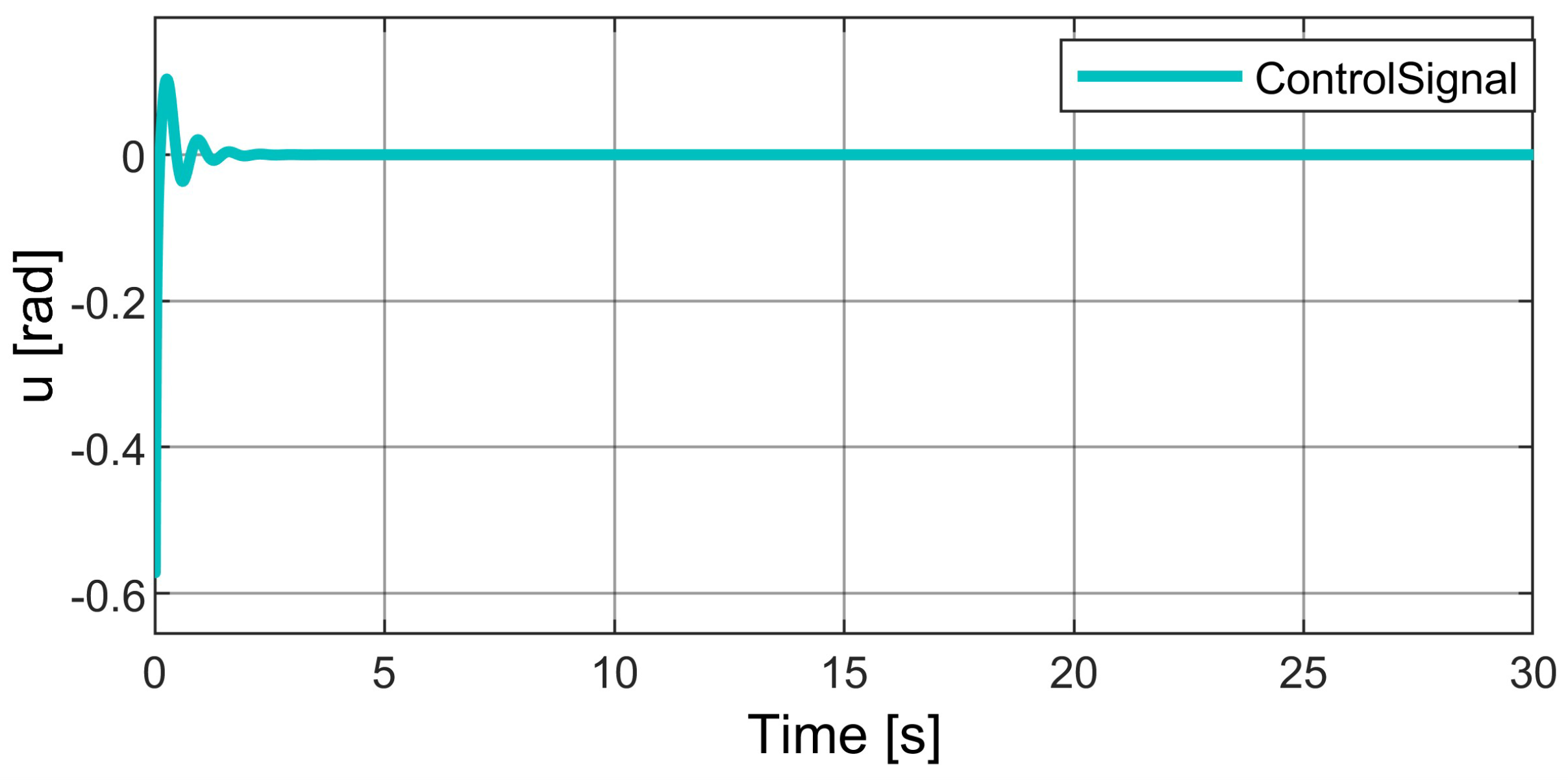
The lane-keeping test illustrates the capacity of the control to stabilize the system. It should be noticed that the error of 1 m in the lateral displacement is corrected in a short period of time, less than five seconds, and, after that, the system remains at the final state for the remainder of the time without any further lateral displacement, as can be seen in Figure 4. The suboptimal control signal keeps a small value (see Figure 5). For e 2 , it is expected to start at zero and allow the vehicle to change its orientation to correct the position and come back to zero after that. This movement is aligned with the behavior described in the variable e 1 ; in other words, the change in the signal ends in less than 5 s, as can be seen in Figure 6.
For the tracking of a velocity profile test, the predefined profile is shown in Figure 7, as described in the configuration section for the simulation has a maximum of 2 m/s.
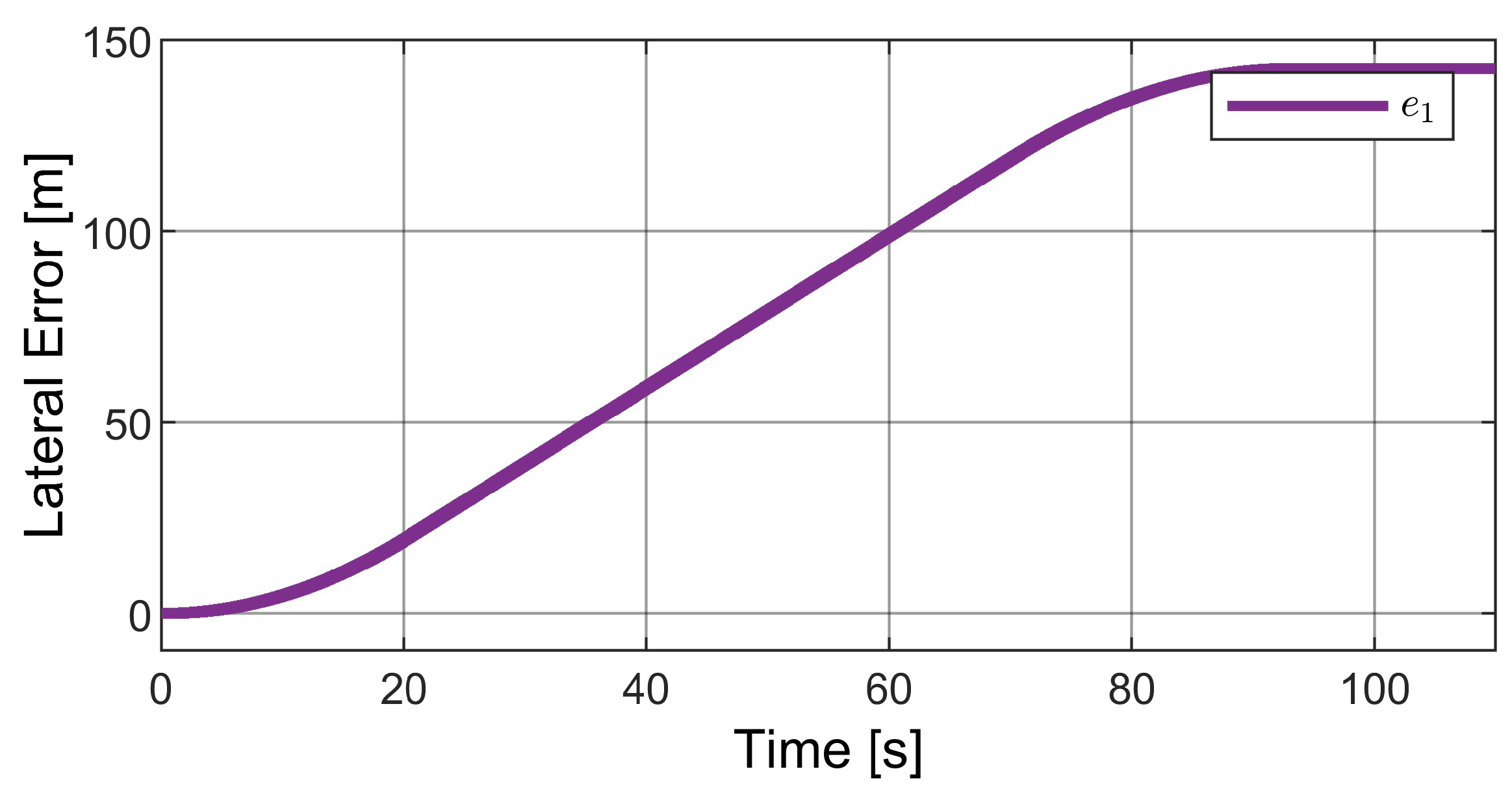
Adding the desired velocity profile to the suboptimal control gives the results presented in Figure 8 and Figure 9. Figure 8 shows the comparison between the velocity profile and the lateral velocity in the model. As observed, the control follows the velocity profile in the variable of e ˙ 1 , and the energy of the input control signal remains at a value less than 2 × 10 3 , see Figure 9. In this test, e 1 tracks the behavior of an integration of the velocity profile, Figure 10. During the first 20 s, where the velocity is increasing, the lateral displacement shows a curve. For the next 70 s, where the velocity is a constant value different from zero, the lateral displacement grows with the corresponding slope. During the time that the velocity is decreasing, the lateral displacement performs a curve in the opposite direction, and finally, when the velocity reaches zero again, the displacement becomes constant.

4. Discussion

The proposed suboptimal control solves the stabilization problem for the vehicle model without resorting to the small angle approximation and avoids solving the Bellman equation. The small angle approximation, while allowing the use of the linear model of the system, assumes that the argument of the arctan functions in the model is small.
Since the argument of the arctan functions depends on the velocity of the angle and the velocity of the lateral displacement, even with small angles in the entrance, we can have the case that the condition is not fulfilled, meaning that the argument is outside the linear behavior range. The obtained results indicate that the goal of having a control that does not rely on such assumption has been achieved.
Also, the simulation results showed that the proposed control system accomplished two important requirements. The first one is that the control easily stabilizes the whole system, and this is essential to make different control tasks with the vehicle. The second is that it keeps a moderate control signal, and this obeys the formulation as a suboptimal control; furthermore, the simulation demonstrates that the control signal generated is small in the task that implies a gradual change in the variables to track speed profiles. The simulations settings were standard for path planning of a vehicle. The results demonstrated that the suboptimal control successfully accomplishes these tasks and can be used to control the input angle δ to obtain a desired trajectory in y.
Summarizing, the main contribution of the present paper is a suboptimal control strategy for the vehicle based on the lateral position and the orientation errors with the following characteristics:
  • The proposed control algorithm uses the nonlinear dynamical model of the vehicle for the controller synthesis while the proposed controllers published in the literature are based on the linearized model of the vehicle.
  • The synthesis of the suboptimal control avoids the solution of the Bellman equation.

Author Contributions

Conceptualization, R.L. and S.S.; methodology, O.-J.S.-S.; software, L.R.; validation, L.R., O.-J.S.-S., S.S. and R.L.; formal analysis, O.-J.S.-S. and L.R.; investigation, L.R.; resources, R.L.; data curation, L.R.; writing—original draft preparation, L.R.; writing—review and editing, R.L., S.S. and O.-J.S.-S.; visualization, L.R.; supervision, O.-J.S.-S., S.S. and R.L.; project administration, S.S. All authors have read and agreed to the published version of the manuscript.

Funding

This research received no external funding.

Institutional Review Board Statement

Not applicable.

Informed Consent Statement

Not applicable.

Data Availability Statement

Not applicable.

Acknowledgments

This work was supported in part by the National Council of Humanities, Science and Technology (CONAHCYT) and the LAFMIA-CINVESTAV.

Conflicts of Interest

The authors declare no conflict of interest.

Abbreviations

The following abbreviations are used in this manuscript:
IMUInertial Measurement Unit
LQRLinear–quadratic regulator
MPCModel Predictive Control
NMPCNonlinear Model Predictive Control
c.g.center of gravity

References

  1. Jin, C.; Shao, L.; Lex, L.; Eichberger, A. Vehicle side slip angle observation with road friction adaptation. IFAC PapersOnLine 2017, 50, 3406–3411. [Google Scholar] [CrossRef]
  2. Xiong, L.; Xia, X.; Lu, Y.; Liu, W.; Gao, L.; Song, S.; Han, Y.; Yu, Z. IMU-based automated vehicle slip angle and attitude estimation aided by vehicle dynamics. Sensors 2019, 19, 1930. [Google Scholar] [CrossRef] [PubMed] [Green Version]
  3. Shao, K.; Zheng, J.; Deng, B.; Huang, K.; Zhao, H. Active steering control for vehicle rollover risk reduction based on slip angle estimation. IET Cyber-Syst. Robot. 2020, 2, 132–139. [Google Scholar] [CrossRef]
  4. Wang, Y.; Nguyen, B.M.; Fujimoto, H.; Hori, Y. Multirate estimation and control of body slip angle for electric vehicles based on onboard vision system. IEEE Trans. Ind. Electron. 2013, 61, 1133–1143. [Google Scholar] [CrossRef]
  5. Zhang, W. A robust lateral tracking control strategy for autonomous driving vehicles. Mech. Syst. Signal Process. 2021, 150, 107238. [Google Scholar] [CrossRef]
  6. Tagne, G.; Talj, R.; Charara, A. Higher-order sliding mode control for lateral dynamics of autonomous vehicles, with experimental validation. In Proceedings of the 2013 IEEE intelligent vehicles symposium (IV), Gold Coast, Australia, 23–26 June 2013. [Google Scholar]
  7. Fekih, A.; Seelem, S. Effective fault-tolerant control paradigm for path tracking in autonomous vehicles. Syst. Sci. Control Eng. 2015, 3, 177–188. [Google Scholar] [CrossRef]
  8. Wang, G.; Liu, L.; Meng, Y.; Gu, Q.; Bai, G. Integrated path tracking control of steering and differential braking based on tire force distribution. Int. J. Control Autom. Syst. 2022, 20, 536–550. [Google Scholar] [CrossRef]
  9. Moreno-Gonzalez, M.; Artuñedo, A.; Villagra, J.; Join, C.; Fliess, M. Speed-Adaptive Model-Free Path-Tracking Control for Autonomous Vehicles: Analysis and Design. Vehicles 2023, 5, 698–717. [Google Scholar] [CrossRef]
  10. Barari, A.; Saraygord Afshari, S.; Liang, X. Coordinated control for path-following of an autonomous four in-wheel motor drive electric vehicle. Proc. Inst. Mech. Eng. Part C 2022, 236, 6335–6346. [Google Scholar] [CrossRef] [PubMed]
  11. Chen, G.; Hua, M.; Zong, C.; Zhang, B.; Huang, Y. Comprehensive chassis control strategy of FWIC-EV based on sliding mode control. IET Intell. Transp. Syst. 2019, 13, 703–713. [Google Scholar] [CrossRef]
  12. Rajamani, R. Vehicle Dynamics and Control; Springer Science & Business Media: New York, NY, USA, 2012; pp. 15–46. [Google Scholar]
  13. Nguyen, A.T.; Rath, J.; Guerra, T.M.; Palhares, R.; Zhang, H. Robust set-invariance based fuzzy output tracking control for vehicle autonomous driving under uncertain lateral forces and steering constraints. IEEE Trans. Intell. Transp. Syst. 2020, 22, 5849–5860. [Google Scholar] [CrossRef]
  14. Taghavifar, H.; Rakheja, S. Path-tracking of autonomous vehicles using a novel adaptive robust exponential-like-sliding-mode fuzzy type-2 neural network controller. Mech. Syst. Signal Process. 2019, 130, 41–55. [Google Scholar] [CrossRef]
  15. Kirk, D.E. Optimal Control Theory: An Introduction; Courier Corporation: New York, NY, USA, 2004; pp. 67–86. [Google Scholar]
  16. Santos-Sánchez, O.; García, O.; Romero, H.; Salazar, S.; Lozano, R. Finite horizon nonlinear optimal control for a quadrotor: Experimental results. Optim. Control Appl. Methods 2021, 42, 54–80. [Google Scholar] [CrossRef]
  17. Ángeles-Rojas, D.; Santos-Sánchez, O.J.; Salazar, S.; Lozano, R. Finite Horizon Nonlinear Suboptimal Control for an Autonomous Soaring UAV. Math. Probl. Eng. 2022, 2022, 2214217. [Google Scholar] [CrossRef]
  18. Castillo, F.; López-Gutíerrez, R.; Santos-Sánchez, O.J.; Osorio, A.; Salazar, S.; Lozano, R. Finite Horizon Nonlinear Energy Optimizing Control in a Force Augmenting Hybrid Exoskeleton for the Elbow Joint. IEEE Trans. Control Syst. Technol. 2019, 28, 2681–2688. [Google Scholar] [CrossRef]
  19. Van den Bos, A. Appendix B: Vectors and Matrices. In Parameter Estimation for Scientists and Engineers; John Wiley & Sons, Ltd: Hoboken, NJ, USA, 2007. [Google Scholar] [CrossRef] [Green Version]
  20. Gilbert, G.T. Positive Definite Matrices and Sylvester’s Criterion. Am. Math. Mon. 1991, 98, 1. [Google Scholar] [CrossRef]
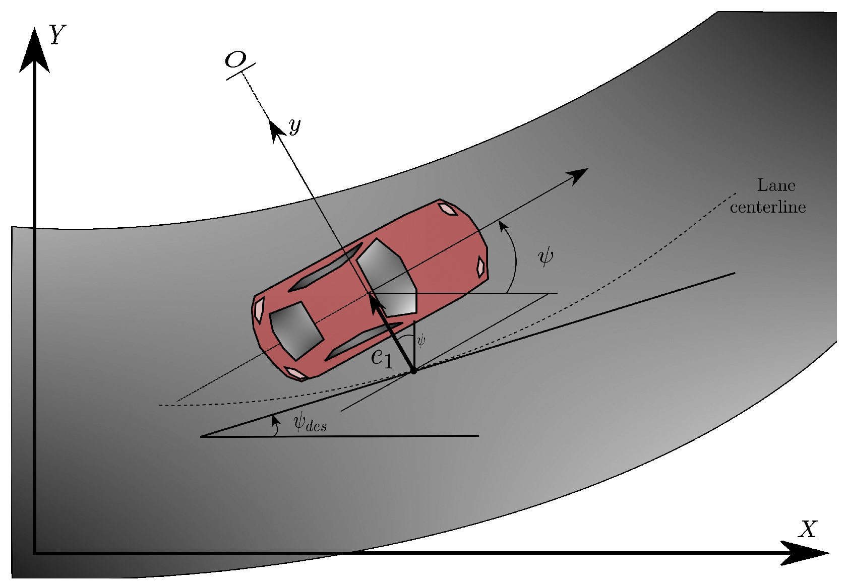
Figure 1. Lateral vehicle model considering the error in lateral position.
Vehicles 05 00053 g001
Figure 2. Block model implemented in Matlab Simulink for the lane-keeping test.
Vehicles 05 00053 g002
Figure 3. Block model implemented in Matlab Simulink for the tracking of a velocity profile.
Vehicles 05 00053 g003
Figure 4. Lane-keeping simulation with the suboptimal law applied, the objective is to reach e 1 = 0 m.
Vehicles 05 00053 g004
Figure 5. Control signal generated by the suboptimal control law in the lane-keeping simulation.
Vehicles 05 00053 g005
Figure 6. Orientation error when performing the lane-keeping simulation.
Vehicles 05 00053 g006
Figure 7. Predefined velocity profile for the simulation.
Vehicles 05 00053 g007
Figure 8. Result in simulation with the suboptimal control law for the variable e ˙ 1 .
Vehicles 05 00053 g008
Figure 9. Control signal generated by the suboptimal control law in the simulation with the predefined velocity profile.
Vehicles 05 00053 g009
Figure 10. Result in simulation for the variable e 1 , the suboptimal control law was used with the velocity profile.
Vehicles 05 00053 g010
Table 1. Model variables.
VariablesDescription
e 1 Distance between the center of gravity (c.g.) and the center of the lane
e 2 Orientation error between the orientation of the vehicle and the road orientation
δ Front wheel steering angle
V x Longitudinal velocity of the c.g. of the vehicle
ψ ˙ d e s Rate of change of the desired orientation of the vehicle
C α f Individual cornering stiffness (front tires)
C α r Individual cornering stiffness (rear tires)
f Distance of front steer axle from the c.g.
r Distance of rear steer axle from the c.g.
Table 2. Parameters required for the simulation 1.
ParameterValueUnit
m1573Kg
I z 2873Kgm 2
f 1.1m
r 1.58m
C α f 80,000N/rad
C α r 80,000N/rad
1 These parameters represent a passenger sedan [12].
Disclaimer/Publisher’s Note: The statements, opinions and data contained in all publications are solely those of the individual author(s) and contributor(s) and not of MDPI and/or the editor(s). MDPI and/or the editor(s) disclaim responsibility for any injury to people or property resulting from any ideas, methods, instructions or products referred to in the content.