Mix Controller Design for Active Suspension of Trucks Integrated with Online Estimation of Vehicle Mass

Abstract

Active suspension can improve vehicle vibrations caused by road excitation. For trucks, the vehicle mass change is usually large, and changes in vehicle mass will affect the control performance of the active suspension. In order to solve the problem of active suspension control performance decreasing due to large changes in vehicle mass, this paper proposes an active suspension control method integrating online mass estimation. This control method is designed based on the mass estimation algorithm of the recursive least squares method with a forgetting factor (FFRLS) and the Linear Quadratic Regulator (LQR) algorithm. A set of feedback control matrices $K$ is obtained according to different vehicle masses. Then, the mass estimation algorithm can estimate the actual vehicle mass in real-time during the vehicle acceleration process. According to the mass estimation value, a corresponding feedback control matrix $K$ is selected from the control matrix set, and $K$ is used as the actual control gain matrix of the current active suspension. With specific simulation cases, the vehicle vibration response is studied by the numerical simulation method. The results of the simulation process have shown that when the vehicle mass changes largely, the suspension dynamic deflection and tire dynamic deformation are significantly reduced while keeping a good vehicle body attitude control effect by using an active suspension controller integrated with online mass estimation. In the random road simulation, suspension dynamic deflection is reduced by 3.26%, and tire dynamic deformation is reduced by 5.91% compared with the original active suspension controller. In the road bump simulation, suspension dynamic deflection and tire dynamic deformation are also significantly reduced. As a consequence, the stability and comfort of the vehicle have been greatly enhanced.

1. Introduction

With the help of advanced sensors, controllers, and actuators, the active suspension can sense the vehicle’s motion state and road surface condition in real-time [1], and actively adjust the actuator force, which can significantly improve the vehicle’s driving performance under various working conditions.

In the field of modern logistics and transportation, the active suspension system control method on trucks has been a research hotspot for many years [2,3]. The suspension control system typically utilizes fixed vehicle parameters; however, the truck’s mass can change significantly due to varying loads. If these fixed vehicle parameters are still used to control the truck suspension, it will significantly impact the truck’s stability and maneuverability [4,5]. Therefore, it is necessary to integrate real-time online mass estimation into the design of suspension controllers to ensure the trucks’ active suspension system control performance under various load conditions.

For vehicle mass estimation, this is typically performed using a longitudinal vehicle dynamic model. Early studies mostly used simplified longitudinal dynamics models integrated with least squares (LS) or recursive least squares (RLS) for vehicle status estimation [6,7]. Such methods reduce computational complexity by simplifying the model framework, but have limited ability to deal with nonlinear characteristics and parameter coupling problems.

To solve the estimation accuracy problem in nonlinear systems, some scholars realized vehicle status estimation by constructing a nonlinear longitudinal dynamics model and improved real-time performance through the data discretization method; four different states were set to simulate real-time working conditions, respectively [8]. Some other scholars have accomplished online vehicle mass estimation by constructing a nonlinear longitudinal model integrated with a state observer [9]. This method improved the vehicle speed tracking accuracy and control robustness under complex working conditions.

To address the problem of utilizing multi-source data under complex working conditions, some scholars have improved mass estimation accuracy by separating the coupling relationship between mass and slope using the RLS algorithm with a forgetting factor, based on the longitudinal dynamic model [10]. Other scholars have proposed an estimation framework based on a combination of NPF and CKF for HDV characteristics and real transportation scenarios. A low-pass filter and a KF-based data fusion method are added to the estimation framework [11]. Others have developed an unknown input observer to estimate the augmented system states, while a linear matrix inequality and an estimated states correction method are introduced to further attenuate the effects of residual disturbances and thus guarantee the accuracy of the estimation [12]. These methods were used to enhance estimation accuracy under complex operating conditions by extending model dimensions or integrating data.

The suspension system is a key component of an automobile, and its effective control can significantly improve driving stability and ride comfort [13]. Today, there are numerous suspension control methods, including skyhook damping control [14], fuzzy control [15,16], optimal control [17,18], and deep learning control [19]. Within optimal control algorithms, the Linear Quadratic Regulator (LQR) can perform multi-objective optimization of the controlled system [20]. Multi-objective optimization can significantly enhance the vibration characteristics of automotive suspension systems [21,22,23]. Good vibration characteristics can effectively suppress the bumps generated by road roughness [24], which is an important factor in ensuring vehicle stability, reducing body shaking and impact, and is of great significance in improving the overall performance and safety of the vehicle [25]. The application of LQR to suspension systems can help better balance vehicle driving stability and ride comfort [26].

To achieve better control performance of the active suspension system, some scholars have developed an effective control algorithm by designing an optimization-sliding mode control (OSMC) algorithm [27], which is based on nonlinear control theory and Lyapunov stability theory. In addition to the above study, the adaptive fuzzy sliding mode proportional–integral differentiation (AFSPIDF) algorithm has been proposed, which integrates multiple algorithms [28], providing a new idea for controlling an active suspension system. To address the problem that certain vehicle states cannot be measured and that external disturbances can impact vertical dynamics, some scholars have proposed a solution to overcome the problem of fault-tolerant event-triggered control, which enhances vehicle performance and comfort by reducing body accelerations over time for the nonlinear model [29]. All these scholars have made considerable contributions to automobile active suspension control, but regarding the truck suspension control system, the truck mass change after loading has a certain effect on the suspension control performance, and this problem should not be ignored.

Motivated by the reasons above, this paper proposes a suspension control system model that integrates vehicle mass estimation and fully considers the impact of mass change on suspension control performance. The specific works are shown below:

(1)

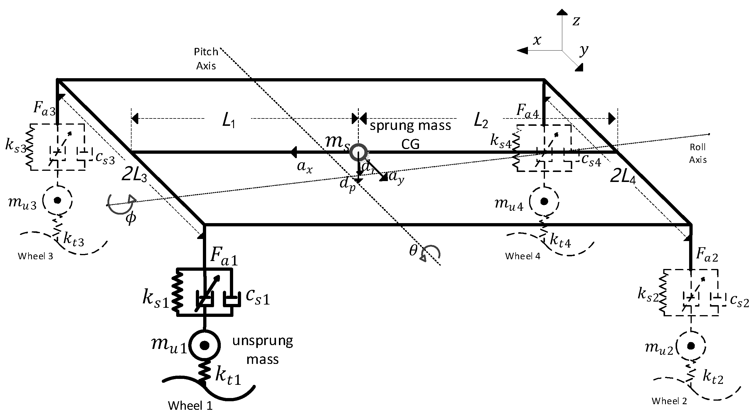
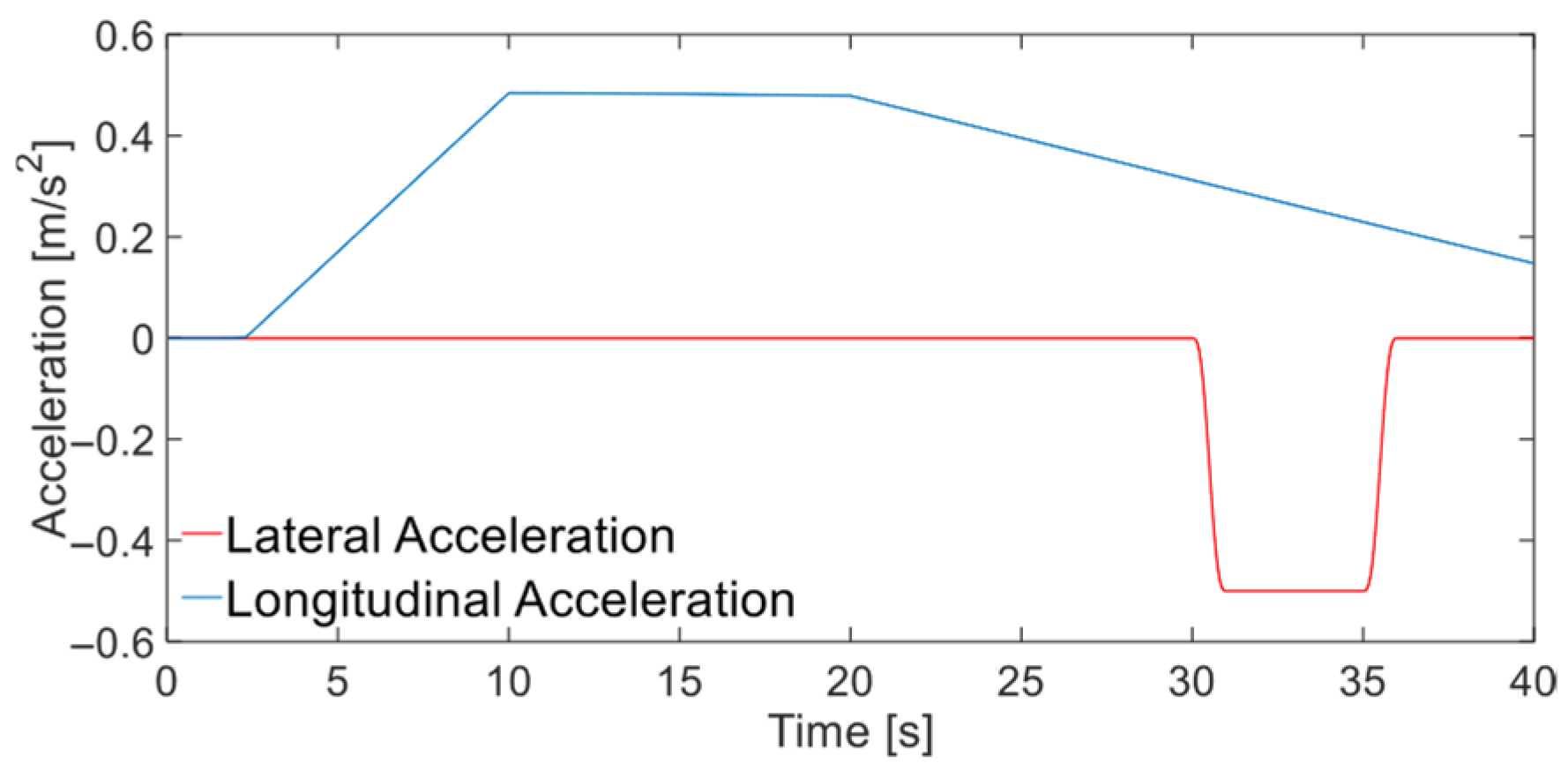
A seven-degree-of-freedom vehicle active suspension model considering road excitation, lateral, and longitudinal acceleration is established.

(2)

A recursive least squares algorithm with a forgetting factor for vehicle mass estimation is established.

(3)

An active suspension mix controller, LQR controller with integrated vehicle mass estimation, is proposed.

To verify the control strategy’s effectiveness, the dynamic response and body attitude control are designed and analyzed through numerical simulation. The body vertical acceleration, body pitch angle, body roll angle, suspension dynamic deflection, and tire dynamic deformation are used as evaluation metrics. The simulation results are compared with the uncontrolled passive suspension and the LQR controller without integrated mass estimation (original controller) in the time and frequency domains.

2. Multi-Degree-of-Freedom Coupling Dynamics Model of the Vehicle

To consider the lateral, longitudinal, and vertical characteristics, a vehicle mass coupling dynamics model with multiple degrees of freedom is established, which includes a total of seven degrees of freedom, including the vertical, pitch, and lateral movements of the body and the vertical movement of the unsprung mass, as shown in Figure 1.

All parameters in Figure 1 are defined as shown in

Table 1. Vehicle parameters.

Parameters	Symbol	Parameters	Symbol
Sprung mass	$m_s$	Distance from the mass center to the front axes	$L_1$
Vertical displacement of the sprung mass center	$z$	Distance from the mass center to the rear axes	$L_2$
Total suspension forces of the $i$-th wheel	$F_{si}$	Distance from the mass center to the front half shaft base	$L_3$
Suspension stiffness of the $i$-th wheel	$k_{si}$	Distance from the mass center to the rear half shaft base	$L_4$
Suspension damping of the $i$-th wheel	$c_{si}$	Longitudinal accelerations of the mass center	$a_x$
Ideal damping force of the $i$-th wheel	$F_{ai}$	Lateral accelerations of the mass center	$a_y$
Unsprung mass vertical displacement of the $i$-th wheel	$z_{ui}$	Distance from the sprung mass center to the pitch axes	$d_r$
Sprung mass vertical displacement of the $i$-th wheel	$z_{si}$	Distance from the sprung mass center to the roll axes	$d_p$
Acceleration of gravity	g	Roll angles of the sprung mass	$\varphi$
Lateral moment of inertia of the sprung mass	$I_x$	Pitch angles of the sprung mass	$\theta$
Pitch moment of inertia of the sprung mass	$I_y$	Unsprung mass of the $i$-th wheel	$m_{ui}$
Road input of the $i$-th wheel	$z_{gi}$	Tire stiffness of the $i$-th wheel	$k_{ti}$

Note $i=1,2,3,4$, are the left front wheel, left rear wheel, right front wheel, and right rear wheel, respectively.

.

According to Newton’s second law, the vertical vibration equation at the center of mass is

$$m_s\ddot{z}=\sum _{i=1}^4 F_{si}$$

(1)

The total suspension forces expressed by $F_{si}$ is the sum of the elastic force, the damping force, and the suspension actuator force, which can be expressed as

$$F_{si}=k_{si}\left(z_{ui}-z_{si}\right)+c_{si}\left({\dot{z}}_{ui}-{\dot{z}}_{si}\right)+F_{ai}$$

(2)

Under the effect of inertial acceleration, the equations of motion for the rolling and pitching of the sprung mass can be expressed, respectively, as

$$I_x\ddot{\varphi }=(F_{s1}-F_{s3})L_3+(F_{s2}-F_{s4})L_4+m_s{a}_y{d}_r+m_{s}g{d}_r\varphi$$

(3)

$$I_y\ddot{\theta }=\left(F_{s2}+F_{s4}\right)L_2-\left(F_{s1}+F_{s3}\right)L_1+m_s{a}_x{d}_p+m_{s}g{d}_p\theta$$

(4)

The vibration equation for an unsprung mass is

$$m_{ui}{\ddot{z}}_{ui}=k_{ti}(z_{gi}-z_{ui})-F_{si}$$

(5)

When the roll angle and pitch angle are varied in a very small range, the displacements of the $i$-th wheel’s sprung mass are, respectively,

$$z_{si}=\left\{\begin{array}{c}z-L_1\theta +L_3\varphi \hfill \\ z+L_2\theta +L_4\varphi \hfill \\ z-L_1\theta -L_3\varphi \hfill \\ z+L_2\theta -L_4\varphi \hfill \end{array}\right.$$

(6)

Define

$$M_s=diag\left(m_s,I_s,I_s\right),$$

$$C_s=diag(c_{s1},c_{s2},c_{s3},c_{s4}),$$

$$K_s=diag\left(k_{s1},k_{s2},k_{s3},k_{s4}\right),$$

$${ K}_t=diag\left(k_{t1},k_{t2},k_{t3},k_{t4}\right),$$

$${ F}_a=[F_{a1},F_{a2},F_{a3},F_{a4}{]}^T,$$

$$Z_s=[z_0,\varphi ,\theta {]}^T,$$

$$Z_U=[z_{u1},z_{u2},z_{u3},z_{u4}{]}^T,$$

$${ Z}_G=[z_{g1},z_{g2},z_{g3},z_{g4}{]}^T,$$

$$L_{\mathrm{m}1}=\left[\begin{array}{cc}0& 0\\ m_s{d}_r& 0\\ 0& m_s{d}_p\end{array}\right],$$

$${ L}_{m2}=\left[\begin{array}{ccc}0& 0& 0\\ 0& m_{s}g{d}_r& 0\\ 0& 0& m_{s}g{d}_p\end{array}\right],$$

$$L=\left[\begin{array}{cccc}1& 1& 1& 1\\ L_3& L_4& -L_3& -L_4\\ -L_1& L_2& -L_1& L_2\end{array}\right].$$

The vibration equations for the sprung mass and unsprung mass can be simplified to matrix form

$$M_S{\ddot{Z}}_S=L{K}_S(Z_U-L^T{Z}_S)+L{C}_S({\dot{Z}}_U-L^T{\dot{Z}}_S)+L{F}_a+L_{m1}{Z}_a+L_{m2}{Z}_S$$

(7)

$$M_U{\ddot{Z}}_U=K_t(Z_G+Z_U)-K_S(Z_U-{L^{T}Z}_S)-C_S({\dot{Z}}_U-{L^T\dot{Z}}_S)-F_a$$

(8)

To design the controller, the above equation is expressed in matrix form as a state equation of the form

$$\left\{\begin{array}{c}\dot{X}=AX+BU+GW\hfill \\ Y=CX+DU+HW\hfill \end{array}\right.$$

(9)

state variables

$$X=[Z_S Z_S Z_U-L^T{Z}_s Z_G-Z_U Z_U{]}^T$$

output variable

$$Y=[\begin{array}{cccc}{\ddot{Z}}_S& Z_S& Z_U-L^T{Z}_S& Z_G-Z_U\end{array}{]}^T$$

actuator force input

$$U=F_a$$

the vehicle’s perturbation vector is

$$W=Z_G$$

the vehicle’s system matrixes are

$$A={\left[\begin{array}{ccccc}{0}_{3\times 3}& I_{3\times 3}& 0_{3\times 4}& 0_{3\times 4}& 0_{3\times 4}\\ M_S^{-1}{L}_{m2}& -M_S^{-1}L{C}_S{L}^T& M_S^{-1}L{K}_S& 0_{3\times 4}& M_S^{-1}L{C}_S\\ 0_{4\times 3}& -L^T& 0_{4\times 4}& 0_{4\times 4}& I_{4\times 4}\\ 0_{4\times 3}& 0_{4\times 3}& 0_{4\times 4}& 0_{4\times 4}& -I_{4\times 4}\\ 0_{4\times 3}& M_U^{-1}{C}_S{L}^T& -M_U^{-1}{K}_S& M_U^{-1}{K}_t& -M_U^{-1}{C}_S\end{array}\right]}_{18\times 18},$$

$$B={\left[\begin{array}{c}{0}_{3\times 4}\\ M_S^{-1}L\\ 0_{4\times 4}\\ 0_{4\times 4}\\ -M_U^{-1}\end{array}\right]}_{18\times 4} ,G={\left[\begin{array}{cc}{0}_{3\times 2}& 0_{3\times 4}\\ M_S^{-1}{L}_{\mathrm{b}\mathrm{u}\mathrm{l}}& 0_{3\times 4}\\ 0_{4\times 2}& 0_{4\times 4}\\ 0_{4\times 2}& I_{4\times 4}\\ 0_{4\times 2}& 0_{4\times 4}\end{array}\right]}_{18\times 6},$$

$$C={\left[\begin{array}{ccccc}{M}_S^{-1}{L}_{\mathrm{m}2}& -M_S^{-1}L{C}_S{L}^T& M_S^{-1}L{K}_S& 0_{3\times 4}& M_S^{-1}L{C}_S\\ I_{3\times 3}& 0_{3\times 3}& 0_{3\times 4}& 0_{3\times 4}& 0_{3\times 4}\\ 0_{4\times 3}& 0_{4\times 3}& I_{4\times 4}& 0_{4\times 4}& 0_{4\times 4}\\ 0_{4\times 3}& 0_{4\times 3}& 0_{4\times 4}& I_{4\times 4}& 0_{4\times 4}\end{array}\right]}_{14\times 18},$$

$$D={\left[\begin{array}{c}{M}_s^{-1}L\\ 0_{3\times 4}\\ 0_{4\times 4}\\ 0_{4\times 4}\end{array}\right]}_{14\times 4} ,H={\left[\begin{array}{cc}{M}_S^{-1}{L}_{\mathrm{m}\mathrm{i}}& 0_{3\times 4}\\ 0_{3\times 2}& 0_{3\times 4}\\ 0_{4\times 2}& 0_{4\times 4}\\ 0_{4\times 2}& 0_{4\times 4}\end{array}\right]}_{14\times 6}.$$

where $I_{m\times n}$ is the identity matrix.

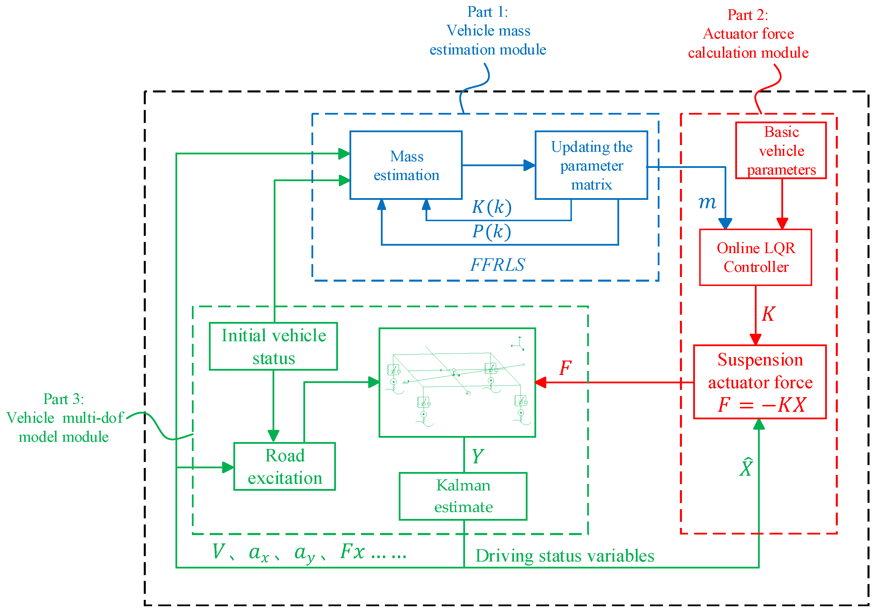
3. Mix Control System Architecture for Active Suspension Integrated with Mass Estimation

For trucks, the load mass significantly affects the active suspension control performance, and vehicle mass remains relatively stable and unchanged throughout the driving process [30]. The LQR controller architecture is shown in Figure 2. The traditional LQR algorithm cannot make relative adjustments to changes in vehicle mass, so it is necessary to integrate the mass estimation algorithm. The algorithm of recursive least squares with forgetting factor (FFRLS) is used to estimate the vehicle mass, and the mix controller adjusts the active suspension control based on the estimated vehicle mass, achieving a more optimal effect on the vehicle suspension control performance. The architecture of the vehicle control strategy is shown in Figure 3.

The architecture for the mix controller is divided into three parts: part 1 is the vehicle mass estimation module, part 2 is the actuator force calculation module, and part 3 is the vehicle multi-degree-of-freedom (multi-dof) model module. Part 1 estimates the vehicle mass by the FFRLS, and outputs the vehicle mass; part 2 recognizes the vehicle mass and real-time state variables by the online LQR controller, and calculates the optimal solution of the actuator force, and part 3 accepts the actuator force output by the online LQR controller, and transmits the real-time driving state variables to part 1 and part 2.

4. Design of Active Suspension Mix Controller

4.1. Module for Recursive Least Squares with Forgetting Factor for Vehicle Mass Estimation

4.1.1. Vehicle Mass Estimation Model

According to Newton’s second law, the longitudinal motion equation of the vehicle is as follows

$$m\dot{v}=F_X-F_f-F_w-F_i$$

(10)

expanding the equation gives

$$m\dot{\nu }={\displaystyle \frac{T_{tq}{i}_g{i}_0{\eta }_T}{r}}-{\displaystyle \frac{1}{2}}\rho C_{d}A{v}^2-mg\mathrm{s}\mathrm{i}\mathrm{n} \alpha -mgf\cos \alpha$$

(11)

where $F_x$ is the longitudinal driving force, $F_f$ is the rolling resistance, $F_w$ is the air resistance, $F_i$ is the ramp resistance, $m$ is the mass of the vehicle, $v$ is the longitudinal speed of the vehicle, $T_{tq}$ is the actual torque input from the engine to the transmission, $i_g$ is the transmission ratio, $i_0$ is the main gearbox ratio, ${\eta }_T$ is the mechanical efficiency of the driveline, $r$ is the rolling radius of the wheels, $\rho$ is the air density, $C_d$ is the wind resistance coefficient, $A$ is the windward surface area, $\alpha$ is the roadway gradient, $f$ is the road roll resistance coefficient.

The equation is transformed as follows:

$${\displaystyle \frac{T_{tq}{i}_g{i}_0{\eta }_T}{r}}-{\displaystyle \frac{1}{2}}\rho C_{d}A{v}^2=m(\dot{v}+g\mathrm{s}\mathrm{i}\mathrm{n} \alpha +gf\mathrm{c}\mathrm{o}\mathrm{s} \alpha )$$

(12)

4.1.2. Recursive Least Squares Algorithm with Forgetting Factor

Recursive least squares (RLS) utilizes the criterion of least squares (LS), and its principle is to minimize the model estimation error by using the exponential weighted error sum of squares. The RLS algorithm has good convergence and tracking ability, and its computational volume is small [31]. The forgetting factor $\lambda$ can dilute or enhance the influence of historical data on the current estimation and improve algorithm adaptability [32]. The effect of $\lambda$ on historical data is shown in

Table 2. Effect of forgetting factors on historical data.

The Range of $\mathit{\lambda }$	Effect on Historical Data
0 < $\lambda$ <1	diluted
$\lambda$ = 1	unaffected
$\lambda$ > 1	enhanced

.

In this paper, we set the value of the forgetting factor to $\lambda$ = 0.95.

According to the longitudinal vehicle dynamic model, the mass estimation input-output recursive equation of recursive least squares with forgetting factor (FFRLS) is established

$$y(k)=h(k{)}^T\widehat{\theta }+e(k)$$

(13)

where $h\left(k\right)$ is the input, which is the measurable data vector; $y\left(k\right)$ is the output of the system; $\widehat{\theta }$ is the parameter to be estimated, and the parameter in this paper is vehicle mass $m$.

From the longitudinal dynamic equation, the below can be obtained:

$$y={\displaystyle \frac{T_{tq}{i}_g{i}_0{\eta }_T}{r}}-{\displaystyle \frac{1}{2}}\rho C_{d}A{v}^2$$

(14)

$$h=\dot{\nu }+g\mathrm{s}\mathrm{i}\mathrm{n} \alpha +gf\mathrm{c}\mathrm{o}\mathrm{s} \alpha$$

(15)

The steps of FFRLS are as follows:

(1)

Solve for parameter identification gain

$$K(k)={\displaystyle \frac{P(k-1)h\left(k\right)}{\lambda +h\left(k{)}^{T}P\right(k-1\left)h\right(k)}}$$

(16)

(2)

Update parameter identification

$$\widehat{\theta }(k)=\widehat{\theta }(k-1)+K(k)\left[y(k)-h{(k)}^T\widehat{\theta }(k-1)\right]$$

(17)

(3)

Update recognition error

$$P(k)={\displaystyle \frac{1}{\lambda }}\left[I-K(k)h{\left(k\right)}^T\right]P(k-1)$$

(18)

where $K\left(k\right)$ is the parameter identification gain at moment $k$; $P\left(k\right)$ is the covariance matrix at moment $k$; $I$ is the identity matrix.

The estimated vehicle mass $m$, sprung mass $m_s$, and unsprung mass $m_{ui}$ are related as

$$m=\sum _{i=1}^4 m_{ui}+m_s$$

(19)

where the unsprung mass $m_{ui}$ is a fixed preset value, and the sprung mass $m_s$ can be calculated by the mass estimator after estimating the vehicle mass $m$.

4.2. Module for LQR-Based Actuator Force Calculation

The Linear Quadratic Regulator (LQR) controller is a full-state feedback controller that minimizes error by means of an objective function and a suitable gain matrix, allowing the system to achieve better performance. The LQR cost function is chosen as follows

$$J={\int }_0^{\mathrm{\infty }} [Y^{T}QY+U^{T}RU]dt$$

(20)

where the input and output weight matrices are, respectively, as follows

$$Q=diag(q_1,q_2,q_3,q_4\dots \dots q_{14})$$

(21)

$$R=diag(r_1,r_2,r_3,r_4)$$

(22)

In the weight matrix, $q_1$~$q_{14}$ are the state variable weight coefficients, and $r_1$~$r_4$ are the actuator force weight coefficients. $q$ and $r$ reflect the relative importance of outputs and inputs. Empirical formulas are generally used to select the values of $q$ and $r$, and their values in this article are shown in

Table 3. Weight coefficient parameters.

	$q_1$	$q_1$	$q_1$	$q_1$	$q_1$	$q_1$	$q_{7-10}$	$q_{11-14}$	$r_1$~$r_4$
optimization solution	104.21	10−2.87	10−2.59	10+5.41	108.81	107.21	104.87	108.49	10−1.27

.

By modifying the above equation, the standard form of LQR cost function can be obtained as

$$J={\int }_0^{\mathrm{\infty }} {\left[\begin{array}{c}X\\ U\end{array}\right]}^T\left[\begin{array}{cc}E& N\\ N^T& F\end{array}\right]\left[\begin{array}{c}X\\ U\end{array}\right]dt$$

(23)

included among these

$$\left\{\begin{array}{c}E=C^{T}QC\hfill \\ F=D^{T}QD+R\hfill \\ N=C^{T}QD\hfill \end{array}\right.$$

(24)

By solving the Riccati equation in the following form

$$A^{T}P+PA-(PB+N)F^{-1}(B^{T}P+N^T)+E=0$$

(25)

obtain the positive definite solution matrix $P$. The feedback gain matrix of the controller is

$$K=F^{-1}(B^{T}P+N^T)$$

(26)

The following condition also should hold

$$\left[\begin{array}{cc}E& N\\ N^T& F\end{array}\right]>0$$

To obtain the system status, a Kalman filter is used to estimate the system status $\widehat{X}$

$$\dot{\widehat{X}}=A\widehat{X}+BU+R(Y-C\widehat{X}-DU)$$

(27)

where, by solving another Riccati equation,

$$\overline{F}=F_n+H{N}_n+N_n^T{H}^T+H{E_{n}H}^T$$

(28)

$$\overline{N}=V(E_n{H}^T+N_n)$$

(29)

The gain matrix of the Kalman filter can be obtained

$$R=({SC}^T+\overline{N})F^{-1}$$

(30)

where

$$\left\{\begin{array}{c}{E}_n=E(W{W}^T)\hfill \\ F_n=E(u{u}^T)\hfill \\ N_n=E(W{u}^T)\hfill \end{array}\right.$$

(31)

where $u$ is the nominal measurement noise in the Kalman estimation.

Finally, the actuator force is obtained as

$$U=-K\widehat{X}$$

(32)

4.3. Mix Control Logic

First, the mix LQR controller accepts the vehicle estimation mass by FFRLS, and calculates the vehicle’s system matrices $A, B,C,D,G,H$ in real-time based on the estimated mass and the preset basic parameters. The system matrices are input into the LQR controller to compute the controller’s feedback gain matrix $K$ in real-time, and then the mix LQR controller computes the optimal actuator force $U,$ as shown in Equation (32).

To obtain the feedback gain $K$ of the LQR controller, the Riccati equation needs to be solved, which requires high arithmetic power, making it difficult to be deployed in real-time in vehicle controllers. Therefore, the mass intervals are pre-divided according to the variation range of the vehicle mass, and all the feedback matrices are solved offline and summarized as a table of state feedback matrices. In real-time operation, according to the mass estimation result, the feedback matrix close to the estimated mass is selected from the table as the active suspension control gain. In this paper, the mass range 1200–2400 kg is divided into several intervals with 20 kg intervals each.

To prevent the estimated mass change from causing the feedback gain matrix $K$ to change too frequently, a mass change suppression module is used. This module introduces the absolute percentage error (APE) metric of the estimated mass to determine whether the $m_{out}$ is updated or not

$$APE=\left|m_{out}-m_{new}\right|/m_{out}$$

(33)

$$m_{out}=\left\{\begin{array}{c}{m}_{out}, APE\le \rho ;\hfill \\ m_{new}, else.\hfill \end{array}\right.$$

(34)

where $m_{out}$ is the current vehicle mass used to calculate the feedback gain matrix $K$, $m_{new}$ is the estimated vehicle mass at the current moment, and $\rho$ is the threshold value. The value of $m_{out}$ remains unchanged when $APE\le \rho$; conversely, $m_{out}$ is updated.

5. Comparative Simulation Analysis

The vehicle system is subjected to complex maneuvering excitation and random road excitation in practice. To conform to the practical vehicle operating condition, the combined working condition that can respond to the lateral, longitudinal, and vertical motions of the system is designed in this paper. The combined working conditions can stimulate the coupling of vehicle motions in each degree of freedom, such as the vertical vibration of the unsprung mass and the sprung mass, and the coupling motion of body pitch and roll.

To verify the design strategy effectiveness, the passive suspension, original controller, and mix controller are analyzed by numerical simulation using random road excitation and a road bump, respectively. The random road excitation adopts the filtered white noise time-domain road input model [33], which is as follows:

$${\dot{z}}_{gi}(t)=-2\pi f_0{z}_{gi}(t)+2\pi \sqrt{G_0\nu }{w}_i(t)$$

(35)

where the lower cut-off frequency of $f_0,w_i(t)$ is the uniformly distributed white noise of the $i$-th wheel, and $G_0$ is the road roughness coefficient.

In this paper, the left and right wheels are coherent, while the front and rear wheels exhibit a lag in response to road excitation. The relationship between the coherence and lag of the road excitation of each wheel is as described in the reference [34]. We use class B pavement as the random road input, the roughness coefficient of class B pavement is $G_0=0.000064$, and the lower cut-off frequency is taken as $f_0=0.01$.

5.1. Vehicle Simulation Parameter Selection

The values of the vehicle parameter used for simulation are shown in

Table 4. Vehicle parameter values.

Parameters	Symbol	Value	Unit
Nominal vehicle mass	$\overline{m}$	1200	kg
Vehicle actual mass	$m$	2000	kg
Air density	$\rho$	1.18	kg·m−3
Windward area	$A$	1.6	m2
Coefficient of air resistance	$C_d$	0.3
Coefficient of rolling friction	$f$	0.015
Acceleration of gravity	g	9.81	m·s−2
Centroid to front axes distance	$L_1$	1.178	m
Centroid to rear axes distance	$L_2$	1.464	m
Centroid to roll axes distance	$d_r$	0.256	m
Centroid to pitch axes distance	$d_p$	0.104	m
Front half shaft base	$L_3$	0.729	m
Rear half shaft base	$L_4$	0.7275	m
Unsprung mass at front wheels	$m_{u1},m_{u3}$	40.5	kg
Unsprung mass at rear wheels	$m_{u2},m_{u4}$	45.4	kg
Roll inertia	$I_x$	522	kg·m2
Pitch inertia	$I_y$	2131	kg·m2
Suspension stiffness	$k_{si}$	20,000	N·m−1
Wheel stiffness	$k_{ti}$	200,000	N·m−1

.

5.2. Dynamic Response and Body Attitude Analysis Integrated with Online Estimation of Vehicle Mass

First, the validity of the vehicle mass estimation algorithm is verified, and then the effects of vehicle dynamics response and body attitude control are compared between passive suspension, LQR controller without integrated vehicle mass estimation (original controller), and LQR controller with integrated vehicle mass estimation (mix controller).

The vehicle longitudinal velocity and longitudinal acceleration are shown in Figure 4 and Figure 5, respectively.

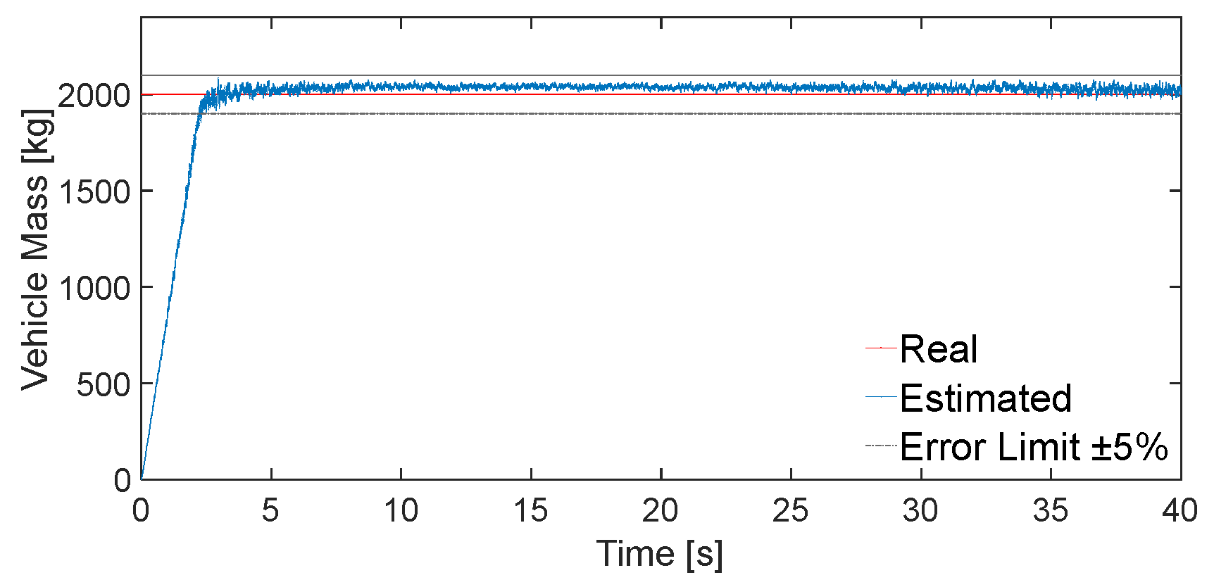
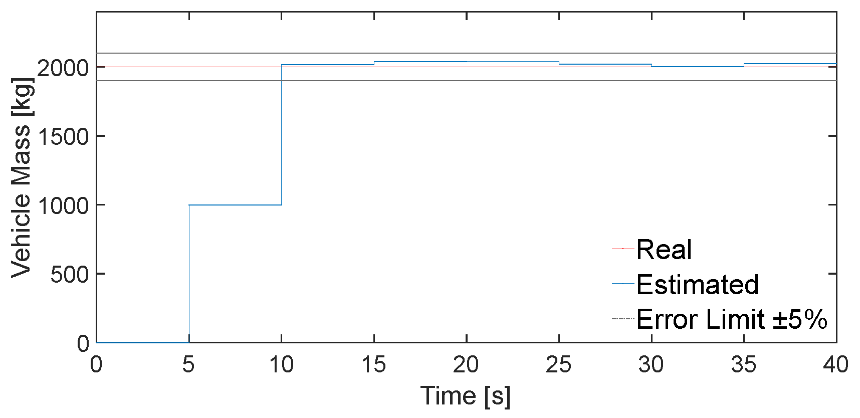
5.2.1. Vehicle Mass Estimation Simulation Analysis

The vehicle mass estimation result is shown in Figure 6.

As shown in Figure 6, the mass estimation algorithm designed in this paper can effectively estimate the vehicle mass within a short time, reducing the error to within 5%. To enable the mass estimation value to respond more effectively in the mix controller, the mass estimation value is averaged every 5 s, as shown in Figure 7.

To more accurately describe the error, this paper further adopts evaluation indices to reflect the error result. The selection of evaluation indices directly affects the judgment of control performance, and the commonly used evaluation indices are error integration indices. These indices mainly include ISE and IAE, which are defined in

Table 5. Error integrator index.

Integrator Index	Characteristic
$\mathrm{ISE}={\int }_0^t{e}^{2}dt$	Fast response, large overshoot, poor stability.
$\mathrm{IAE}={\int }_0^t\left|e\right|dt$	Focuses on late response error, less consideration of pre-response errors.

.

The 10 s after stabilization of the mean-processed mass estimation are analyzed, and the results are shown in

Table 6. Error results.

Index	ISE	IAE
Vehicle mass (t)	0.0096	0.28

. It can be seen that the mass estimation error is small.

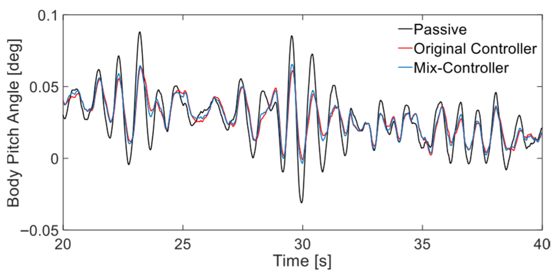
5.2.2. Vehicle Dynamic Response and Body Attitude Analysis

To study the effect of load change on active suspension control performance, this paper adopts a variable load condition, where the load is changed from 1200 kg to 2000 kg. The system is then subjected to lateral and longitudinal loading, and the vehicle’s corresponding lateral and longitudinal accelerations are shown in Figure 8.

Since the mass estimation takes some time to converge, the dynamic response and body attitude analysis are performed below for 20–40 s.

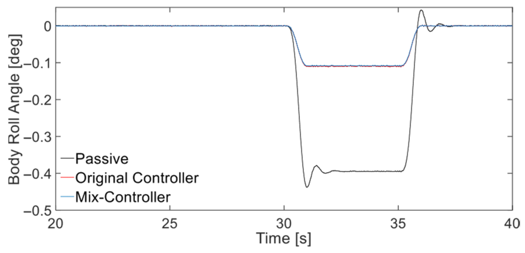
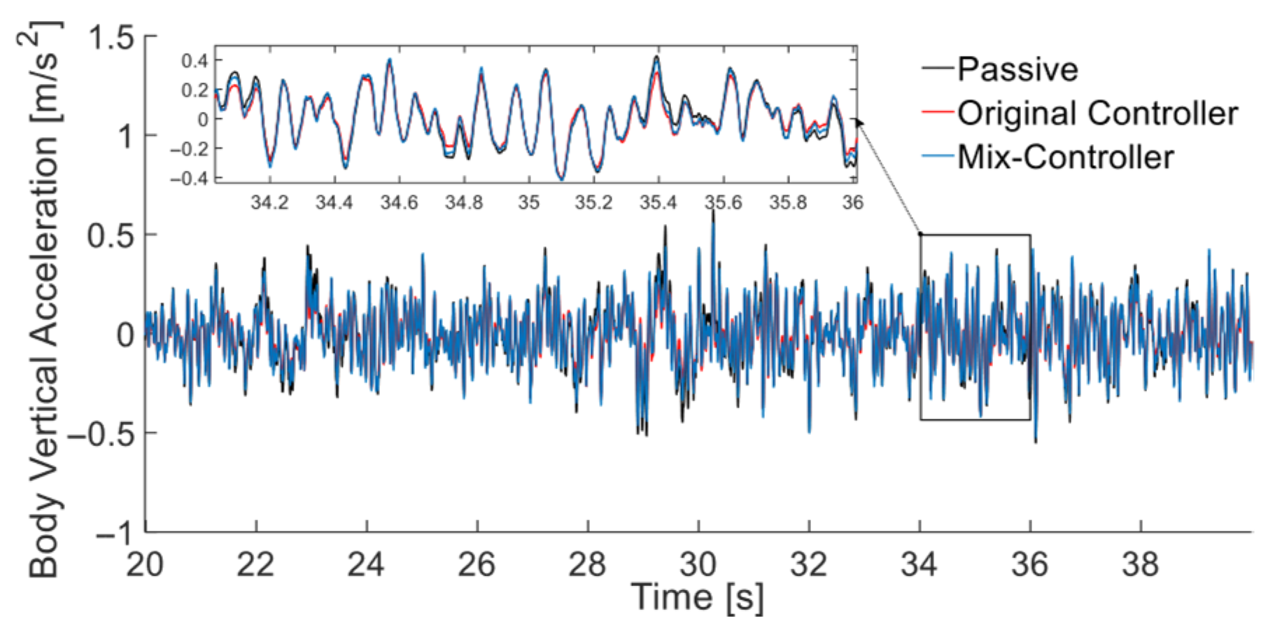
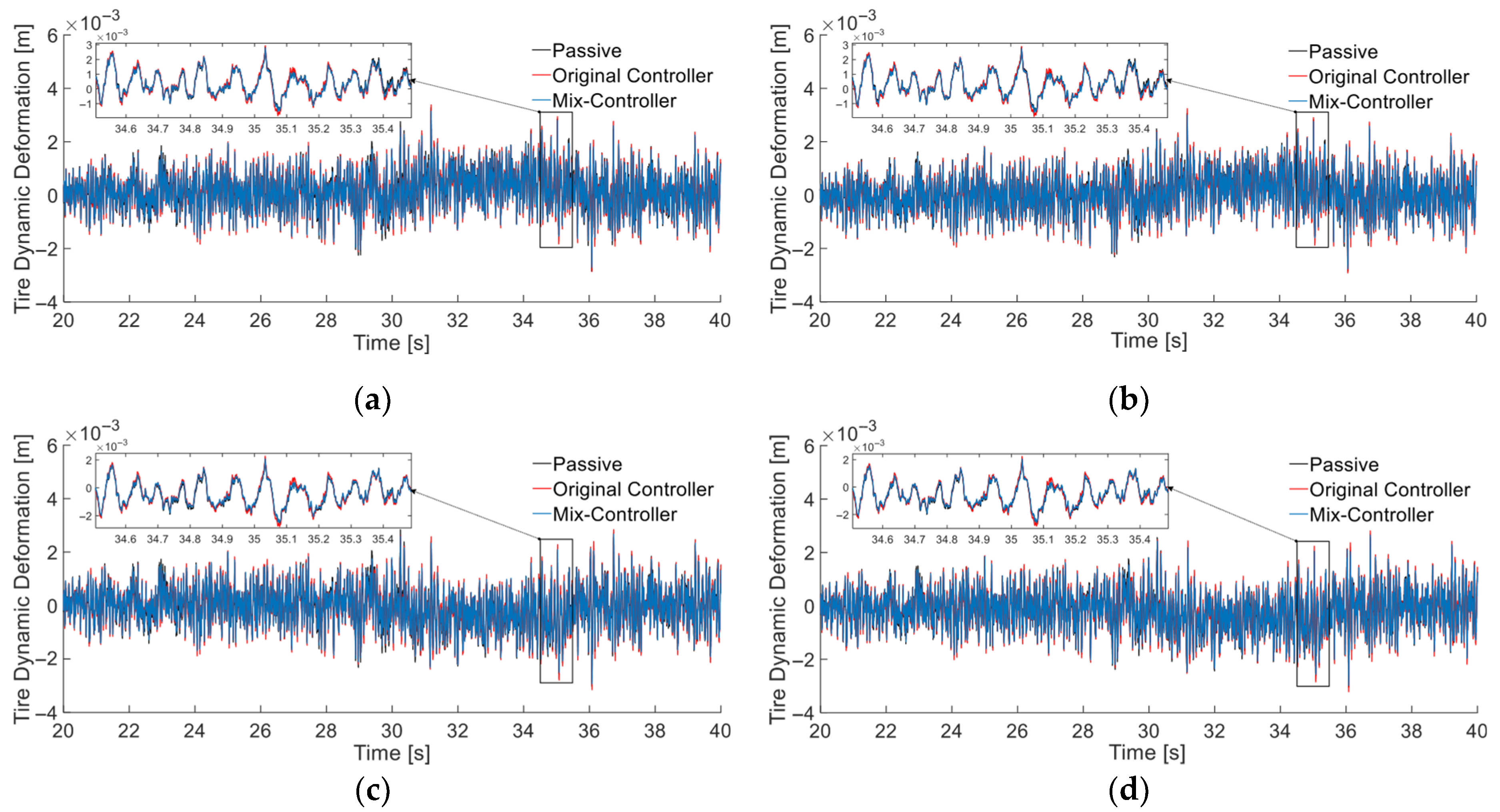
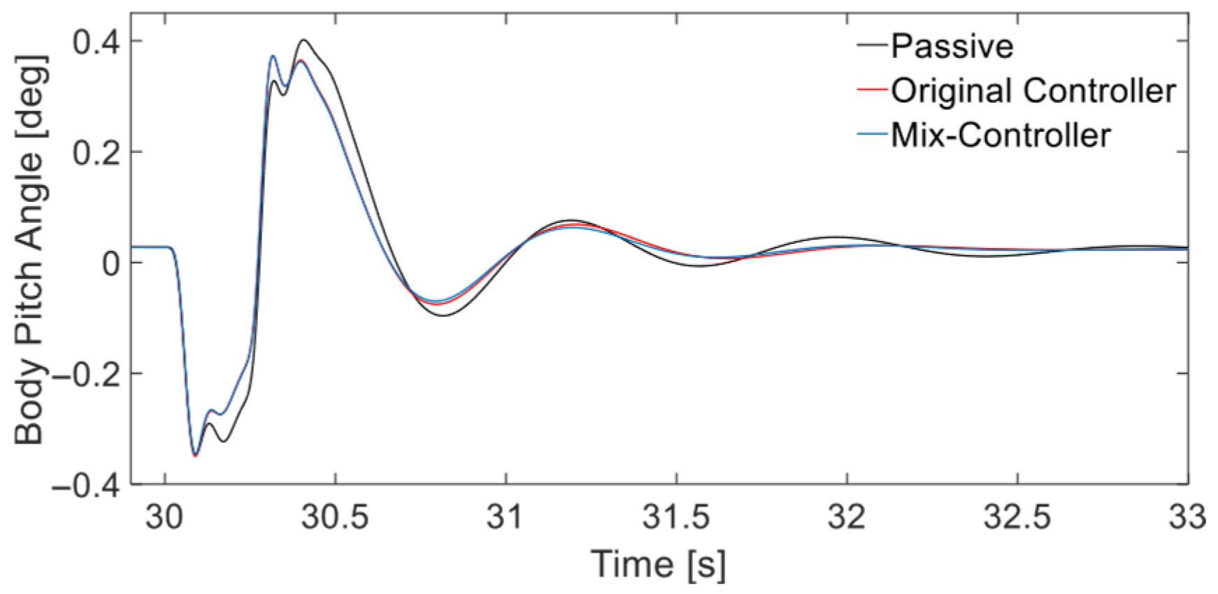
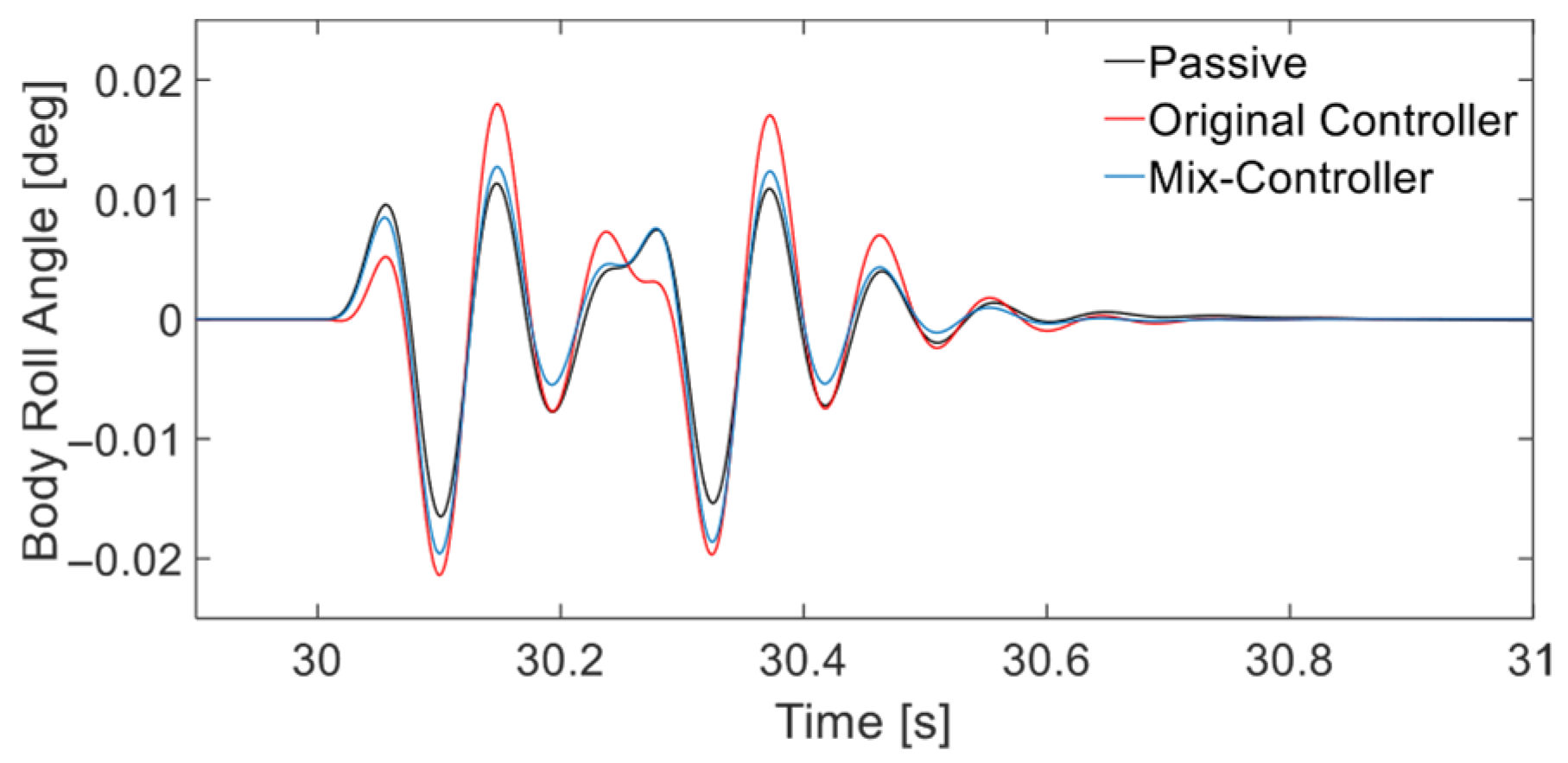
Time-Domain Response Analysis

Table 7. Root mean square plant for each evaluation metric.

		Passive	Original Controller	Rate of Change of Original Controller vs. Passive/%	Mix Controller	Rate of Change of Mix Controller vs. Passive/%
Body vertical acceleration (m·s−2)		0.16	0.13	18.33	0.15	7.95
Body roll angle (deg)		0.19	0.054	72.46	0.053	72.8
Body pitch angle (deg)		0.033	0.031	7.73	0.031	7.2
Suspension deflection (m)	Wheel 1	0.0034	0.0022	35.16	0.0021	38.23
	Wheel 2	0.0028	0.0019	33.28	0.0018	36.52
	Wheel 3	0.0031	0.0021	30.54	0.002	34.22
	Wheel 4	0.0032	0.0021	35.62	0.002	38.66
Tire dynamic deformation (m)	Wheel 1	0.00071	0.00072	−1.8	0.00068	3.76
	Wheel 2	0.00069	0.00071	−3.05	0.00067	2.72
	Wheel 3	0.00072	0.00074	−2.7	0.00069	3.58
	Wheel 4	0.00073	0.00075	−3.4	0.00071	2.62

Note $i=1,2,3,4$, are the left front wheel, left rear wheel, right front wheel, and right rear wheel, respectively.

shows the comparison of the root mean square (RMS) plant for each evaluation metric.

Figure 9, Figure 10 and Figure 11 show the time-domain response curves characterizing the body attitude control quantities on random road surface: body pitch angle, body roll angle, and suspension dynamic deflection.

Combined with Figure 9, Figure 10 and Figure 11 and Table 7, it can be seen that, compared with the passive suspension, the mix controller reduces the RMS root-plant of body roll angle and pitch angle by 72.80% and 7.20%, respectively, and the suspension dynamic deflection is reduced by an average of 36.91%. Compared with the original controller, the mix controller body roll angle and pitch angle maintain a similar RMS value, while the suspension dynamic deflection is reduced by an average of 3.26%, achieving better control of the vehicle body attitude.

Figure 12 and Figure 13 show the time-domain response curves characterizing the dynamic response to body vertical acceleration and tire dynamic deformation on random road surface.

As can be seen from Figure 12 and Figure 13, the mix controller reduces the body vertical acceleration and tire dynamic deformation compared to passive suspension. Combined with the comparison of the rms values in Table 3, compared to the passive suspension, the mix controller reduced the body vertical acceleration by 7.95% and the original controller reduced the body vertical acceleration by 18.33%; the mix controller reduced the tire dynamic deformation by an average of 3.17% and the original controller increased the tire dynamic deformation by an average of 2.74%. The result shows that the mix controller makes the tire dynamic deformation smaller.

The results show that the mix controller proposed in this paper, for the passive suspension, all the metrics are reduced; for the original controller, although the body vertical acceleration is deteriorated, the degree of deterioration is within the acceptable range, and when the vehicle mass is 2000 kg, safety is especially important. The control of the suspension dynamic deformation and tire dynamic deformation is more critical. If the original controller is used for vehicle control, it causes a deviation from the preset required control.

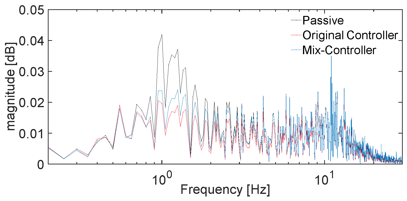
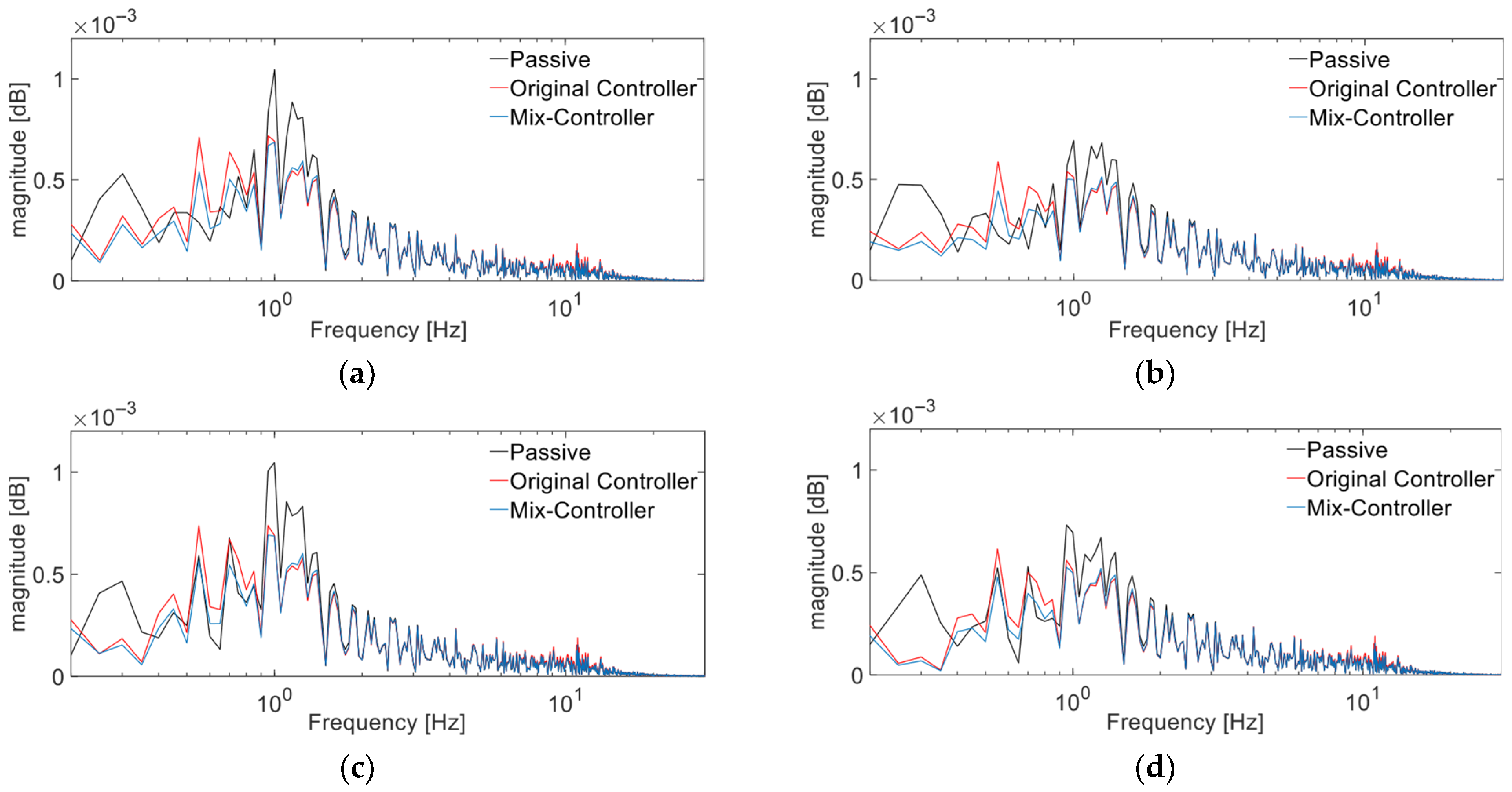
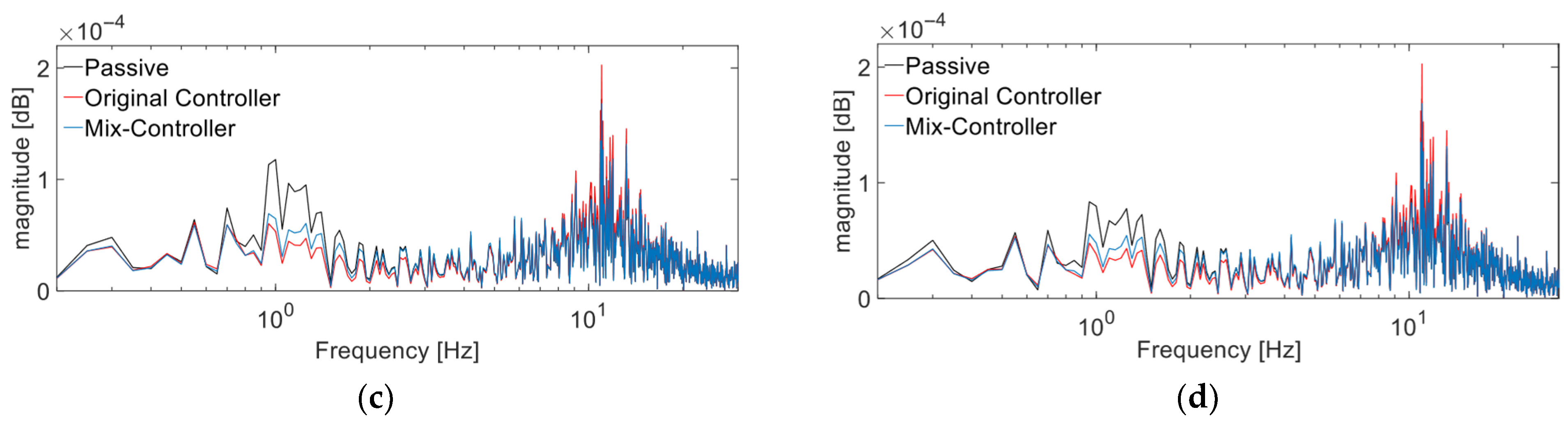
Frequency-Domain Response Analysis

The frequency-domain response curve of body vertical acceleration on random road surface is shown in Figure 14.

From the frequency-domain analysis in Figure 13, it can be seen that, compared with the passive suspension, the mix controller body vertical acceleration response has a significant reduction at the first-order resonance peak and little change at the second-order resonance peak; compared with the original controller, the mix controller body vertical acceleration response is slightly higher at the first-order resonance peak and at the second-order resonance peak, but it is still within a reasonable range.

The frequency-domain response curves of suspension dynamic deflection and tire dynamic deformation on random road surface are shown in Figure 15 and Figure 16.

From the frequency domain analysis in Figure 15, it can be seen that, compared with the passive suspension and the original controller, the mix controller suspension dynamic deflection response is reduced at both the first-order resonance peak and the second-order resonance peak. Among them, for the passive suspension, the mix controller suspension dynamic deflection response is significantly reduced at the first-order resonance peak, and for the original controller, the mix controller suspension dynamic deflection response is significantly reduced at the second-order resonance peak. The results show that the mix controller is more effective in the control of the suspension dynamic deflection.

From the frequency domain analysis in Figure 16, it can be seen that, compared with the passive suspension, both the original controller and the mix controller tire dynamic deformation responses are significantly reduced at the first-order resonance peaks, where the original controller is slightly better than the mix controller; at the second-order resonance peaks, the original controller tire dynamic deformation response is significantly higher compared with the passive suspension, whereas the mix controller tire dynamic deformation response does not change much compared with the passive suspension.

Comprehensive analysis of the above, in the case of the total mass of the truck, is 2 t; the comfort of the mix controller has a lower degree of deterioration, but greatly guarantees the safety performance of the vehicle in the case of heavy loads, and the results show that the mix controller has very good adaptability to the various cases of the truck mass.

5.3. Analysis of Actuator Force and Efficiency

Figure 17 shows a comparison of the actuator force for the original controller and the mix controller.

As shown in Figure 17a, the amplitude of the actuator force of the original controller is, in general, larger and less efficient than that of the mix controller. As shown in Figure 17b, the original controller causes a high frequency actuator force component to be output from the active suspension, whereas the mix controller’s high frequency component is greatly reduced, and such improvement reduces the requirement of the active suspension actuator response speed, which is beneficial to the design of the active suspension actuator. In conclusion, the mix controller not only makes the design of active suspension less complicated but also enables the utilization and performance of active suspension to be improved compared with the original controller.

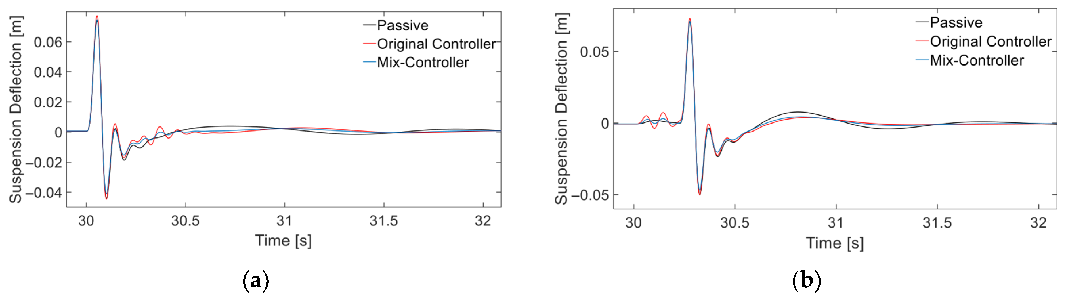
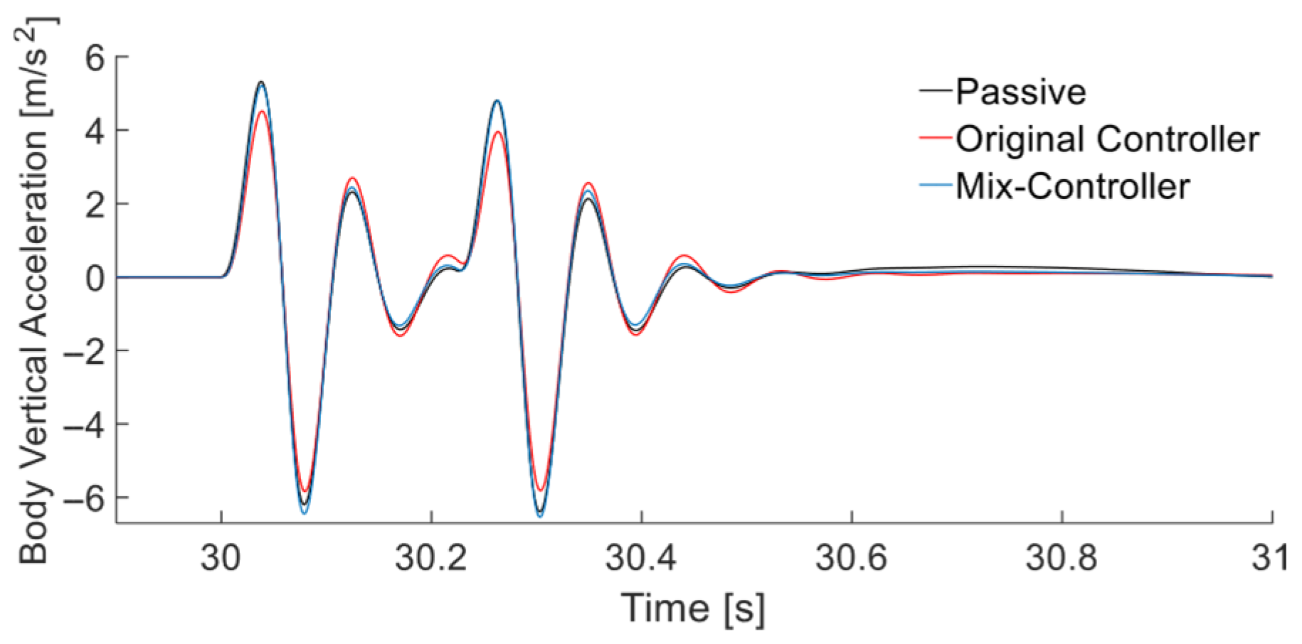
5.4. A Road Bump Experimentation Simulation Analysis

To analyze the effect of the mix controller more comprehensively, a road bump is set up at 30 s. In this simulation, the longitudinal acceleration is the same as above, and there is no lateral acceleration.

Figure 18, Figure 19 and Figure 20 show the time-domain response curves characterizing the body attitude control quantities on a road bump: body pitch angle, body roll angle, and suspension dynamic deflection.

Combined with Figure 18, Figure 19 and Figure 20, compared with the passive suspension, the maximum pitch angle of the mix controller has been significantly reduced, the maximum roll angle has been slightly increased, and the maximum suspension dynamic deflections have remained the same, and the mix controller has a shorter adjustment time for the body attitude control quantities. Compared with the original controller, the maximum pitch angle of the mix controller has remained, the maximum roll angle and maximum suspension dynamic deflection have been significantly reduced, and the mix controller has a shorter adjustment time for body attitude control quantities.

Figure 21 and Figure 22 show the time-domain response curves characterizing the dynamic response to body vertical acceleration and tire dynamic deformation on a road bump.

Combined with Figure 21 and Figure 22, compared to the passive suspension, the maximum body vertical acceleration and tire dynamic deformation of the mix controller have been slightly reduced, and the mix controller has a shorter adjustment time for its dynamic response. Compared to the original controller, the maximum body vertical acceleration of the mix controller has been increased, while the maximum dynamic deformation remains unchanged. Additionally, the mix controller has a shorter adjustment time for its dynamic response.

6. Conclusions

In this paper, research on active suspension has been carried out on trucks, and the main conclusions are as follows:

(1)

The mix controller for the active suspension of trucks integrated with online estimation of vehicle mass is proposed. Compared to the original controller, the mix controller can adapt to the real-time changes in vehicle mass and has a better control effect, ensuring the effectiveness of the control system.

(2)

According to the characteristics of parameter changes in the vehicle driving process, based on longitudinal vehicle dynamics using FFRLS and simulation test verification, the final mass estimation error results are less than 5%.

(3)

According to the simulation results, compared to the original controller, in the time domain, the suspension dynamic deflection and tire dynamic deformation of the mix controller are reduced by an average of 3.26% and 5.91%, respectively, in the frequency domain, the suspension dynamic deflection response and tire dynamic deformation induced by external excitation of the mix controller are generally better than those of the original controller. On the other hand, although some metrics have deteriorated in the time and frequency domains, overall global optimization of comfort and stability in attitude can still be achieved.

References

1. Theunissen, J.; Tota, A.; Gruber, P.; Dhaens, M.; Sorniotti, A. Preview-based Techniques for Vehicle Suspension Control: A State-of-the-art Review. Annu. Rev. Control 2021, 51, 206–235. [Google Scholar] [CrossRef]
2. Kimball, J.B.; DeBoer, B.; Bubbar, K. Adaptive Control and Reinforcement Learning for Vehicle Suspension Control: A review. Annu. Rev. Control. 2024, 58, 100974. [Google Scholar] [CrossRef]
3. Yu, M.; Evangelou, S.A.; Dini, D. Advances in Vehicle Suspension Systems. Engineering 2024, 33, 160–177. [Google Scholar] [CrossRef]
4. Hassan, M.A.; Abdelkareem, M.A.A.; Moheyeldein, M.M.; Elagouz, A.; Tan, G. Advanced Study of Tire Characteristics and Their Influence on Vehicle Lateral Stability and Untripped Rollover Threshold. Alex. Eng. J. 2020, 59, 1613–1628. [Google Scholar] [CrossRef]
5. Wei, W.; Yu, S.J.; Li, B.Z. Research on Magnetic Characteristics and Fuzzy PID Control of Electromagnetic Suspension. Actuators 2023, 12, 203. [Google Scholar] [CrossRef]
6. Liu, L.; Ren, Y.-J.; Shen, T.; Yin, G.-T.; Zhang, Y.-J. Grade Recognition for Electric Vehicles with Vehicle Mass Estimation. J. Jilin Univ. (Eng. Technol. Ed.) 2025, 55, 846–856. [Google Scholar] [CrossRef]
7. Peng, C.; Wei, C.; Solernou, A.; Hagenzieker, M.; Merat, N. User Comfort and Naturalness of Automated Driving: The Effect of Vehicle Kinematic and Proxemic Factors on Subjective Response. Appl. Ergon. 2025, 122, 104397. [Google Scholar] [CrossRef]
8. Zheng, W.G.; Zhang, J.-Z.; Wang, S.-C.; Feng, G.-S.; Xu, X.-H.; Ma, Q.X. A Shifting Strategy for Electric Commercial Vehicles Considering Mass and Gradient Estimation. Cmes-Comput. Model. Eng. Sci. 2023, 137, 489–508. [Google Scholar] [CrossRef]
9. Yang, M.; Tian, J. Longitudinal and Lateral Stability Control Strategies for ACC Systems of Differential Steering Electric Vehicles. Electronics 2023, 12, 4178. [Google Scholar] [CrossRef]
10. Liao, Y.S.; Hu, Z.-M.; Jia, H.-B.; Tian, Y.-C.; Zhong, S.-H.; Peng, X.-L. Vehicle Mass and Road Grade Estimation Based on Longitudinal-Lateral Dynamics Coupling. Automot. Eng. 2024, 1–7. [Google Scholar] [CrossRef]
11. Gao, L.; Wu, Q.; He, Y. Road slope estimation for heavy-duty vehicles under the influence of multiple source factors in real complex road environments. Mech. Syst. Signal Process. 2024, 208, 110973. [Google Scholar] [CrossRef]
12. Shangguan, J.Y.; Yue, M.; Xu, C.; Zhao, J. Robust Fault-Tolerant Estimation of Sideslip and Roll Angles for Distributed Drive Electric Buses with Stochastic Passenger Mass. IEEE Trans. Intell. Transp. Syst. 2023, 24, 14480–14489. [Google Scholar] [CrossRef]
13. Smith, J.; Johnson, A. The Impact of Suspension System Tuning on Vehicle Handling and Ride Comfort. J. Automot. Eng. 2023, 305, 567–580. [Google Scholar]
14. Liu, C.N.; Chen, L.; Lee, H.P.; Yang, Y.; Zhang, X.L. Generalized Skyhook-Groundhook Hybrid Strategy and Control on Vehicle Suspension. IEEE Trans. Veh. Technol. 2023, 72, 1689–1700. [Google Scholar] [CrossRef]
15. Hussan, U.; Majeed, M.A.; Asghar, F.; Waleed, A.; Khan, A.; Javed, M.R. Fuzzy logic-based voltage regulation of hybrid energy storage system in hybrid electric vehicles. Electr. Eng. 2022, 104, 485–495. [Google Scholar] [CrossRef]
16. Jovanovic, A.; Teodorovic, D. Type-2 fuzzy logic based transit priority strategy. Expert Syst. Appl. 2022, 187, 115875. [Google Scholar] [CrossRef]
17. Li, H.; Yang, X. Robust optimal control of logical control networks with function perturbation. Automatica 2023, 152, 110970. [Google Scholar] [CrossRef]
18. Mai, H.; Chen, X.; Yin, Z. Time-optimal L1/L2 norms optimal control for linear time-invariant systems. Optim. Control. Appl. Methods 2023, 44, 1686–1699. [Google Scholar] [CrossRef]
19. Han, M.; Li, Z.; Yin, X.; Yin, X. Robust Learning and Control of Time-Delay Nonlinear Systems with Deep Recurrent Koopman Operators. IEEE Trans. Ind. Inform. 2024, 20, 4675–4684. [Google Scholar] [CrossRef]
20. Kumar, L.; Kumar, P.; Dhillon, S.S. A Multiobjective Optimization Approach for Linear Quadratic Gaussian/Loop Transfer Recovery Design. Optim. Control. Appl. Methods 2020, 41, 1267–1287. [Google Scholar] [CrossRef]
21. Kader, A.M.; El-Gamal, H.A.; Abdelnaeem, M. Influence of Pneumatic Tire Enveloping Behavior Characteristics on the Performance of a Half Car Suspension System Using Multi-Objective Optimization Algorithms. Alex. Eng. J. 2024, 107, 298–316. [Google Scholar] [CrossRef]
22. Nan, Y.; Shao, S.J.; Ren, C.B.; Wu, K.W.; Cheng, Y.J.; Zhou, P.C. Simulation and Experimental Research on Active Suspension System with Time-Delay Feedback Control. IEEE Access 2023, 11, 88498–88510. [Google Scholar] [CrossRef]
23. Wang, M.Q.; Zeng, S.H.; He, Y.X.; Su, S.; Liu, P.F. Multi-Objective Optimization of a Fractional-Order Control System for an EMS-Type Maglev Model. IEEE Trans. Veh. Technol. 2024, 73, 12652–12667. [Google Scholar] [CrossRef]
24. He, L.Q.; Pan, Y.J.; He, Y.S.; Li, Z.X.; Królczyk, G.; Du, H.P. Control Strategy for Vibration Suppression of a Vehicle Multibody System on a Bumpy Road. Mech. Mach. Theory 2022, 174, 104891. [Google Scholar] [CrossRef]
25. Mastinu, G.; Della Rossa, F.; Previati, G.; Gobbi, M.; Fainello, M. Global stability of road vehicle motion with driver control. Nonlinear Dyn. 2023, 111, 18043–18059. [Google Scholar] [CrossRef]
26. Rong, J.L.; Deng, Z.K.; He, L.; Wang, X.; Cheng, X.Y. Time-Domain Simulation and Optimization of Ride Comfort for Vehicle Active Suspension. Trans. Beijing Inst. Technol. 2022, 42, 46–52. [Google Scholar] [CrossRef]
27. Duc Ngoc, N.; Tuan Anh, N. Evaluate the stability of the vehicle when using the active suspension system with a hydraulic actuator controlled by the OSMC algorithm. Sci. Rep. 2022, 12, 19364. [Google Scholar] [CrossRef]
28. Nguyen, D.N.; Nguyen, T.A. Proposing an original control algorithm for the active suspension system to improve vehicle vibration: Adaptive fuzzy sliding mode proportional-integral-derivative tuned by the fuzzy (AFSPIDF). Heliyon 2023, 9, e14210. [Google Scholar] [CrossRef]
29. Viadero-Monasterio, F.; Boada, B.L.; Boada, M.J.L.; Diaz, V. H∞ dynamic output feedback control for a networked control active suspension system under actuator faults. Mech. Syst. Signal Process. 2022, 162, 10850. [Google Scholar] [CrossRef]
30. Zhang, J.H.; Ding, F.; Liu, J.; Lei, F.; Wang, Y.F.; Wei, C.F. Event Triggered Finite-Time Adaptive Sliding-Mode Coordinated Control of Uncertain Hysteretic Leaf Spring Suspension with Prescribed Performance. IEEE Trans. Intell. Transp. Syst. 2025, 26, 2621–2632. [Google Scholar] [CrossRef]
31. Paleologu, C.; Benesty, J.; Ciochina, S. Data-Reuse Recursive Least-Squares Algorithms. IEEE Signal Process. Lett. 2022, 29, 752–756. [Google Scholar] [CrossRef]
32. Han, Z.; Zhang, F.; Zhang, Y.; Han, Y.; Jiang, P. Improved Variable Forgetting Factor Proportionate RLS Algorithm with Sparse Penalty and Fast Implementation Using DCD Iterations. China Commun. 2024, 21, 16–27. [Google Scholar] [CrossRef]
33. Wu, G.Y.; Rui, X.T.; Wang, G.P.; Jiang, M.; Wang, X. Modelling and simulation of driving dynamics of wheeled launch system under random road surface excitation. Acta Mech. Sin. 2024, 40, 523310. [Google Scholar] [CrossRef]
34. Xing, C.; Zhu, Y.; Wu, H. Electromechanical Coupling Braking Control Strategy Considering Vertical Vibration Suppression for Vehicles Driven by In-Wheel Motors. IEEE-Asme Trans. Mechatron. 2022, 27, 5701–5711. [Google Scholar] [CrossRef]
Figure 1. Multi-degree-of-freedom coupling dynamics model.
Vehicles 07 00071 g001
Figure 2. Architecture for LQR Controller.
Vehicles 07 00071 g002
Figure 3. Architecture for Mix Controller.
Vehicles 07 00071 g003
Figure 4. Vehicle longitudinal speed.
Vehicles 07 00071 g004
Figure 5. Vehicle longitudinal acceleration.
Vehicles 07 00071 g005
Figure 6. Vehicle mass estimation result.
Vehicles 07 00071 g006
Figure 7. Mean-processed mass estimation result.
Vehicles 07 00071 g007
Figure 8. Vehicle lateral and longitudinal acceleration.
Vehicles 07 00071 g008
Figure 9. Time-domain response curve of body pitch angle on random road surface.
Vehicles 07 00071 g009
Figure 10. Time-domain response curve of body roll angle on random road surface.
Vehicles 07 00071 g010
Figure 11. Time-domain response curve of suspension dynamic deflection on random road surface: (a) Wheel 1; (b) Wheel 2; (c) Wheel 3; (d) Wheel 4.
Vehicles 07 00071 g011
Figure 12. Time-domain response curve of body vertical acceleration on random road surface.
Vehicles 07 00071 g012
Figure 13. Time-domain response curve of tire dynamic deformation on random road surface: (a) Wheel 1; (b) Wheel 2; (c) Wheel 3; (d) Wheel 4.
Vehicles 07 00071 g013
Figure 14. Frequency-domain response curve of body vertical acceleration on random road surface.
Vehicles 07 00071 g014
Figure 15. Frequency-domain response curve of suspension dynamic deflection on random road surface: (a) Wheel 1; (b) Wheel 2; (c) Wheel 3; (d) Wheel 4.
Vehicles 07 00071 g015
Figure 16. Frequency-domain response curve of tire dynamic deformation on random road surface: (a) Wheel 1; (b) Wheel 2; (c) Wheel 3; (d) Wheel 4.
Vehicles 07 00071 g016aVehicles 07 00071 g016b
Figure 17. Comparison of actuator force: (a) Time-domain comparison; (b) Frequency-domain comparison.
Vehicles 07 00071 g017
Figure 18. Time-domain response curve of body pitch angle on a road bump.
Vehicles 07 00071 g018
Figure 19. Time-domain response curve of body roll angle on a road bump.
Vehicles 07 00071 g019
Figure 20. Time-domain response curve of suspension dynamic deflection on a road bump: (a) Wheel 1; (b) Wheel 2.
Vehicles 07 00071 g020
Figure 21. Time-domain response curve of body vertical acceleration on a road bump.
Vehicles 07 00071 g021
Figure 22. Time-domain response curve of tire dynamic deformation on a road bump: (a) Wheel 1; (b) Wheel 2.
Vehicles 07 00071 g022